
SNPtotree—Resolving the Phylogeny of SNPs on Non-Recombining DNA

Abstract
:1. Introduction
2. Materials and Methods
2.1. SNPtotree
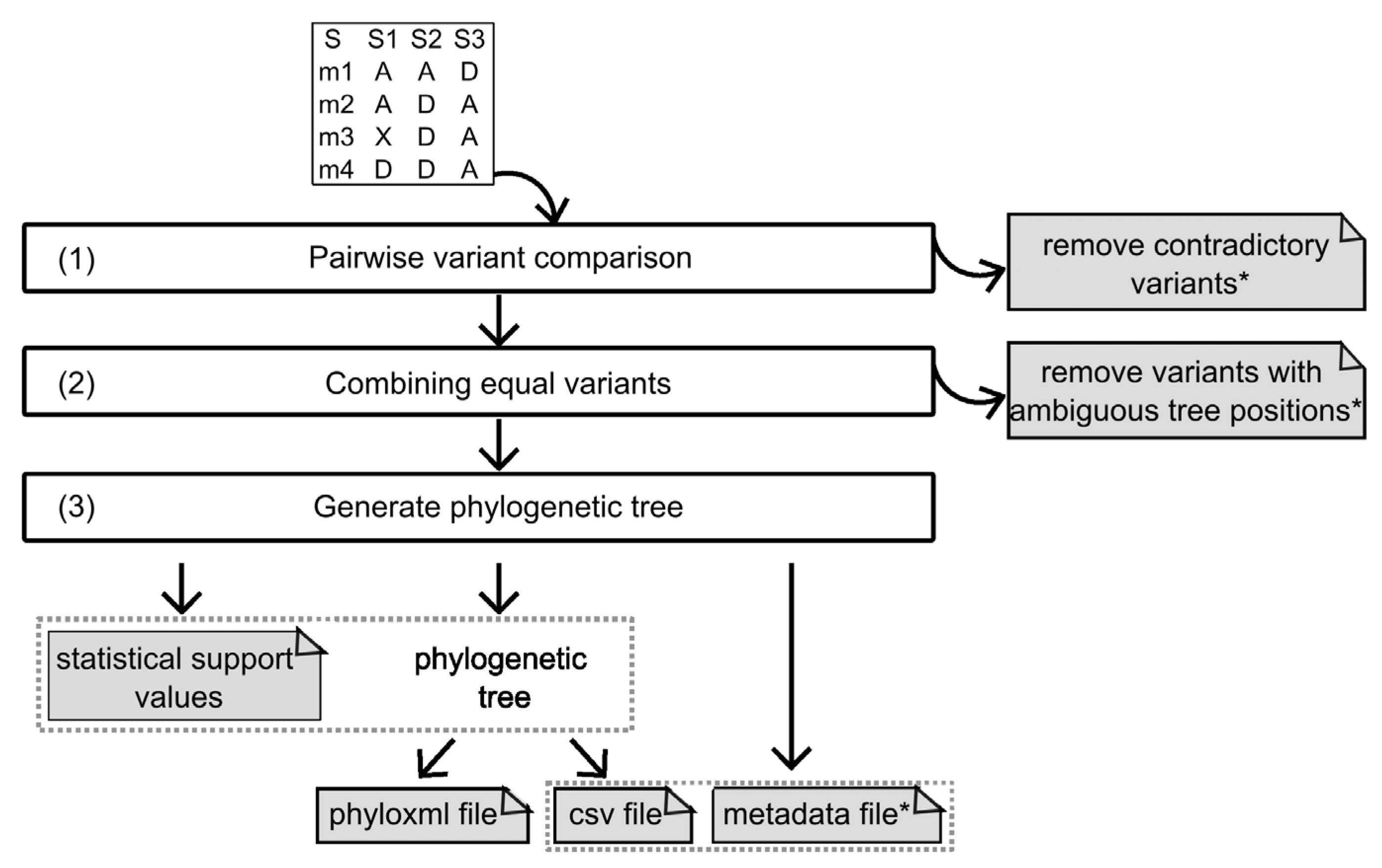
2.1.1. Input
2.1.2. Output Files
2.1.3. Algorithm
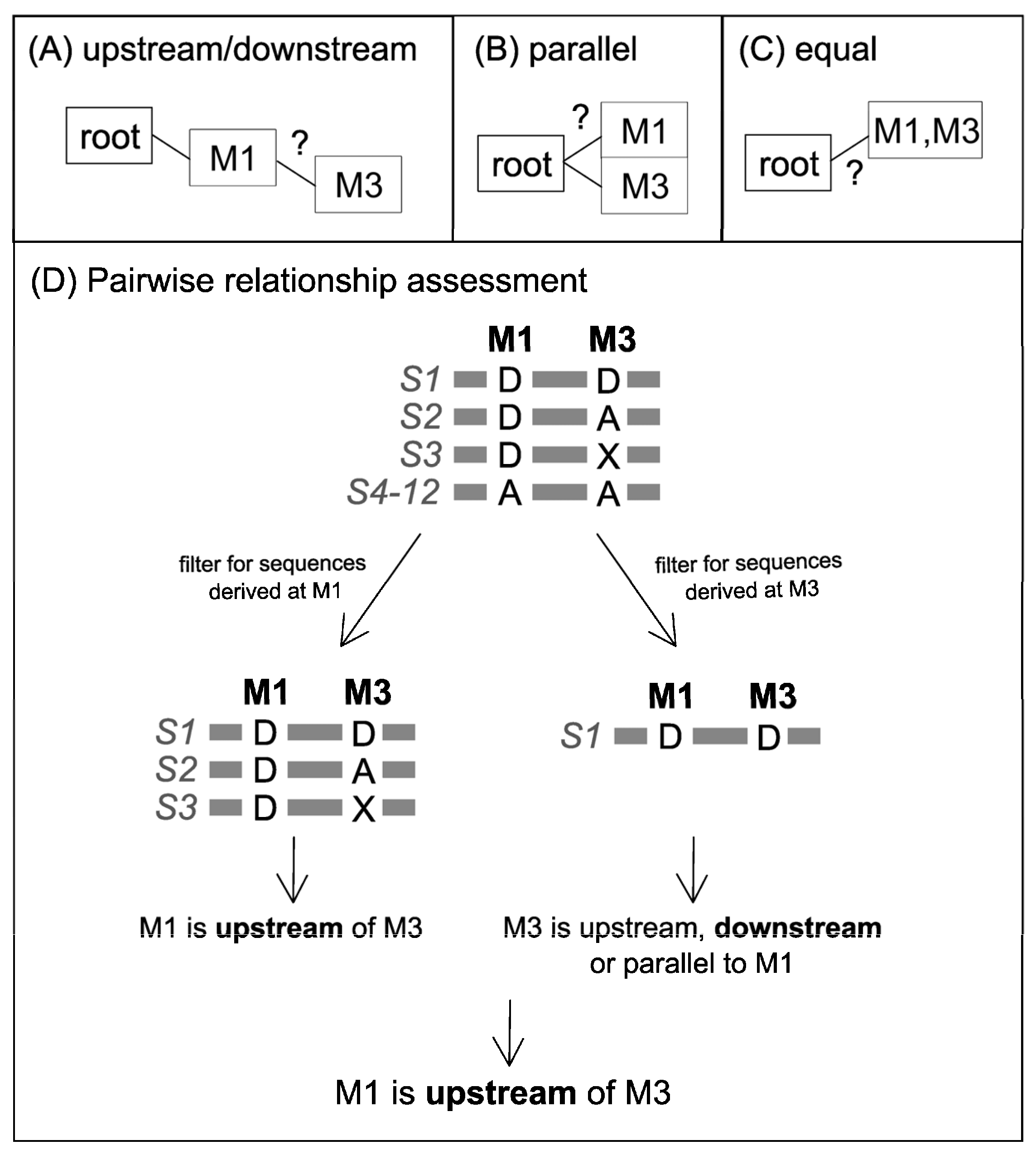
Pairwise Variant Comparison and Removal of Variants with Contradictory Predictions
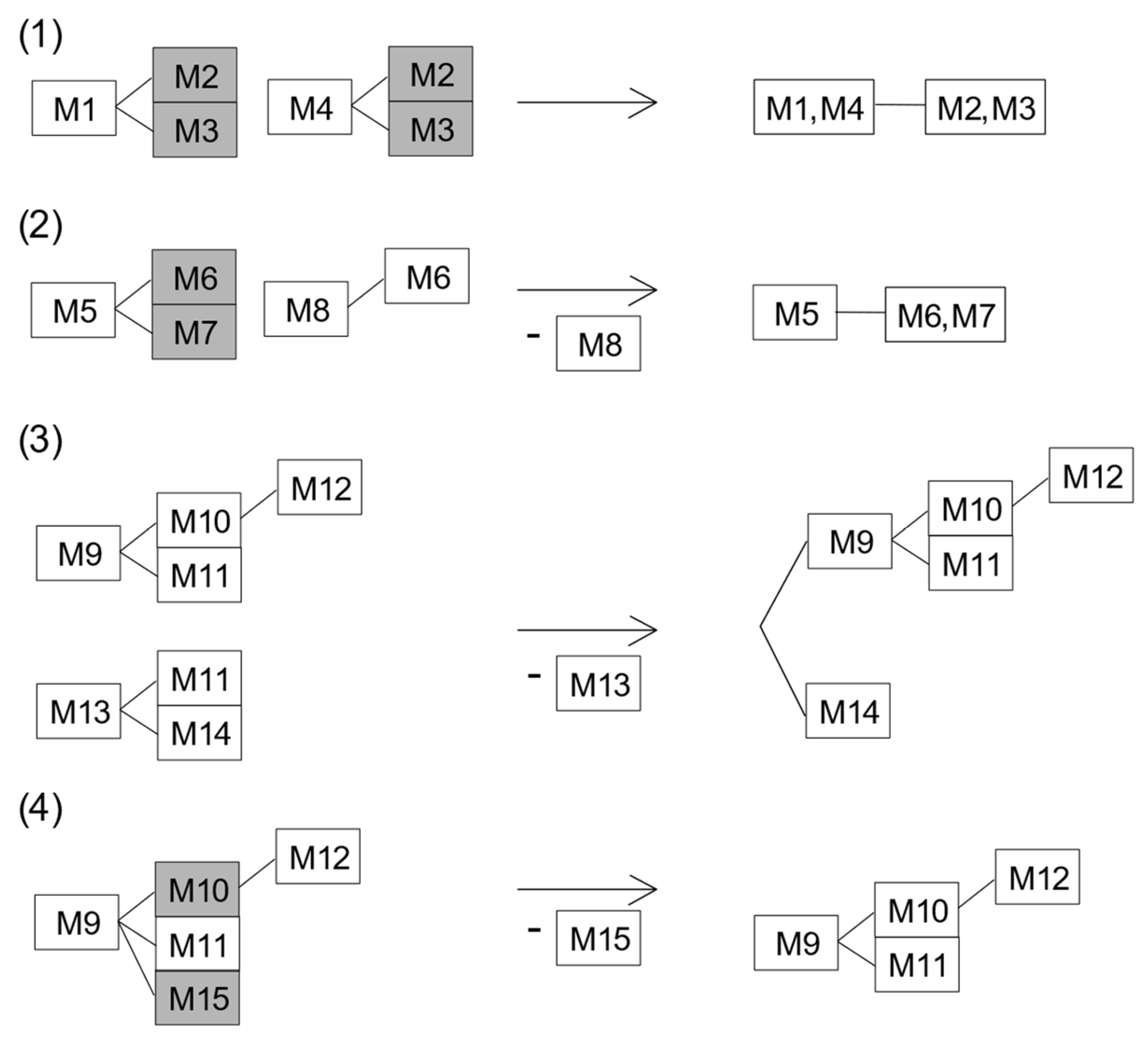
Combining Equal Variants and the Removal of Variants with Ambiguous Results
Generating the Phylogenetic Tree
2.2. Datasets and Nomenclature
2.3. Maximum Likelihood Phylogenetic Trees Using RAxML
3. Results and Discussion
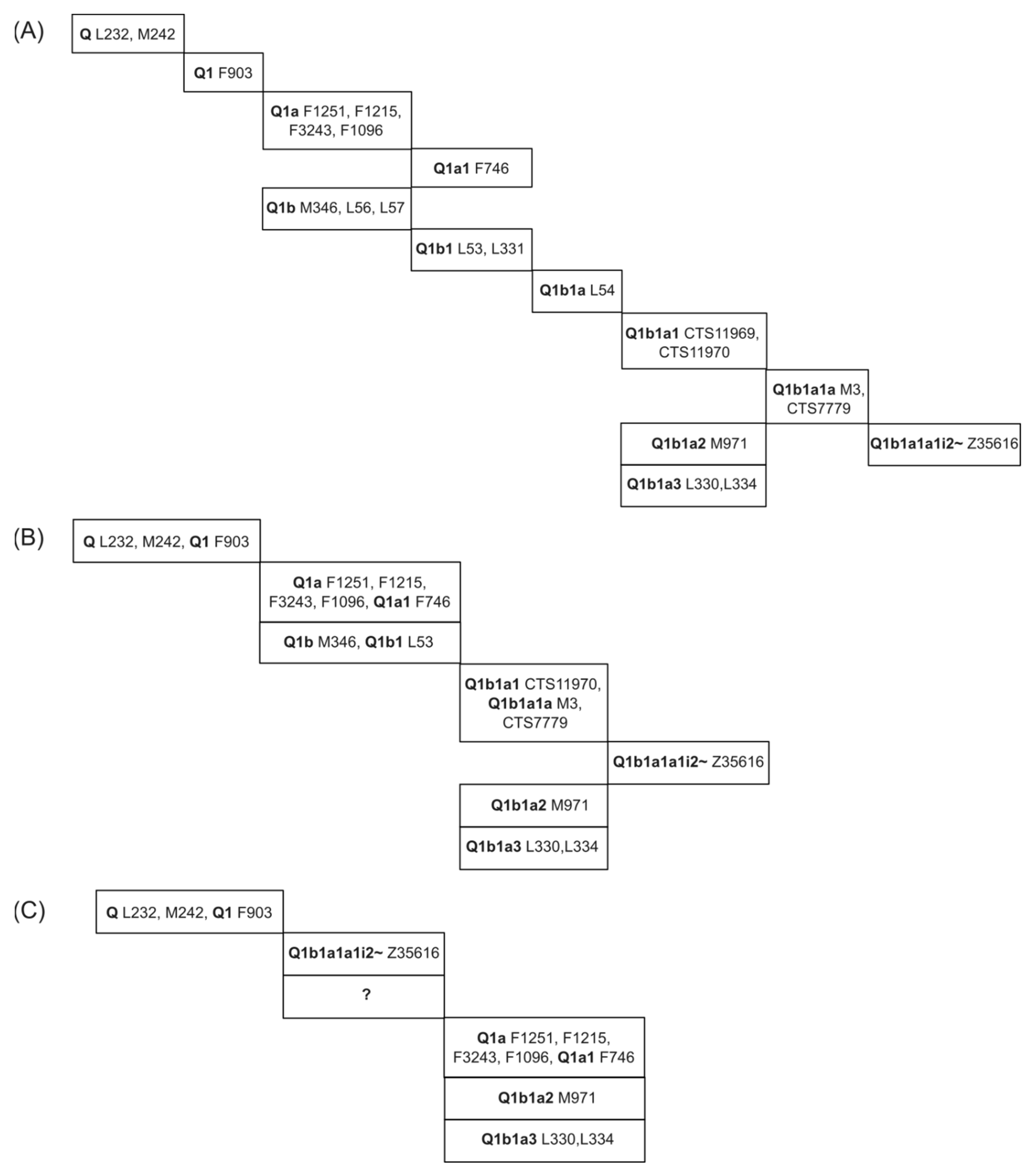
3.1. Comparing SNP Phylogeny Trees of Testdata 1 by Using SNPtotree and Maximum Likelihood (ML) Trees
3.2. Exploring the Correlation and Extent of Missing Data and Tree Resolution Using the Comprehensive Testdata 2
4. Conclusions
Supplementary Materials
Author Contributions
Funding
Institutional Review Board Statement
Informed Consent Statement
Data Availability Statement
Conflicts of Interest
References
- Ishikawa, S.A.; Zhukova, A.; Iwasaki, W.; Gascuel, O. A Fast Likelihood Method to Reconstruct and Visualize Ancestral Scenarios. Mol. Biol. Evol. 2019, 36, 2069–2085. [Google Scholar] [CrossRef] [PubMed]
- Joy, J.B.; Liang, R.H.; McCloskey, R.M.; Nguyen, T.; Poon, A.F.Y. Ancestral Reconstruction. PLoS Comput. Biol. 2016, 12, e1004763. [Google Scholar] [CrossRef] [PubMed]
- Guyeux, C.; Al-Nuaimi, B.; AlKindy, B.; Couchot, J.-F.; Salomon, M. On the Reconstruction of the Ancestral Bacterial Genomes in Genus Mycobacterium and Brucella. BMC Syst. Biol. 2018, 12, 100. [Google Scholar] [CrossRef] [PubMed]
- Lemey, P.; Rambaut, A.; Drummond, A.J.; Suchard, M.A. Bayesian Phylogeography Finds Its Roots. PLoS Comput. Biol. 2009, 5, e1000520. [Google Scholar] [CrossRef] [PubMed]
- King, T.E.; Jobling, M.A. What’s in a Name? Y Chromosomes, Surnames and the Genetic Genealogy Revolution. Trends Genet. 2009, 25, 351–360. [Google Scholar] [CrossRef] [PubMed]
- Mizuno, N.; Kitayama, T.; Fujii, K.; Nakahara, H.; Yoshida, K.; Sekiguchi, K.; Yonezawa, N.; Nakano, M.; Kasai, K. A Forensic Method for the Simultaneous Analysis of Biallelic Markers Identifying Y Chromosome Haplogroups Inferred as Having Originated in Asia and the Japanese Archipelago. Forensic Sci. Int. Genet. 2010, 4, 73–79. [Google Scholar] [CrossRef] [PubMed]
- Chiaroni, J.; Underhill, P.A.; Cavalli-Sforza, L.L. Y Chromosome Diversity, Human Expansion, Drift, and Cultural Evolution. Proc. Natl. Acad. Sci. USA 2009, 106, 20174–20179. [Google Scholar] [CrossRef]
- Underhill, P.A.; Kivisild, T. Use of y Chromosome and Mitochondrial DNA Population Structure in Tracing Human Migrations. Annu. Rev. Genet. 2007, 41, 539–564. [Google Scholar] [CrossRef]
- Felsenstein, J. Evolutionary Trees from DNA Sequences: A Maximum Likelihood Approach. J. Mol. Evol. 1981, 17, 368–376. [Google Scholar] [CrossRef]
- Stamatakis, A. RAxML Version 8: A Tool for Phylogenetic Analysis and Post-Analysis of Large Phylogenies. Bioinformatics 2014, 30, 1312–1313. [Google Scholar] [CrossRef]
- Nguyen, L.-T.; Schmidt, H.A.; von Haeseler, A.; Minh, B.Q. IQ-TREE: A Fast and Effective Stochastic Algorithm for Estimating Maximum-Likelihood Phylogenies. Mol. Biol. Evol. 2015, 32, 268–274. [Google Scholar] [CrossRef] [PubMed]
- Guindon, S.; Dufayard, J.-F.; Lefort, V.; Anisimova, M.; Hordijk, W.; Gascuel, O. New Algorithms and Methods to Estimate Maximum-Likelihood Phylogenies: Assessing the Performance of PhyML 3.0. Syst. Biol. 2010, 59, 307–321. [Google Scholar] [CrossRef] [PubMed]
- Tamura, K.; Stecher, G.; Kumar, S. MEGA11: Molecular Evolutionary Genetics Analysis Version 11. Mol. Biol. Evol. 2021, 38, 3022–3027. [Google Scholar] [CrossRef] [PubMed]
- Zou, Z.; Zhang, H.; Guan, Y.; Zhang, J. Deep Residual Neural Networks Resolve Quartet Molecular Phylogenies. Mol. Biol. Evol. 2020, 37, 1495–1507. [Google Scholar] [CrossRef] [PubMed]
- Suvorov, A.; Hochuli, J.; Schrider, D.R. Accurate Inference of Tree Topologies from Multiple Sequence Alignments Using Deep Learning. Syst. Biol. 2020, 69, 221–233. [Google Scholar] [CrossRef] [PubMed]
- Leuchtenberger, A.F.; Crotty, S.M.; Drucks, T.; Schmidt, H.A.; Burgstaller-Muehlbacher, S.; von Haeseler, A. Distinguishing Felsenstein Zone from Farris Zone Using Neural Networks. Mol. Biol. Evol. 2020, 37, 3632–3641. [Google Scholar] [CrossRef] [PubMed]
- Bouckaert, R.; Vaughan, T.G.; Barido-Sottani, J.; Duchêne, S.; Fourment, M.; Gavryushkina, A.; Heled, J.; Jones, G.; Kühnert, D.; Maio, N.D.; et al. BEAST 2.5: An Advanced Software Platform for Bayesian Evolutionary Analysis. PLoS Comput. Biol. 2019, 15, e1006650. [Google Scholar] [CrossRef]
- Huelsenbeck, J.P.; Ronquist, F. MRBAYES: Bayesian Inference of Phylogenetic Trees. Bioinformatics 2001, 17, 754–755. [Google Scholar] [CrossRef]
- Bocakova, M.; Bocak, L.; Gimmel, M.L.; Motyka, M.; Vogler, A.P. Aposematism and Mimicry in Soft-Bodied Beetles of the Superfamily Cleroidea (Insecta). Zool. Scr. 2016, 45, 9–21. [Google Scholar] [CrossRef]
- Doorenweerd, C.; van Nieukerken, E.J.; Menken, S.B.J. A Global Phylogeny of Leafmining Ectoedemia Moths (Lepidoptera: Nepticulidae): Exploring Host Plant Family Shifts and Allopatry as Drivers of Speciation. PLoS ONE 2015, 10, e0119586. [Google Scholar] [CrossRef]
- Olanj, N.; Garnatje, T.; Sonboli, A.; Vallès, J.; Garcia, S. The Striking and Unexpected Cytogenetic Diversity of Genus Tanacetum L. (Asteraceae): A Cytometric and Fluorescent in Situ Hybridisation Study of Iranian Taxa. BMC Plant Biol. 2015, 15, 174. [Google Scholar] [CrossRef] [PubMed]
- Wiens, J.J.; Morrill, M.C. Missing Data in Phylogenetic Analysis: Reconciling Results from Simulations and Empirical Data. Syst. Biol. 2011, 60, 719–731. [Google Scholar] [CrossRef] [PubMed]
- Dunn, K.A.; McEachran, J.D.; Honeycutt, R.L. Molecular Phylogenetics of Myliobatiform Fishes (Chondrichthyes: Myliobatiformes), with Comments on the Effects of Missing Data on Parsimony and Likelihood. Mol. Phylogenet Evol. 2003, 27, 259–270. [Google Scholar] [CrossRef] [PubMed]
- Hartmann, S.; Vision, T.J. Using ESTs for Phylogenomics: Can One Accurately Infer a Phylogenetic Tree from a Gappy Alignment? BMC Evol. Biol. 2008, 8, 95. [Google Scholar] [CrossRef] [PubMed]
- Wiens, J.J. Missing Data and the Design of Phylogenetic Analyses. J. Biomed. Inform. 2006, 39, 34–42. [Google Scholar] [CrossRef] [PubMed]
- Darriba, D.; Weiß, M.; Stamatakis, A. Prediction of Missing Sequences and Branch Lengths in Phylogenomic Data. Bioinformatics 2016, 32, 1331–1337. [Google Scholar] [CrossRef] [PubMed]
- Pinheiro, D.; Santander-Jimenéz, S.; Ilic, A. PhyloMissForest: A Random Forest Framework to Construct Phylogenetic Trees with Missing Data. BMC Genom. 2022, 23, 377. [Google Scholar] [CrossRef] [PubMed]
- Yasui, N.; Vogiatzis, C.; Yoshida, R.; Fukumizu, K. imPhy: Imputing Phylogenetic Trees with Missing Information Using Mathematical Programming. IEEE/ACM Trans. Comput. Biol. Bioinform. 2020, 17, 1222–1230. [Google Scholar] [CrossRef]
- Howie, B.N.; Donnelly, P.; Marchini, J. A Flexible and Accurate Genotype Imputation Method for the Next Generation of Genome-Wide Association Studies. PLoS Genet. 2009, 5, e1000529. [Google Scholar] [CrossRef]
- Marchini, J.; Howie, B. Genotype Imputation for Genome-Wide Association Studies. Nat. Rev. Genet. 2010, 11, 499–511. [Google Scholar] [CrossRef]
- Marchini, J.; Howie, B.; Myers, S.; McVean, G.; Donnelly, P. A New Multipoint Method for Genome-Wide Association Studies by Imputation of Genotypes. Nat. Genet. 2007, 39, 906–913. [Google Scholar] [CrossRef] [PubMed]
- Browning, B.L.; Zhou, Y.; Browning, S.R. A One-Penny Imputed Genome from Next-Generation Reference Panels. Am. J. Hum. Genet. 2018, 103, 338–348. [Google Scholar] [CrossRef] [PubMed]
- Jobin, M.; Schurz, H.; Henn, B.M. IMPUTOR: Phylogenetically Aware Software for Imputation of Errors in Next-Generation Sequencing. Genome Biol. Evol. 2018, 10, 1248–1254. [Google Scholar] [CrossRef] [PubMed]
- Regueiro, M.; Cadenas, A.M.; Gayden, T.; Underhill, P.A.; Herrera, R.J. Iran: Tricontinental Nexus for Y-Chromosome Driven Migration. Hum. Hered. 2006, 61, 132–143. [Google Scholar] [CrossRef] [PubMed]
- Batini, C.; Ferri, G.; Destro-Bisol, G.; Brisighelli, F.; Luiselli, D.; Sánchez-Diz, P.; Rocha, J.; Simonson, T.; Brehm, A.; Montano, V.; et al. Signatures of the Preagricultural Peopling Processes in Sub-Saharan Africa as Revealed by the Phylogeography of Early Y Chromosome Lineages. Mol. Biol. Evol. 2011, 28, 2603–2613. [Google Scholar] [CrossRef]
- Karmin, M.; Saag, L.; Vicente, M.; Sayres, M.A.W.; Järve, M.; Talas, U.G.; Rootsi, S.; Ilumäe, A.-M.; Mägi, R.; Mitt, M.; et al. A Recent Bottleneck of Y Chromosome Diversity Coincides with a Global Change in Culture. Genome Res. 2015, 25, 459–466. [Google Scholar] [CrossRef] [PubMed]
- Kling, D.; Phillips, C.; Kennett, D.; Tillmar, A. Investigative Genetic Genealogy: Current Methods, Knowledge and Practice. Forensic Sci. Int. Genet. 2021, 52, 102474. [Google Scholar] [CrossRef]
- Parson, W.; Dür, A. EMPOP—A Forensic mtDNA Database. Forensic Sci. Int. Genet. 2007, 1, 88–92. [Google Scholar] [CrossRef]
- Willuweit, S.; Roewer, L. The New Y Chromosome Haplotype Reference Database. Forensic Sci. Int. Genet. 2015, 15, 43–48. [Google Scholar] [CrossRef]
- Gauthier, J.A.; Kearney, M.; Maisano, J.A.; Rieppel, O.; Behlke, A.D.B. Assembling the Squamate Tree of Life: Perspectives from the Phenotype and the Fossil Record. Bull. Peabody Mus. Nat. Hist. 2012, 53, 3–308. [Google Scholar] [CrossRef]
- Letunic, I.; Bork, P. Interactive Tree Of Life (iTOL) v5: An Online Tool for Phylogenetic Tree Display and Annotation. Nucleic Acids Res. 2021, 49, W293–W296. [Google Scholar] [CrossRef]
- Köksal, Z.; Burgos, G.; Carvalho, E.; Loiola, S.; Parolin, M.L.; Quiroz, A.; Ribeiro Dos Santos, Â.; Toscanini, U.; Vullo, C.; Børsting, C.; et al. Testing the Ion AmpliSeqTM HID Y-SNP Research Panel v1 for Performance and Resolution in Admixed South Americans of Haplogroup Q. Forensic Sci. Int. Genet. 2022, 59, 102708. [Google Scholar] [CrossRef]
- Bergström, A.; Nagle, N.; Chen, Y.; McCarthy, S.; Pollard, M.O.; Ayub, Q.; Wilcox, S.; Wilcox, L.; van Oorschot, R.A.H.; McAllister, P.; et al. Deep Roots for Aboriginal Australian Y Chromosomes. Curr. Biol. 2016, 26, 809–813. [Google Scholar] [CrossRef]
- Pinotti, T.; Bergström, A.; Geppert, M.; Bawn, M.; Ohasi, D.; Shi, W.; Lacerda, D.R.; Solli, A.; Norstedt, J.; Reed, K.; et al. Y Chromosome Sequences Reveal a Short Beringian Standstill, Rapid Expansion, and Early Population Structure of Native American Founders. Curr. Biol. 2019, 29, 149–157.e3. [Google Scholar] [CrossRef]
- Sepúlveda, P.B.P.; Mayordomo, A.C.; Sala, C.; Sosa, E.J.; Zaiat, J.J.; Cuello, M.; Schwab, M.; Golpe, D.R.; Aquilano, E.; Santos, M.R.; et al. Human Y Chromosome Sequences from Q Haplogroup Reveal a South American Settlement Pre-18,000 Years Ago and a Profound Genomic Impact during the Younger Dryas. PLoS ONE 2022, 17, e0271971. [Google Scholar] [CrossRef] [PubMed]


| Sequences | |||||||||||||
|---|---|---|---|---|---|---|---|---|---|---|---|---|---|
| S1 | S2 | S3 | S4 | S5 | S6 | S7 | S8 | S9 | S10 | S11 | S12 | ||
| Variants | M1 | D | D | D | A | A | A | A | A | A | A | A | A |
| M2 | D | A | A | A | A | A | A | A | A | A | A | A | |
| M3 | D | A | X | A | A | A | A | A | A | A | A | A | |
| M4 | D | D | D | A | A | A | A | A | A | A | A | A | |
| M5 | A | A | A | D | D | D | A | A | A | A | A | A | |
| M6 | A | A | A | D | A | A | A | A | A | A | A | A | |
| M7 | A | A | A | D | A | X | A | A | A | A | A | A | |
| M8 | A | A | A | D | X | D | A | A | A | A | A | A | |
| M9 | A | A | A | A | A | A | D | D | D | D | D | X | |
| M10 | A | A | A | A | A | A | D | A | A | D | D | A | |
| M11 | A | A | A | A | A | A | A | A | D | A | A | A | |
| M12 | A | A | A | A | A | A | D | A | A | A | D | A | |
| M13 | A | A | A | A | A | A | X | D | D | X | X | D | |
| M14 | A | A | A | A | A | A | X | D | X | X | X | A | |
| M15 | A | A | A | A | A | A | D | X | A | X | D | A | |
| M16 | D | D | D | D | D | D | A | X | A | X | D | A | |
| All Sequences Where Variant 1 is Derived | ||
|---|---|---|
| Variant 1 | Variant 2 | Variant 1 Compared to Variant 2 Is… |
| D | D | equal, downstream, or upstream |
| D | D + A | upstream |
| D | A | parallel or upstream |
| D | X | parallel, upstream, downstream, or equal |
| D | D + X | equal, downstream, or upstream |
| D | A + X | parallel or upstream |
| D | A + D + X | upstream |
| Variant | Downstream Variant(s) |
|---|---|
| M1 | M2, M3 |
| M4 | M2, M3 |
| M5 | M6, M7 |
| M8 | M6 |
| M9 | M10, M11, M12, M15 |
| M10 | M12 |
| M13 | M11, M14 |
Disclaimer/Publisher’s Note: The statements, opinions and data contained in all publications are solely those of the individual author(s) and contributor(s) and not of MDPI and/or the editor(s). MDPI and/or the editor(s) disclaim responsibility for any injury to people or property resulting from any ideas, methods, instructions or products referred to in the content. |
© 2023 by the authors. Licensee MDPI, Basel, Switzerland. This article is an open access article distributed under the terms and conditions of the Creative Commons Attribution (CC BY) license (https://creativecommons.org/licenses/by/4.0/).
Share and Cite
Köksal, Z.; Børsting, C.; Gusmão, L.; Pereira, V. SNPtotree—Resolving the Phylogeny of SNPs on Non-Recombining DNA. Genes 2023, 14, 1837. https://doi.org/10.3390/genes14101837
Köksal Z, Børsting C, Gusmão L, Pereira V. SNPtotree—Resolving the Phylogeny of SNPs on Non-Recombining DNA. Genes. 2023; 14(10):1837. https://doi.org/10.3390/genes14101837
Chicago/Turabian StyleKöksal, Zehra, Claus Børsting, Leonor Gusmão, and Vania Pereira. 2023. "SNPtotree—Resolving the Phylogeny of SNPs on Non-Recombining DNA" Genes 14, no. 10: 1837. https://doi.org/10.3390/genes14101837