AquaCrop Calibration and Validation for Faba Bean (Vicia faba L.) under Different Agronomic Managements

Abstract
:1. Introduction
2. Materials and Methods
2.1. The Field Experimental Site
2.2. Experimental Treatments
2.3. Crop Data
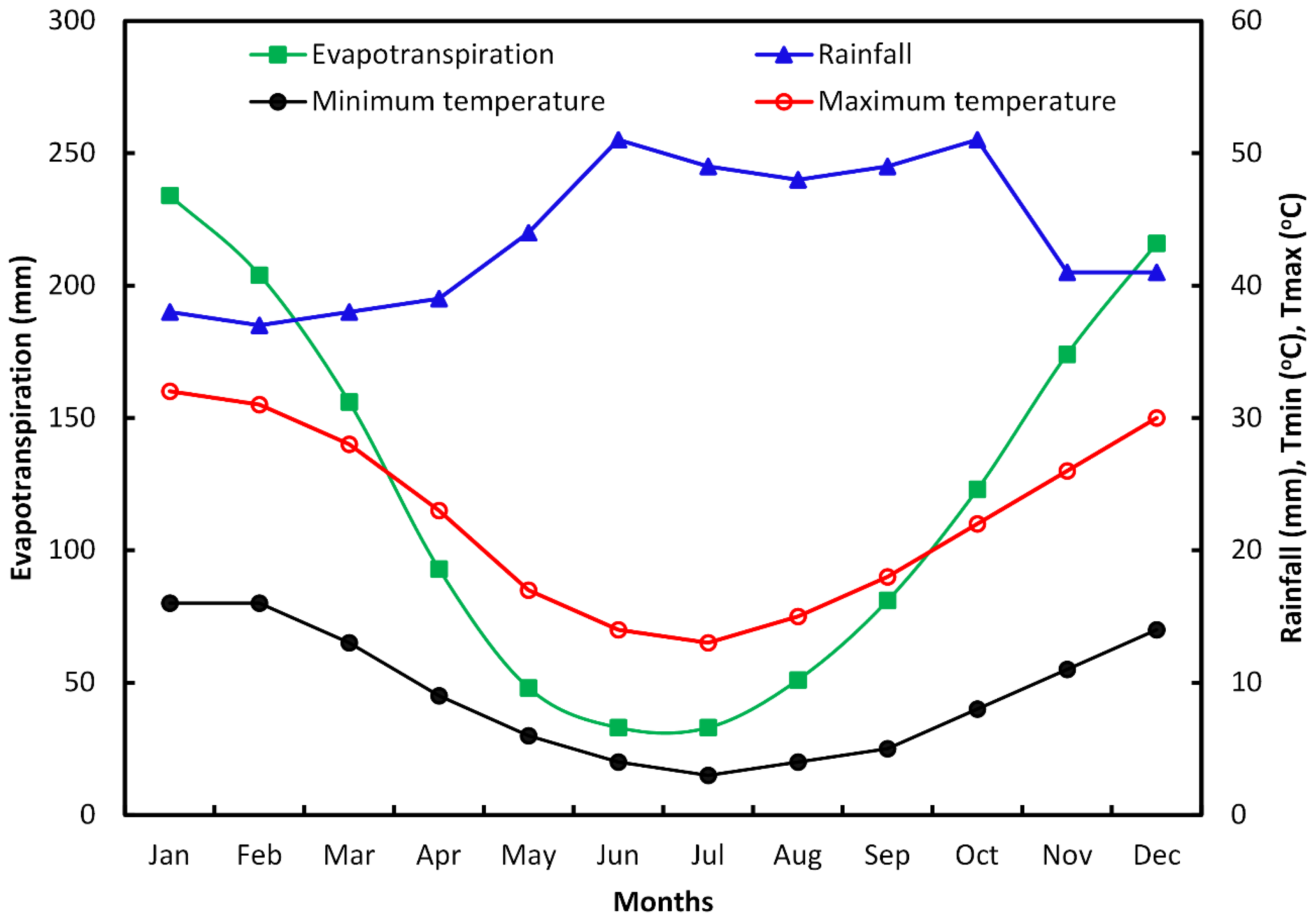
2.4. Weather Data
2.5. Brief Description of AquaCrop
2.6. AquaCrop Input Data
2.6.1. Crop Data
2.6.2. Weather Data
2.6.3. Soil Data
2.6.4. Management Decisions
2.7. Model Calibration and Testing
3. Results and Discussion
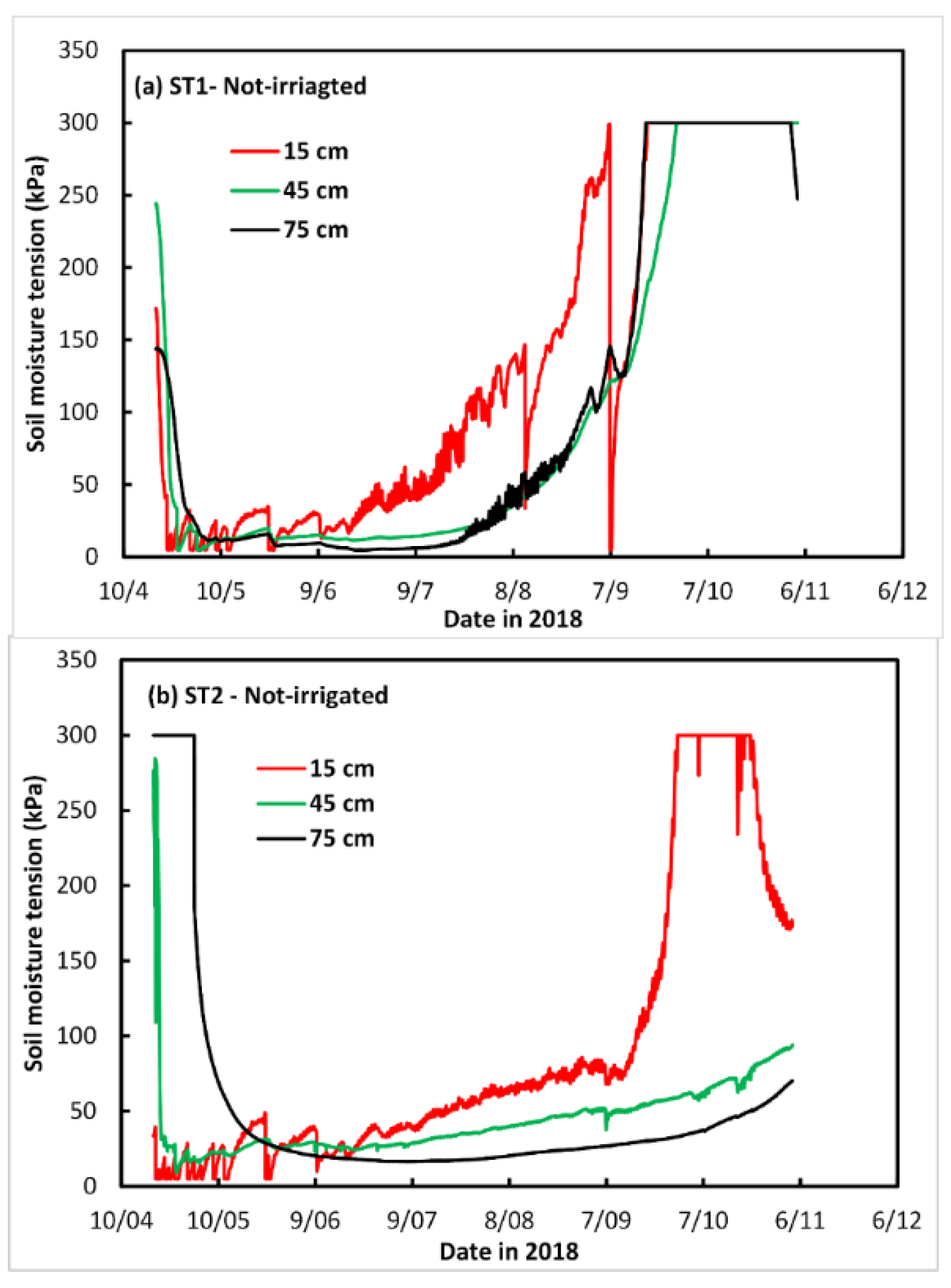
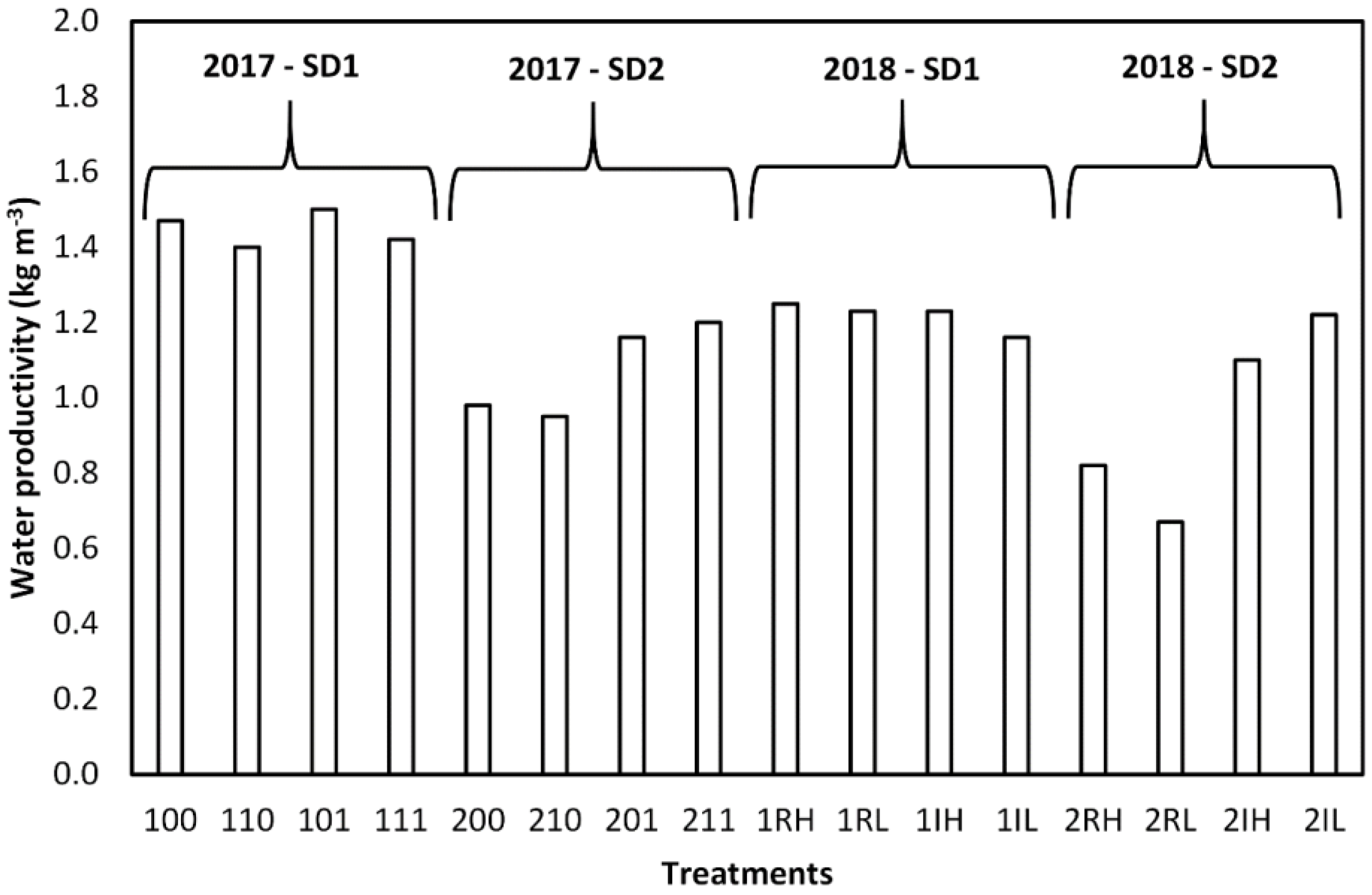
3.1. Rainfall, Irrigation, Evapotranspiration and Soil Water
3.2. Calibration for Soil Water Content, Green Canopy Cover, Above-Ground Dry Matter and Yield
3.3. Validation
3.3.1. Total Soil Water
3.3.2. Green Canopy Cover
3.3.3. Above-Ground Dry Matter and Grain Yield
3.4. Effect of Sowing Date
3.5. Response to Irrigation
3.6. Effect of Sowing Rate
4. Conclusions
Funding
Conflicts of Interest
References
- Grains Research and Development Cooperation. Faba Bean Southern Region—GrowerNotes; Grains Research and Development Cooperation: Canberra, Australia, 2017; Available online: https://grdc.com.au/resources-and-publications/grownotes/crop-agronomy/faba-bean-southern-region-grownotes (accessed on 22 February 2019).
- Zong, X.; Liu, X.; Guan, J.; Wang, S.; Liu, Q.; Paull, J.G. Molecular variation among Chinese and global winter faba bean germplasm. Theor. Appl. Genet. 2009, 118, 971–978. [Google Scholar] [CrossRef] [PubMed]
- Garofalo, P.; Di Paolo, E.; Rinaldi, M. Durum wheat (Triticum durum Desf.) in rotation with faba bean (Vicia faba var. minor L.): Long-term simulation case study. Crop Past. Sci. 2009, 60, 240–250. [Google Scholar] [CrossRef]
- Di Paolo, E.; Garofalo, P.; Rinaldi, M. Irrigation and nitrogen fertilization treatments on productive and qualitative traits of broad bean (Vicia faba var. minor L.) in a Mediterranean environment. Legume Res. 2015, 38, 209–218. [Google Scholar] [CrossRef]
- Siddiqui, M.H.; Al-Khaishany, M.Y.; Al-Qutami, M.A.; Al-Whaibi, M.H.; Grover, A.; Ali, H.M.; Al-Wahibi, M.S.; Bukhari, N.A. Response of Different Genotypes of Faba Bean Plant to Drought Stress. Int. J. Mol. Sci. 2015, 16, 10214–10227. [Google Scholar] [CrossRef] [PubMed] [Green Version]
- Mebrahtu, G.; Walelign, W.; Woldeyesus, S. Effect of Integrated Crop-Management Packages on Yield and Yield Components of Faba Bean (Vicia faba L.) cultivars in Southern Ethiopia. Vegetos Int. J. Plant Res. 2018, 31, 146–157. [Google Scholar] [CrossRef]
- Bishop, J.; Potts, S.G.; Jones, H.E. Susceptibility of faba bean (Vicia faba L.) to heat stress during floral development and anthesis. J. Agron. Crop Sci. 2016, 202, 202–508. [Google Scholar] [CrossRef] [PubMed]
- Flores, F.; Nadal, S.; Solis, I.; Winkler, J.; Sass, O.; Stoddard, F.L. Faba bean adaptation to autumn sowing under European climates. Agron. Sustain. Dev. 2012, 32, 727–734. [Google Scholar] [CrossRef] [Green Version]
- Adisarwanto, T.; Knight, R. Effect of sowing date and plant density on yield and yield components in the faba bean. Aust. J. Agric. Res. 1997, 48, 1161–1968. [Google Scholar] [CrossRef]
- Villalobos, F.J.; Orgaz, F.; Fereres, E. Sowing and Planting. In Agronomy for Sustainable Development; Villalobos, F., Fereres, E., Eds.; Springer: Cham, Switzerland, 2016. [Google Scholar]
- Keating, B.A.; Carberry, P.S.; Hammer, G.L. An overview of APSIM, a model designed for farming systems simulation. Eur. J. Agron. 2003, 18, 267–288. [Google Scholar] [CrossRef] [Green Version]
- Jones, J.W.; Hoogenboom, G.; Porter, C.H.; Boote, K.J.; Batchelor, W.D.; Hunt, L.A.; Wilkens, P.W.; Singh, U.; Gijsman, A.J.; Ritchie, J.T. The DSSAT cropping system model: Modelling cropping systems: Science, software and applications. Eur. J. Agron. 2003, 18, 235–265. [Google Scholar] [CrossRef]
- Falconnier, G.N.; Journet, E.P.; Bedoussac, L.; Vermue, A.; Chlébowski, F.; Beaudoin, N.; Justes, E. Calibration and evaluation of the STICS soil-crop model for faba bean to explain variability in yield and N 2 fixation. Eur. J. Agron 2019, 104, 63–77. [Google Scholar] [CrossRef]
- Ruiz-Ramos, M.; Mínguez, M.I. ALAMEDA, a structural-functional model for faba bean crops: Morphological parameterization and verification. Ann. Bot. 2006, 97, 377–388. [Google Scholar] [CrossRef] [PubMed]
- Hassanein, M.K.; Medany, M.A.; Haggag, M.E.; Bayome, S.S. Prediction of yield and growth of faba bean using CROPGRO legume model under egyptian conditions. Acta Hort. 2007, 729, 215–219. [Google Scholar] [CrossRef]
- Boote, K.J.; Mínguez, M.I.; Sau, F. Adapting the CROPGRO legume model to simulate growth of faba bean. Agron. J. 2002, 94, 743–756. [Google Scholar] [CrossRef]
- Raes, D.; Steduto, P.; Hsiao, T.C.; Fereres, E. AquaCrop—The FAO crop model to simulate yield response to water: II. Main algorithms and software description. Agron. J. 2009, 101, 438–447. [Google Scholar] [CrossRef]
- Bello, Z.A.; Walker, S. Calibration and validation of AquaCrop for pearl millet (Pennisetum glaucum). Crop Pasture Sci. 2016, 67, 948–960. [Google Scholar] [CrossRef]
- Trombetta, A.; Lacobellis, V.; Taranito, E.; Gentile, F. Calibration of the AquaCrop model for winter wheat using MODIS LAI images. Agric. Water Manag. 2016, 164, 304–316. [Google Scholar] [CrossRef]
- Nyathi, M.K.; van Halsema, G.E.; Annandale, J.G.; Struik, P.C. Calibration and validation of the AquaCrop model for repeatedly harvested leafy vegetables grown under different irrigation regimes. Agric. Water Manag. 2018, 208, 107–119. [Google Scholar] [CrossRef]
- García-Vila, M.; Fereres, E.; Mateos, L.; Orgaz, F.; Steduto, P. Deficit irrigation optimization of cotton with AquaCrop. Agron. J. 2009, 101, 477–487. [Google Scholar] [CrossRef]
- Heng, L.K.; Hsiao, T.; Evett, S.; Howell, T.; Steduto, P. Validating the FAO AquaCrop Model for Irrigated and Water Deficient Field Maize. Agron. J. 2009, 101, 488–498. [Google Scholar] [CrossRef] [Green Version]
- Abrha, B.; Delbecque, N.; Raes, D.; Tsegay, A.; Todorovic, M.; Heng, L.; Vanuytrecht, E.; Geerts, S.; Garcia-Vila, M.; Deckers, S. Sowing strategies for barley (Hordeum vulgare L.) based on modelled yield response to water with AquaCrop. Exp. Agric. 2012, 48, 252–271. [Google Scholar] [CrossRef]
- Zeleke, K.T.; Luckett, D.; Cowley, R. Calibration and testing of the FAO AquaCrop model for canola. Agron. J. 2011, 103, 1610–1618. [Google Scholar] [CrossRef]
- ApSoil. A Database of Soil Characteristics. 2013. Available online: http://www.apsim.info/Products/APSoil.aspx (accessed on 15 January 2019).
- Pulse Australia. PBA Samira Faba Bean. Southern Region. Pulse Australia. 2014. Available online: http://pulseaus.com.au/storage/app/media/crops/2014_VMP-Fababean-PBASamira.pdf (accessed on 12 March 2019).
- Perry, E.M.; Fitzgerlad, G.J.; Poole, N.; Craig, S.; Whitlock, A. Ndvi from active optical sensors as a measure of canopy cover and biomass. In International Archives of the Photogrammetry, Remote Sensing and Spatial Information Sciences; ISPRS Congress: Melbourne, Australia, 2012; p. 8. [Google Scholar]
- Steduto, P.; Hsiao, T.C.; Raes, D.; Fereres, E. AquaCrop—The FAO crop model to simulate yield response to water: I. Concepts and underlying principles. Agron. J. 2009, 101, 426–437. [Google Scholar] [CrossRef]
- Allen, R.G.; Pereira, L.S.; Raes, D.; Smith, M. Crop Evapotranspiration. Guidelines for Computing Crop Water Requirements; Irrigation and Drainage Paper No. 56; FAO: Rome, Italy, 1998. [Google Scholar]
- Willmott, C.J. Some comments on the evaluation of model performance. Bull. Am. Meteorol. Soc. 1982, 63, 1309–1313. [Google Scholar] [CrossRef]
- Steduto, P.; Hsiao, T.C.; Fereres, E. On the conservative behaviour of biomass water productivity. Irrig. Sci. 2007, 25, 189–207. [Google Scholar] [CrossRef]
- Richards, M.; Armstrong, E.; Gaynor, L.; Graham, N.; Coombes, N. Sowing Time and Variety Selection for Faba Bean in Southern NSW. Grains Research and Development Cooperation GRDC. 2016. Available online: https://grdc.com.au/resources-and-publications/grdc-update-papers/tab-content/grdc-update-papers/2016/02/sowing-time-and-variety-selection-for-faba-bean-in-southern-nsw (accessed on 17 March 2019).
- Matthews, P.; McCaffery, D.; Jenkins, L. Winter Crop Variety Sowing Guide 2017; NSW Department of Primary Industries: Sydney, Australia, 2017. [Google Scholar]
- Pulse Australia. Faba Bean Production: Southern and Western Region. Pulse Australia. 2016. Available online: http://www.pulseaus.com.au/growing-pulses/bmp/faba-and-broad-bean/southern-guide#general-agronomy (accessed on 17 March 2019).
- Martini, L.C.P. Sensitivity analysis of the AquaCrop parameters for rainfed corn in the South of Brazil. Pesq. Agropec. Bras. 2018, 53, 934–942. [Google Scholar] [CrossRef]
- Gebert, C.; Midwood, J. Faba Bean Agronomy. Southern Farming System. 2016. Available online: http://www.sfs.org.au/trial-result-pdfs/Trial_Results_2016_VIC/5.7%20Faba%20bean%20agronomy.pdf (accessed on 12 April 2019).


| Soil Depth (cm) | ρb (g cm−3) | LL15 (cm3 cm−3) | DUL (cm3 cm−3) | Sat (cm3 cm−3) | ECe (µScm−1) | PH (unit) | OrgC (%) |
|---|---|---|---|---|---|---|---|
| 0–15 | 1.48 | 0.11 | 0.29 | 0.35 | 42 | 7.6 | 1.22 |
| 15–30 | 1.50 | 0.13 | 0.27 | 0.34 | 44 | 7.4 | 0.72 |
| 30–45 | 1.45 | 0.15 | 0.25 | 0.32 | 43 | 7.4 | 0.35 |
| 45–60 | 1.37 | 0.15 | 0.28 | 0.36 | 69 | 6.7 | 0.37 |
| 60–90 | 1.43 | 0.15 | 0.29 | 0.35 | |||
| 90–120 | 1.55 | 0.15 | 0.31 | 0.34 |
| Treatments | Year 1 | Treatments | Year 2 | ||
|---|---|---|---|---|---|
| Rainfall (mm) | Irrigation (mm) | Rainfall (mm) | Irrigation (mm) | ||
| 100 | 219 | 0 | 1RL | 149 | 0 |
| 110 | 219 | 61 | 1RH | 149 | 0 |
| 101 | 219 | 107 | 1IL | 149 | 250 |
| 111 | 219 | 246 | 1IH | 149 | 250 |
| 200 | 269 | 0 | 2RL | 165 | 0 |
| 210 | 269 | 31 | 2RH | 165 | 0 |
| 201 | 269 | 107 | 2IL | 165 | 187 |
| 211 | 269 | 207 | 2IH | 165 | 187 |
| Grain Yield (t ha−1) | Total Soil Water (mm) | Green Canopy Cover (%) | Above-Ground Dry Matter (t ha−1) | |||||||||||||
|---|---|---|---|---|---|---|---|---|---|---|---|---|---|---|---|---|
| Year | Treatment | M (t ha−1) | S (t ha−1) | Dev (%) | R2 | d | RMSE (mm) | NRMSE (%) | R2 | d | RMSE (%) | NRMSE (%) | R2 | d | RMSE | NRMSE (%) |
| 2017 | SD1-NI | 3.65 | 4.41 | 17 | 0.86 | 0.70 | 33.3 | 15.1 | 0.83 | 0.88 | 19.8 | 45.6 | 0.94 | 0.94 | 2.9 | 42.8 |
| 2017 | SD1-RI | 5.85 | 5.55 | −5 | 0.83 | 0.86 | 16.5 | 7.3 | 0.88 | 0.94 | 15.1 | 29.8 | 0.96 | 0.88 | 4.7 | 56.6 |
| 2017 | SD1-VI | 3.97 | 4.46 | 11 | 0.88 | 0.81 | 27.0 | 12.8 | 0.92 | 0.93 | 14.2 | 29.1 | 0.98 | 0.91 | 3.7 | 46.9 |
| 2017 | SD1-FI | 5.24 | 5.14 | −2 | 0.85 | 0.95 | 9.4 | 4.1 | 0.83 | 0.96 | 11.9 | 21.8 | 0.96 | 0.94 | 3.1 | 40.1 |
| 2017 | SD2-NI | 2.32 | 2.57 | 10 | 0.90 | 0.80 | 31.6 | 14.9 | 0.85 | 0.82 | 12.4 | 23.3 | 0.98 | 0.97 | 0.9 | 24.4 |
| 2017 | SD2-RI | 5.24 | 4.92 | −7 | 0.79 | 0.79 | 28.1 | 12.3 | 0.90 | 0.93 | 17.2 | 52.2 | 0.94 | 0.96 | 1.4 | 30.1 |
| 2017 | SD2-VI | 3.02 | 3.58 | 16 | 0.92 | 0.82 | 30.3 | 14.3 | 0.98 | 0.98 | 8.9 | 25.7 | 0.94 | 0.96 | 1.1 | 27.2 |
| 2017 | SD2-FI | 5.52 | 5.20 | −6 | 0.92 | 0.93 | 15.3 | 6.6 | 0.98 | 0.97 | 12.4 | 33.7 | 0.92 | 0.91 | 2.3 | 43.2 |
| 2018 | SD1-IH | 4.64 | 4.10 | −13 | 0.88 | 0.96 | 10.1 | 4.4 | 0.96 | 0.98 | 8.0 | 11.1 | 0.98 | 0.96 | 2.7 | 32.8 |
| 2018 | SD1-IL | 4.89 | 4.10 | −11 | 0.92 | 0.91 | 14.1 | 6.3 | 0.94 | 0.91 | 9.9 | 13.5 | 0.96 | 0.94 | 3.4 | 40.6 |
| 2018 | SD1-NIH | 3.23 | 3.27 | 1 | 0.98 | 0.90 | 21.3 | 9.8 | 0.88 | 0.84 | 13.4 | 18.3 | 0.88 | 0.87 | 4.9 | 55.9 |
| 2018 | SD1-NIL | 3.15 | 3.27 | 4 | 0.98 | 0.94 | 17.9 | 8.2 | 0.85 | 0.83 | 13.4 | 18.9 | 0.92 | 0.92 | 3.7 | 45.9 |
| 2018 | SD2-IH | 4.33 | 3.64 | −19 | 0.96 | 0.96 | 12.3 | 5.5 | 0.74 | 0.93 | 15.0 | 31.6 | 0.96 | 0.92 | 2.3 | 36.7 |
| 2018 | SD2-IL | 4.18 | 4.00 | −4 | 0.92 | 0.94 | 15.4 | 6.7 | 0.92 | 0.92 | 16.5 | 31.3 | 0.96 | 0.95 | 1.6 | 27.3 |
| 2018 | SD2-NIH | 2.04 | 1.69 | −21 | 0.81 | 0.83 | 29.9 | 16.1 | 0.52 | 0.74 | 21.8 | 47.5 | 0.92 | 0.97 | 0.8 | 19.2 |
| 2018 | SD2-NIL | 2.08 | 1.73 | −20 | 0.85 | 0.78 | 26.8 | 10.5 | 0.66 | 0.84 | 15.7 | 39.6 | 0.92 | 0.85 | 2.7 | 45.8 |
| Average | 3.96 | 3.85 | −3 | 0.89 | 0.87 | 21.2 | 9.7 | 0.85 | 0.90 | 14.1 | 29.6 | 0.95 | 0.93 | 2.6 | 38.4 | |
| R2 | 0.86 | |||||||||||||||
| d | 0.95 | |||||||||||||||
| RMSE | 0.49 | |||||||||||||||
| NRMSE | 12.4 | |||||||||||||||
| Base temperature (°C) | 0 |
| Upper temperature (°C) | 30 |
| Cover per seedling (cm2 plant−1) | 5 |
| Canopy growth coefficient CGC (% GDD−1) | 0.701 |
| Canopy decline coefficient CDC (% GDD−1) | 0.697 |
| Soil water depletion factor for canopy expansion, upper limit | 0.25 |
| Soil water depletion factor for canopy expansion, lower limit | 0.65 |
| Shape factor for water stress coefficient for canopy expansion | 3.0 |
| Soil water depletion factor for stomatal closure | 0.5 |
| Shape factor for water stress coefficient for stomatal closure | 3.0 |
| Soil water depletion factor for early canopy senescence | 0.50 |
| Shape factor for water stress coefficient for canopy senescence | 4.0 |
| Normalized water productivity WP* (g m−2) | 18 |
| Adjustment for yield formation (%) | 100 |
| Initial canopy cover CCo (%) | 1.2 |
| Maximum canopy cover CCx (%) | 90 |
| Time to maximum canopy cover (GDD) | 1200 |
| Time to flowering (GDD) | 1290 |
| Length of the flowering stage (GDD) | 557 |
| Time to senescence (GDD) | 1845 |
| Time to maturity (GDD) | 2380 |
| Rooting depth (m) | 0.90 |
| Reference harvest index HIo (%) | 40 |
© 2019 by the author. Licensee MDPI, Basel, Switzerland. This article is an open access article distributed under the terms and conditions of the Creative Commons Attribution (CC BY) license (http://creativecommons.org/licenses/by/4.0/).
Share and Cite
Zeleke, K.T. AquaCrop Calibration and Validation for Faba Bean (Vicia faba L.) under Different Agronomic Managements. Agronomy 2019, 9, 320. https://doi.org/10.3390/agronomy9060320
Zeleke KT. AquaCrop Calibration and Validation for Faba Bean (Vicia faba L.) under Different Agronomic Managements. Agronomy. 2019; 9(6):320. https://doi.org/10.3390/agronomy9060320
Chicago/Turabian StyleZeleke, Ketema Tilahun. 2019. "AquaCrop Calibration and Validation for Faba Bean (Vicia faba L.) under Different Agronomic Managements" Agronomy 9, no. 6: 320. https://doi.org/10.3390/agronomy9060320