Article

Identification of Robust Hybrid Inversion Models on the Crop Fraction of Absorbed Photosynthetically Active Radiation Using PROSAIL Model Simulated and Field Multispectral Data

College of Hydraulic Science and Engineering, Yangzhou University, Yangzhou 225009, China
*
Author to whom correspondence should be addressed.
Agronomy 2023, 13(8), 2147; https://doi.org/10.3390/agronomy13082147
Submission received: 30 June 2023 / Revised: 5 August 2023 / Accepted: 14 August 2023 / Published: 16 August 2023
(This article belongs to the Special Issue Precision Agriculture Monitoring Using Remote Sensing)

Abstract

:
The fraction of absorbed photosynthetically active radiation (FPAR), which represents the capability of vegetation-absorbed solar radiation to accumulate organic matter, is a crucial indicator of photosynthesis and vegetation growth status. Although a simplified semi-empirical FPAR estimation model was easily obtained using vegetation indices (VIs), the sensitivity and robustness of VIs and the optimal inversion method need to be further evaluated and developed for canola FPAR retrieval. The objective of this study was to identify the robust hybrid inversion model for estimating the winter canola FPAR. A field experiment with different sow dates and densities was conducted over two growing seasons to obtain canola FPARs. Moreover, 29 VIs, two machine learning algorithms and the PROSAIL model were incorporated to establish the FPAR inversion model. The results indicate that the OSAVI, WDRVI and mSR had better capability for revealing the variations of the FPAR. Three parameters of leaf area index (LAI), solar zenith angle (SZA) and average leaf inclination angle (ALA) accounted for over 95% of the total variance in the FPARs and OSAVI exhibited a greater resistance to changes in the leaf and canopy parameters of interest. The hybrid inversion model with an artificial neural network (ANN-VIs) performed the best for both datasets. The optimal hybrid inversion model of ANN-OSAVI achieved the highest performance for canola FPAR retrieval, with R2 and RMSE values of 0.65 and 0.051, respectively. Finally, the work highlights the usefulness of the radiation transfer model (RTM) in quantifying the crop canopy FPAR and demonstrates the potential of hybrid model methods for retrieving the canola FPAR at each growth stage.

1. Introduction

The FPAR is the ratio of photosynthetically active radiation absorbed by the green part of the vegetation canopy to total photosynthetically active radiation (PAR) within the wavelength range of 400–700 nm. It is an important parameter for describing vegetation photosynthesis and physiological characteristics [1]. Since the 1990s, the FPAR has been extensively used in various areas, including assessing vegetation productivity [2], guiding vegetation growth management [3], and diagnosing drought and climate change [4]. Moreover, the FPAR has been recognized as one of the key climate variables that influence global climate change according to the Global Climate Observation System (GCOS) [5]. Therefore, accurate and reliable FPAR acquisition is of great significance for depicting terrestrial ecosystem processes and estimating crop yields [6].
FPAR estimation methods are usually divided into two categories: empirical methods based on vegetation indices (VIs) and physical model inversion based on the radiation transfer model (RTM). Vegetation indices can quantify the absorption and reflection of solar radiation by a vegetation canopy and are widely used for estimating the FPAR due to their fewer parameters and high computational efficiency [7]. Over the past few decades, numerous Vis, such as the normalized difference VI (NDVI) [8], enhanced VI (EVI) [9] and simple ratio index (SR) [10], have been developed, evaluated and shown to be effective in estimating the FPARs for various vegetation types. However, there are still several issues associated with the VI approach that need to be addressed. First, while VIs can reveal the physiological and ecological characteristics of vegetation, they cannot fully capture the changes in solar effective radiation within the canopy and surface [11,12]. Furthermore, estimating VIs introduced uncertainty due to factors like variations in solar elevation angle and soil background. Moreover, most VI methods were statistically based and exhibited different relationships between VIs and FPARs for various spatial and temporal vegetation dynamics, resulting in regional restrictions in their application. Glenn et al. [13] suggested that VIs could be simply used to determine canopy light absorption without involving the canopy structural level.
In contrast, the RTM could elucidate and simulate the process of FPAR change by incorporating explicit geometric models of the canopy structure [14]. Meng et al. [15] quantitatively retrieved the spatial distribution of the absorbed FPAR in salt marsh vegetation from satellite images using the soil–canopy–photochemical and energy flux observation coupling model (SCOPE). Liu et al. [16] employed the modified simultaneous heat and water radiation model (MSHAW) to simulate the vertical profile of FPAR within the canopy. The RTM demonstrated greater adaptability to diverse environments and background conditions for FPAR simulation, but the model uncertainties associated with the input parameters also affected the RTM accuracy. Computational technology advances, more optimization algorithms (e.g., gradient methods, genetic algorithms and simulated annealing) and machine learning algorithms (artificial neural networks (ANNs), support vector regression (SVR) and random forest (RF)) have been combined with RTMs to improve the FPAR inversion accuracy [17,18]. For example, Verger et al. [19] used the PROSAIL model in conjunction with a neural network algorithm to investigate a series of measured crop FPARs and model the simulated FPARs.
In addition to the mechanism-based inversion model, other studies also evaluated robust estimation models through sensitivity analysis, which investigates the impacts of parameter variations on simulation results (e.g., band reflectance and VI) [20,21]. For example, Leolini et al. [22] constructed the relationship between the rescaled VIs (NDVI, OSAVI, etc.) and the observed FPAR, and validated this relationship using independent datasets. Dong et al. [23] analyzed the sensitivity and correlation between the three modified VIs and the FPAR using reflectance data simulated by the PROSAIL model. However, most sensitivity analyses of VIs primarily focus on their influence on LAI changes, and limited studies on FPAR changes have been reported. Although LAI and FPAR are strongly correlated based on the Beer–Lambert law, the relationship is also modulated by the extinction coefficient, introducing a certain degree of uncertainty. Moreover, most previous studies focused on a single empirical or physical method, but few combined multiple methods for FPAR inversion. Hou et al. [24] used the PROSAIL model and a look-up table (LUT) algorithm to investigate the FPAR inversion from satellite data for different vegetation types in various regions. Kolassa et al. [25] proposed an empirical model calibration method to distinguish vegetation types based on the deviation between the simulated FPAR and MODIS-observed FPAR. Furthermore, studies on crop FPAR retrieval mainly focused on crops such as wheat, maize and soybean [26,27], but limited studies were performed on canola. Monitoring canola FPAR dynamics could effectively diagnose growth status and stage nodes, providing key variables for crop productivity models. Due to differences in the canopy structure between different crops, existing FPAR estimation models developed for other crops need further evaluation and validation when applied to canola [28,29].
Therefore, to identify the robust hybrid estimation methods for improving the canola FPAR retrieval accuracy, the PROSAIL model, which is a classical model mechanism of radiative transfer for vegetation canopy, was employed and recompiled to simulate FPAR variations. A total of 29 VIs and two machine learning algorithms were devoted to retrieving the FPAR. The model-estimated and in situ measured FPAR from a two-year field experiment were used to evaluate the inversion performance. The main objectives of this study were to (1) reveal the capability of different VIs in interpreting FPAR variation, (2) analyze the sensitivity of VIs to changes in leaf and canopy parameters, and (3) identify the robust hybrid estimation methods that consider inversion accuracy in different canola growth stages.

2. Materials and Methods
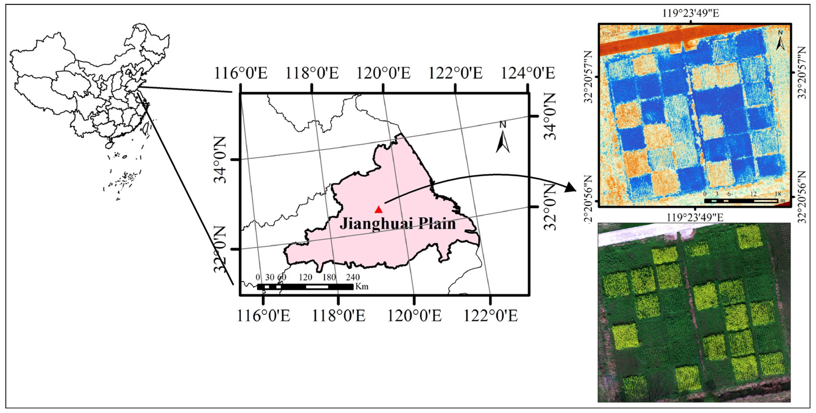
2.1. Study Area

From 2020–2022, a field experiment on canola was conducted at the Yangzijin Ecological Experimental Field of Yangzhou University. The experimental station was located in the middle of Jianghuai Plain, at coordinates 119°24′ E and 32°21′ N, with an elevation of 5 m above sea level and belonging to the subtropical monsoon climate zone (Figure 1). The annual average frost-free period, air temperature, evaporation and precipitation were 223 days, 14.8 °C, 937 mm and 1063 mm, respectively. The soil type in the experimental field was sandy loam, with pH value, field capacity, wilting point and bulk density of 8.14, 25%, 7.8% and 1.24 g cm−3, respectively. The initial nutrient contents in the top 20 cm of soil surface were as follows: organic matter 10.2 g kg−1, total nitrogen 0.97 g kg−1, available phosphorus 16.3 mg kg−1 and available potassium 151.2 mg kg−1 [30].

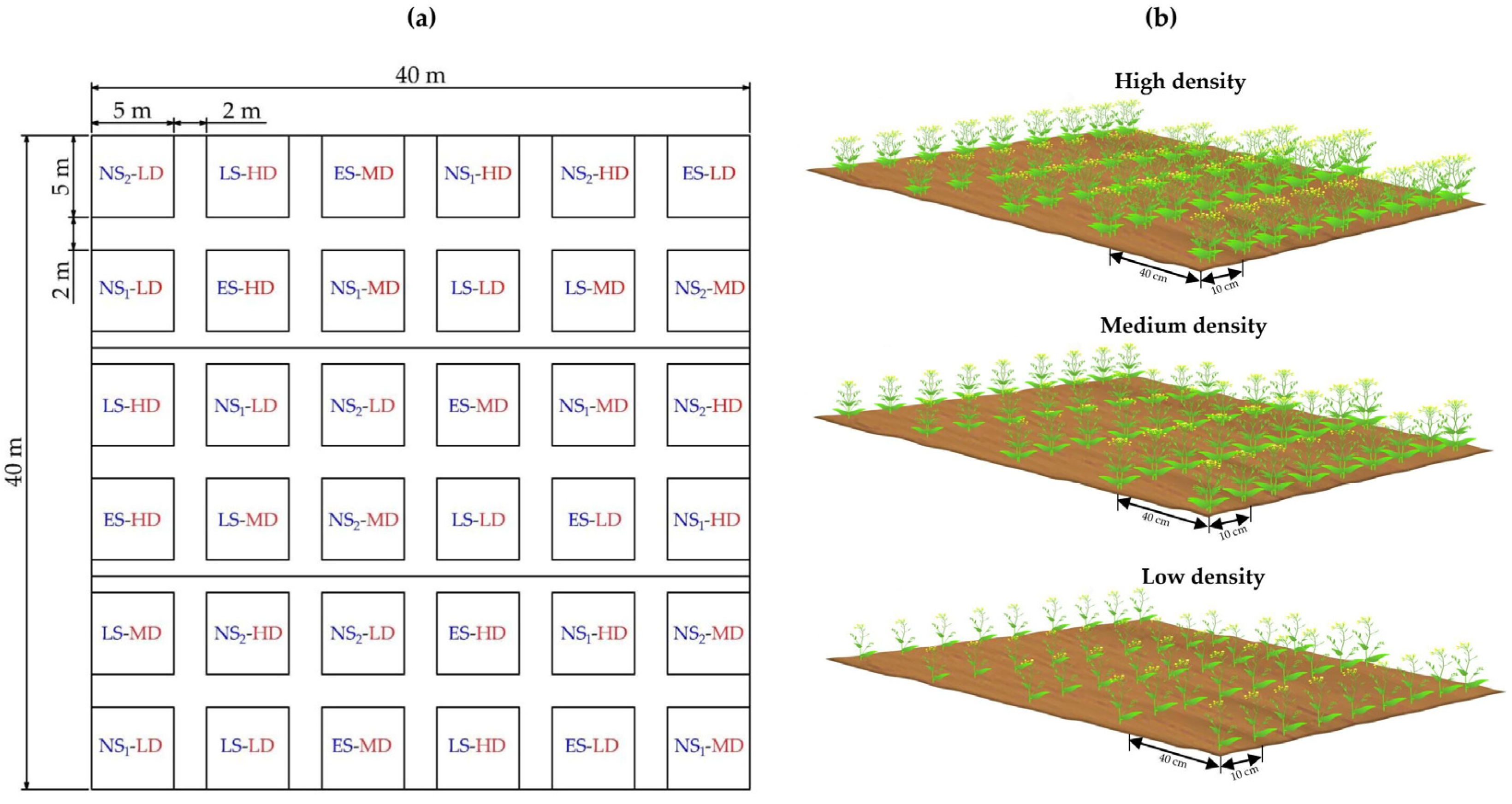
2.2. Experimental Design

In this experiment, the canola variety tested was “Deaiyou 558”. The 12 different sowing scenarios were designed and performed in the winter canola growing season (Figure 2). Referring to local practices, four sowing dates and three sowing densities were created to modulate the crop growth process. For the sowing date treatments, four periods denoted early (ES 21 September), normal (NS1 6 October, NS2 23 October) and late (LS 6 November) were chosen. Regarding the sowing density treatments, low (LD 12.5 plants m−2), medium (MD 25 plants m−2) and high densities (HD 37.5 plants m−2) were adopted. Thus, a total of 12 treatments and 36 plots (each treatment with three replicates) were established. Each plot area was 5 m × 5 m and the interval between adjacent plots was 2 m. The seeds were manually sown with a row spacing of 40 cm and a plant spacing of 10 cm. After the emergence of canola seedlings, the seedlings were thinned at the 3-leaf stage and the seedlings were fixed at the 5-leaf stage. Other field management practices, such as weeding, insecticide and disease prevention, followed the local field practices.

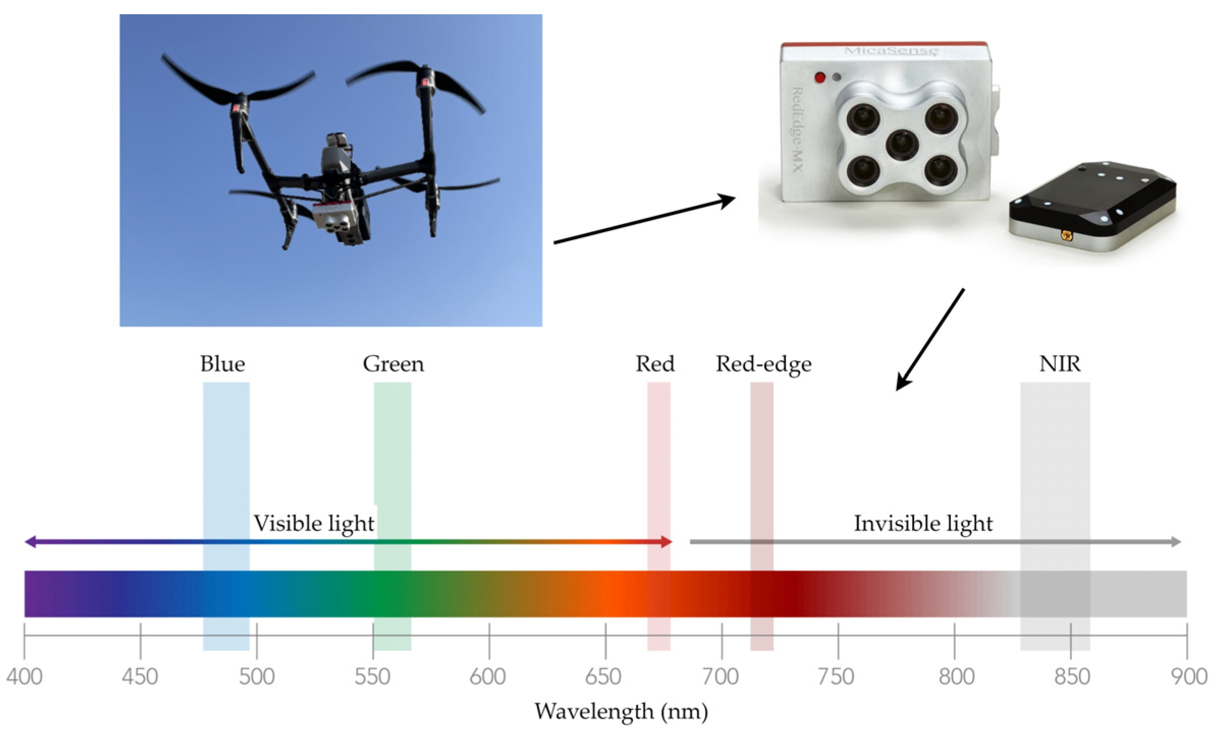
2.3. Canopy Multispectral Image Acquisition

During the growth period of the canola, multispectral images were obtained using the Rededge-mx multi-spectrometer (MicaSense, Inc., Seattle, WA, USA), which was mounted on a DJI Inspire 2 UAV remote sensing platform (DJI Inc., Shenzhen, China) (Figure 3). The spectral images were captured approximately 7–10 days after sowing, and the UAV remote sensing operation was carried out from 11 am to 1 pm, specifically in sunny and windless weather conditions. During each flight, five images with a resolution of 1280 × 960 pixels were obtained, corresponding to the blue (475 nm), green (560 nm), red (668 nm), red edge (717 nm) and near-infrared (840 nm) bands. During each flight operation, images of a reference plate were synchronously captured for radiation calibration. The flight height during the operation was set at 20 m, with an along- and cross-track overlap of 75%. The camera lens was pointed in the downward direction, capturing multispectral images with a ground resolution of 1.4 cm at a field of view of 47.2°. After each flight, the raw images were automatically processed using Pix4Dmapper software, including camera optimizing, photo aligning, radiometric correction and orthomosaic building. Finally, image reflectance data for each pixel throughout crop growth seasons were generated. For each plot, the average band reflectance was extracted using the selected region of interest (ROI) that excluded two rows of canola from the boundary area to avoid interference from plot edge effects, where crops grew more vigorously due to better lighting, ventilation and population competition.

2.4. Canopy FPAR Measurements

The canola canopy FPAR measurements were performed after the UAV image acquisition using the LP-80 PAR/LAI Ceptometer (AccuPAR, Decagon Devices Inc., Pullman, WA, USA). The LP-80 probe contained 80 independent sensors, which were evenly spaced 1 cm apart. The photosensors measured the PAR in the 400 to 700 nm waveband (μmol/(m2s)). During the FPAR measurement, the probe was placed along the row direction within the canopy. Four positions and directions were considered to obtain comprehensive PAR data, i.e., the incident PAR, the top of canopy reflected PAR, the bottom of canopy transmission PAR and the bottom of soil reflection PAR. Each plot was repeated five times to calculate the average value and the canola canopy FPAR was then calculated using Equation (1) [31]. A summary of the statistics of the canola FPAR acquired in situ is given in Table 1.
FPAR = ( I c I c   ( I uc     I uc ) ) I c
where Ic↓ is the solar downward radiation at the canopy top, Ic↑ is the solar radiation emitted from the canopy, Iuc↓ is the solar downward radiation under the canopy and Iuc↑ is the solar radiation reflected by the soil under the canopy.

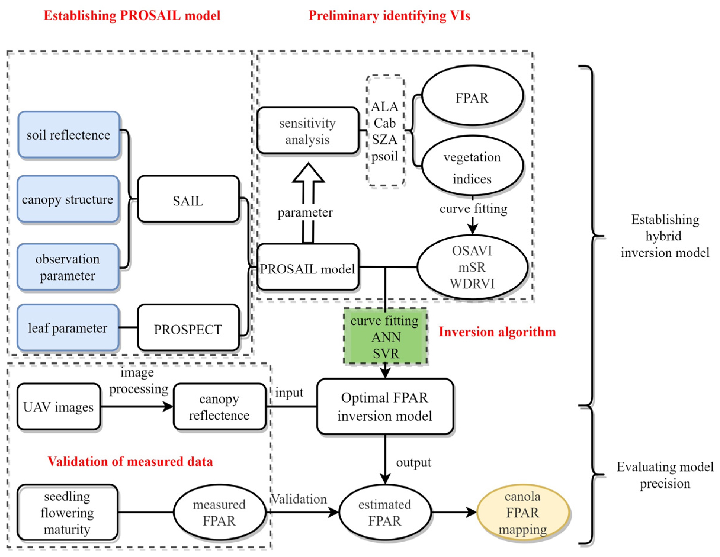
2.5. PROSAIL RTM and Data Simulation

To investigate the optimal inversion method for estimating the FPAR based on the RTM, the crop canopy spectra were simulated using the PROSAIL model. The primary PROSAIL model was proposed by Baret et al. [32], who coupled the PROSPECT leaf optical properties model [33] with the SAIL canopy bidirectional reflectance model [34] to describe the variations in the canopy spectral reflectance as a function of the biochemistry and architecture parameters. At the leaf level, the PROSPECT model parameters included leaf chlorophyll a + b content (Cab), carotenoid content (Car), brown pigment content (Cbrown), equivalent water thickness (Cw), dry matter content (Cm) and leaf internal structure parameter (N). For the canopy level, the SAIL model parameters included the LAI, ALA, hot spot size parameters (hspot), SZA, observer zenith angle (OZA), relative azimuth angle (psi) and soil brightness parameters (psoil).
In general, the canopy structure parameters (e.g., LAI, SZA, ALA and psoil), as well as the leaf-level parameters (Cab and N), have been found to have an effect on the FPAR variation [12,35]. According to the prior information, the LAI, Cab, ALA and SZA were identified as particularly influential factors that affect the FPAR. To explore the effects of different parameters and ranges on the FPAR, two simulated datasets were generated. One was a general dataset parameter distribution according to the literature [36,37,38]. Based on prior information and the previous research results of Dong et al. [39], the specific dataset for canola was determined by reducing the value range and step size of the canopy structure parameters (e.g., Cab and LAI) and illumination parameter (SZA). The parameter ranges and specific meanings within the PROSAIL model for both datasets are shown in Table 2.
The FPAR could be derived by combining the law of conservation of energy with the PROSAIL model [40]. First, the leaf reflectance and transmittance were obtained using the PROSPECT part of the PROSAIL model. Second, the multiple scattering effect caused by the interaction between the canopy and background soil was partially accounted for by the SAIL component of the PROSAIL model. Finally, the canopy FPAR was solved by calculating both the direct and scattered PAR. The total FPAR, direct FPAR and diffuse FPAR were calculated using the following Equations (2)–(6):
α s * =   α s + τ ss r sd + τ sd r dd 1   r dd ρ dd b α d
α d * =   α d + τ dd r dd 1   r dd ρ dd b α d
α s = 1 ρ sd τ sd τ ss
α d = 1   ρ dd τ dd
FPAR = λ = 400 λ = 700 ( α s * E dir t + α d * E dif t ) λ = 400 λ = 700 ( E dir t + E dif t ) = FPAR dir + FPAR dif
where α s * and α d * are the canopy absorptance for direct solar incident flux and hemispherical diffuse incident flux, respectively; α s and α d are the isolated canopy layer absorptance for direct solar incident flux and hemispherical diffuse incident flux respectively; τ ss and τ sd are the direct and bi-hemispherical transmittance for solar flux respectively; τ dd is the bi-hemispherical transmittance; r s d is the directional-hemispherical reflectance factor for solar incident flux and r dd is the bi-hemispherical reflectance factor; ρ sd and ρ dd are the directional-hemispherical reflectance for solar flux and bi-hemispherical reflectance above the canopy, respectively; ρ dd b is the bi-hemispherical reflectance at the bottom of the canopy; and E dir t and E dif t are the direct PAR and diffuse PAR, respectively.

2.6. Vegetation Indices (VIs)

Based on the simulated and measured canopy spectral data, a total of 29 VIs constructed using near-infrared and visible bands were selected (Table 3). The selected VIs, including the NDVI, SR and difference vegetation index (DVI), as well as modified indices, were employed to investigate the correlation between the FPAR and VIs. In order to identify the VIs suitable for FPAR estimation using general and specific simulation datasets, the first step was to establish the relationship between the simulated VIs and the FPAR by employing curve-fitting models, such as linear, exponential, power and logarithm models. The second step was to determine the major VIs that exhibited a good correlation with the FPAR using estimated error metrics. Subsequently, the VIs were evaluated by calculating the rank sum and arranging them in ascending order accordingly.

2.7. Sensitivity Analysis

To evaluate the influence of various leaf and canopy parameters on the variability of the FPAR, a global sensitivity analysis based on the extended Fourier amplitude sensitivity test (EFAST) algorithm was conducted. The EFAST is a variance-based global sensitivity analysis method that combines the computational efficiency of the classical FAST method with the global capability of the Sobol method. It is well-suited for nonlinear models, non-monotone models and interactions between parameters [68].
The EFAST analysis enabled the derivation of two indices: the first- and the total-order indices. The first-order index quantifies the individual contribution of each parameter to the overall variability, whereas the total-order index takes into account its interaction effect with other parameters. The 10,000 sample sets were generated based on the Monte Carlo method [69]. Subsequently, the FPAR was derived from the PROSAIL model and was then used to quantify the relative contribution of each model parameter.
In addition to the global sensitivity analysis, the local sensitivity of VIs to changes in the model parameters was further investigated. Appropriate VIs were not only sensitive to changes in the FPAR but also insensitive to other crop, soil and ambient factors. Hence, several sensitivity parameters determined beforehand using the EFAST method (e.g., LAI, SZA, ALA and psoil) were selected to evaluate the robustness of the VIs, while other insensitive parameters were kept fixed at the typical values (Table 2).

2.8. Inversion Modeling Algorithm

The regression relationship used in this study was established as an explicit parametric expression between the VIs and simulated FPAR from the PROSAIL model. The fitting functions could be linear or nonlinear (e.g., exponential or power function). Nonparametric algorithms, on the other hand, usually interpreted the strong nonlinearity of functional dependence between the biophysical/biochemical parameters and the spectral reflectance, such as ANN and SVR regression, which were more accurate and rational for the establishment of the inversion model. In this study, both the ANN and SVR algorithms were employed to establish a hybrid model with the selected VIs. For both the general and specific datasets, 80% of the samples were randomly extracted as the training (modeling) set, while the remaining samples were used for the model testing (validating) set. The process of establishing and validating hybrid inversion models based on the PROSAIL model and UAV images is presented in Figure 4.

2.8.1. The ANN Algorithm

The ANN algorithm mainly used the PROSAIL model as the training model and trained the ANN with the corresponding relationship between the canopy VIs and the FPAR. After the training, the top of the canopy reflectance extracted from the UAV images was used to evaluate the model performance. When applying the network model, the input layer was the VIs and the output layer was the FPAR. Training an ANN necessitated determining the network type and structure (i.e., the number of hidden layers and nodes per layer), and appropriately initializing the weights and regularization parameters to prevent overfitting. A two-layer feed-forward network with sigmoid hidden neurons and linear output neurons using the Levenberg–Marquardt algorithm was optimized. The ANN weights were randomly initialized according to the Nguyen–Widrow method, and a cross-validation procedure was implemented to mitigate overfitting [70].

2.8.2. The SVR Algorithm

The SVR is an empirical model based on a regression-type support vector machine, which can transform nonlinear regressions into linear ones by mapping the original low-dimensional input space into a higher-dimensional feature space based on various kernel functions [71]. To ensure its performance, the SVR required a training process that determined a set of model parameters by minimizing the generalization error. Predictions were done in the SVR by using an optimal hyperplane of a Gaussian radial basis kernel to minimize the prediction error. The kernel parameters (e.g., penalty and loss function) were determined via a grid search based on the least mean square error.

3. Results

3.1. Appropriate VIs for FPAR Estimation

To investigate the capability of VIs for interpreting the variations in the FPAR, the empirical regression models between different VIs and simulated FPAR based on two PROSAIL datasets are depicted in Table 4. The results indicate that the performances of different VIs for retrieving the FPAR varied across the two datasets, of which the parameter ranges were non-equivalent. Generally, the performance of the VIs could be summarized into four types of features. First, some VIs, like MCARVI, RDVIred-edge and MSAVI, presented good estimation performance for the general dataset but showed worse accuracies in the specific dataset, with a decline in R2 and an increase in RMSE. Contrarily, certain VIs (e.g., NDVI, RVI, SR and mNDVI) displayed superior regression model performance only with a specific dataset. The third type of VIs demonstrated stable and consistent model capabilities for both general and specific datasets, including OSAVI, WDRVI, mSR and OSAVIred-edge. Lastly, the remaining VIs exhibited poor model properties compared with the others, indicating that these limited the effectiveness of capturing the FPAR under common conditions. Therefore, considering the modeling signatures and accuracy ranking for both datasets, the top three VIs of OSAVI, WDRVI and mSR, which presented robustness and adaptableness among the 29 VIs, were identified as effective variables for further retrieving the crop FPAR.

3.2. Sensitivity Analysis

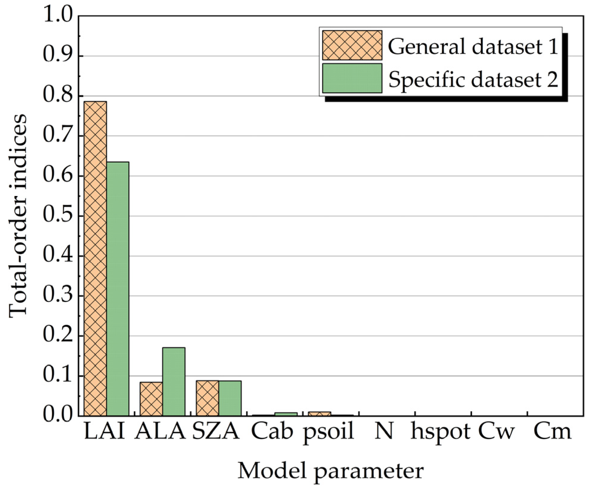
3.2.1. Global Sensitivity Analysis of the FPAR

A global sensitivity analysis was conducted using simulated canopy spectral data with the PROSAIL model and the EFAST algorithm to quantify the relative contributions of the leaf and canopy parameters to the variation in the FPAR (Figure 5). The results consistently indicated that the three parameters of LAI, SZA and ALA produced the dominant influences on the variability of the FPAR among the nine parameters of interest, accounting for over 95% of total variance. Cab and psoil ranked fourth and fifth, respectively, in terms of their contributions. Although there was a slight difference in the total-order indices between the general and specific datasets, LAI remained the greatest contributor to the variations in the FPAR. For the general dataset, the ALA and SZA jointly dominated the variability of the FPAR, making up about 10% of the variance, except for the LAI. Meanwhile, as the parameters distribution narrowed (specific dataset), the sensitivity index of the LAI decreased from 0.79 to 0.67, and the sensitivity of ALA increased from 0.08 to 0.17. Although the influences of Cab and psoil on the FPAR variation were relatively weak, they were still much higher than those of the other four parameters (i.e., N, Cm, hspot and Cw), of which the influences on the FPAR changes were less than one thousandth and could be considered negligible.

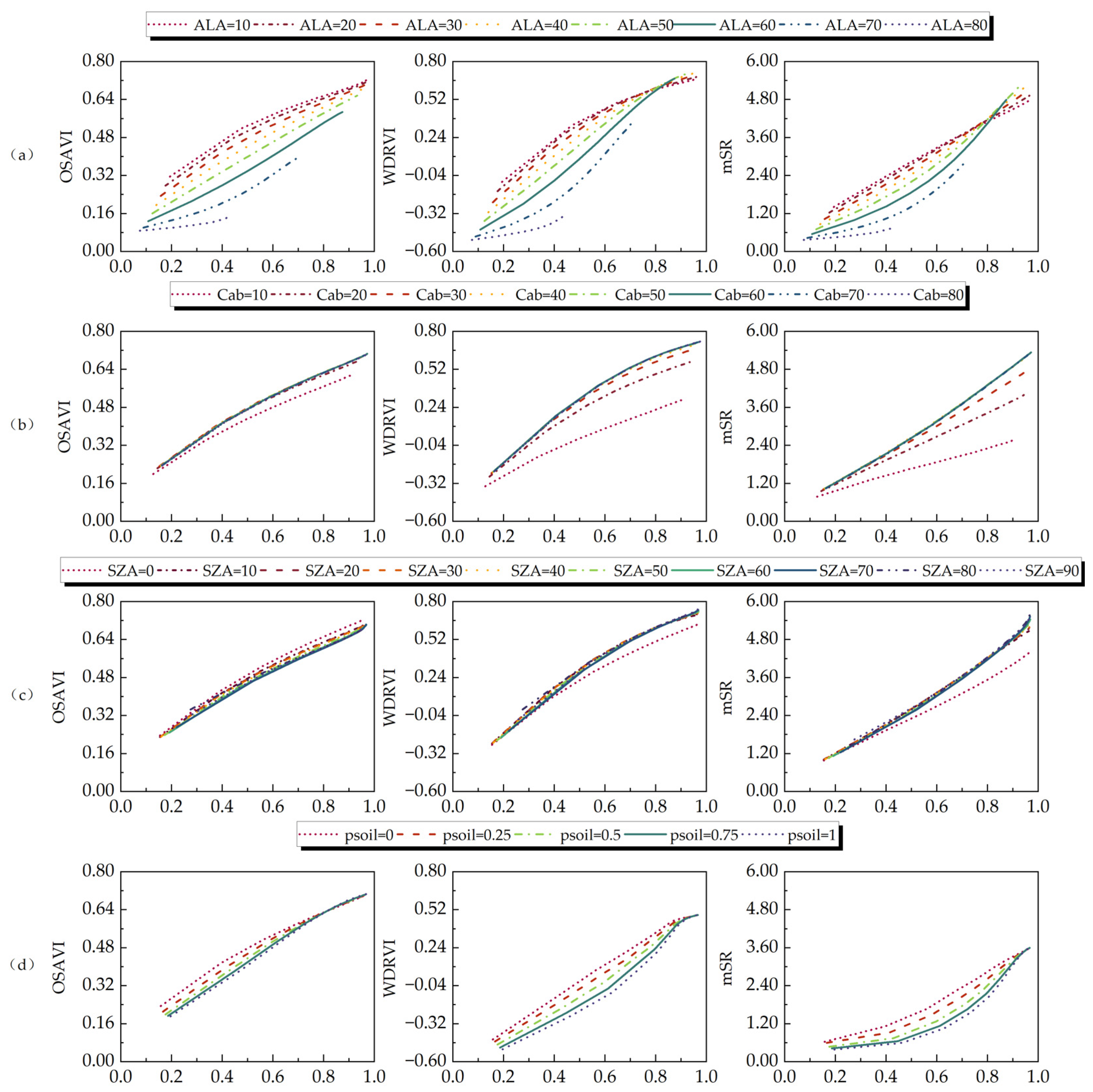
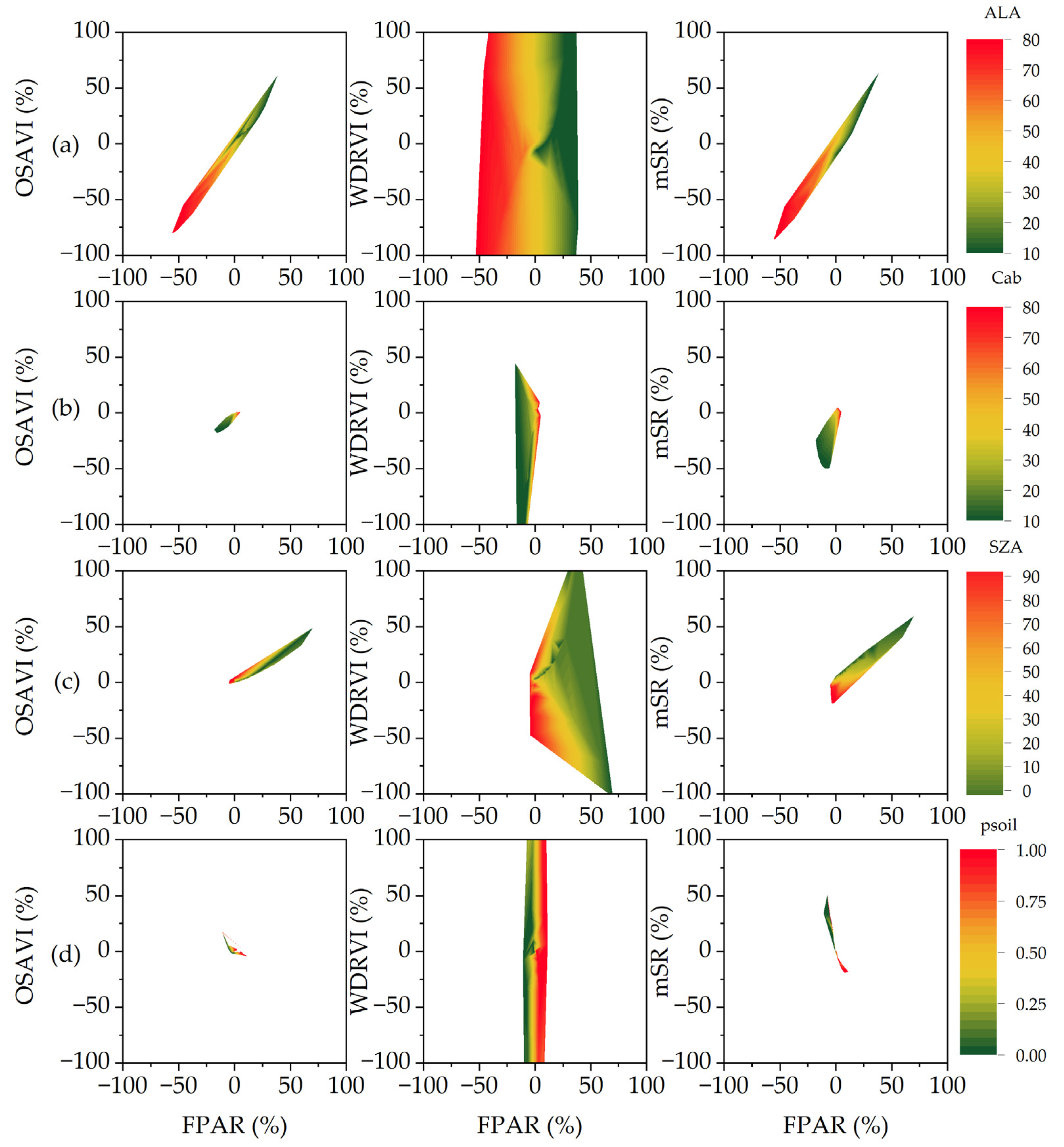
3.2.2. Local Sensitivity Analysis of the FPAR

In addition to the global sensitivity analysis, the variabilities of the VIs and FPAR as functions of each parameter were investigated as well. Theoretically, a robust VI should not only have a significant relationship with the target variable (FPAR) but also display resistance to changes in other variables. For the ALA parameter, the variations in ALA had a great influence on three VIs. The amount of canopy light interception decreased as ALA increased, resulting in a decline in the values of the VIs and FPAR (Figure 6a). A good linear regression between the VIs and FPAR could be observed when the ALA was less than 70°. Similar variabilities of OSAVI and mSR were achieved with increasing and decreasing ALA, but the WDRVI presented remarkable changes beyond −100% and 100% (Figure 7a).
The leaf chlorophyll content was another important indicator for considering the sensitivity of the VIs. Figure 6b and Figure 7b depict the variations in the VIs and FPAR with the Cab changes. In general, the VIs decreased with a drop in Cab due to an increase in the spectral reflectance of visible light. Compared with the mSR and WDRVI, the OSAVI presented excellent robustness for Cab changes. The relationships between OSAVI and FPAR were fully consistent in most cases, with variations only observed at a Cab of 10 μg cm−2. The VIs of mSR and WDRVI showed good robustness with higher Cab. Meanwhile, the sensitivities of mSR and WDRVI to Cab variations were significantly increased when Cab was lower than 30 μg cm−2. Substantial variations for mSR and WDRVI were noticed with a Cab of 10 μg cm−2, implying that the estimation accuracy was exacerbated during the crop maturity period when the leaves turned yellow.
The effects of SZA changes on three VIs were illustrated in Figure 6c and Figure 7c. The SZA had a minimal effect on the three VIs, except for slight changes at the lowest SZA (0°). Although the VIs presented a strong resistance to changes in SZA, the regressions between the VIs and FPAR were slightly different, with a high linear correlation with mSR and a nonlinear correlation with both OSAVI and WDRVI. These results indicated that the estimated FPAR suppressed the impact from SZA, which broke through the common time for capturing images at noon. The psoil was the important parameter in the PROSAIL, which could significantly influence the canopy spectral reflectance by controlling the soil brightness from dark (1) to bright (0). The variabilities in the VIs and FPAR in psoil are shown in Figure 6d and Figure 7d. The VIs would be decreased with the increase in psoil. A smaller amplitude of regression for the variation in psoil was observed in OSAVI and the sensitivity of the psoil parameter was decreased under a higher canopy cover (FPAR > 0.8). Compared with OSAVI, WDRVI and mSR exhibited more variability and weaker resistance to changes in psoil, particularly when the FPAR was between 0.4 to 0.6.

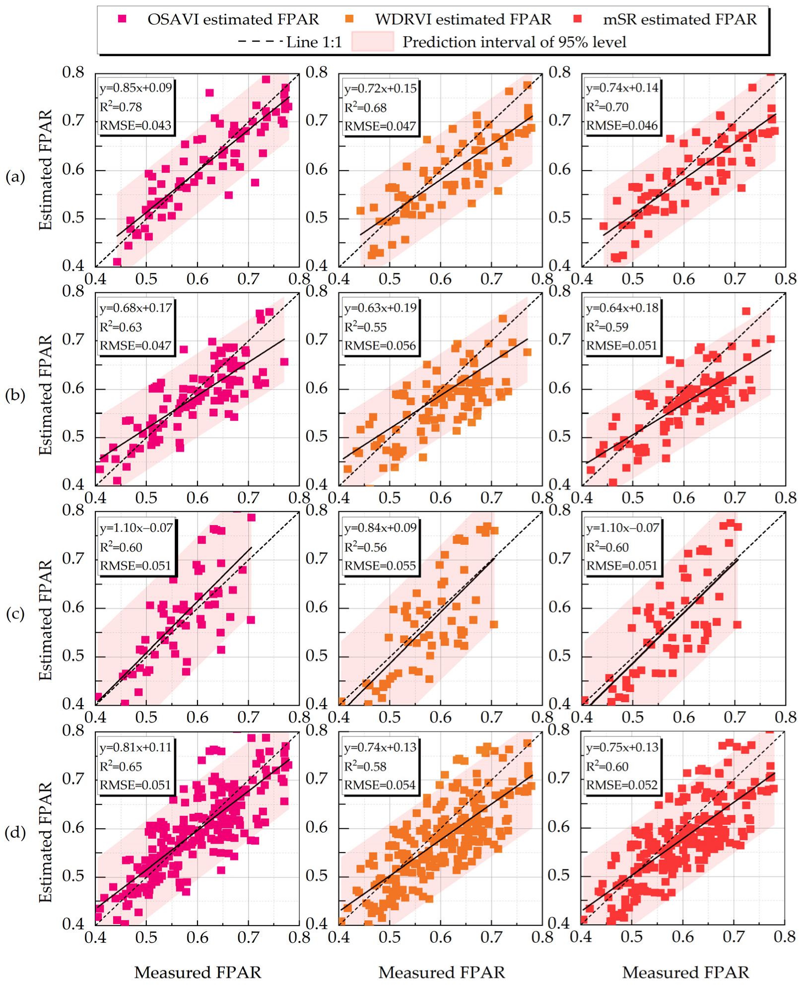
3.3. Performance of the Inversion Model with the Validation Dataset

Although the robustness results of the VIs of OSAVI, WDRVI and mSR for interpreting the variability in FPAR were given in the previous section, the performance of the optimal estimation model was unstable when applied to different datasets. Therefore, in order to address this issue, hybrid inversion models based on the ANN and SVR were established to explore the optimal estimation of FPAR. The inversion performances of these models are displayed in Table 5. Consistent results were achieved showing that OSAVI had better predictive capability than the other VIs for all three inversion methods, with an outstanding R2 and minimum RMSE. Among the three inversion methods, the ANN algorithm worked best, surpassing both the curve fitting and SVR methods. Overall, the ANN-OSAVI hybrid inversion model based on PROSAIL model data presented the optimal capability for estimating FPAR, with an R2 of 0.822 and RMSE of 0.055 for general dataset 1 and an R2 of 0.775 and RMSE of 0.059 for specific dataset 2.

3.4. Evaluation of the Optimal Inversion Model for Estimating Canola

Although the ANN-OSAVI-based hybrid model exhibited the optimal accuracy compared with WDRVI and mSR, the difference between the three hybrid models was minimal, from which it is challenging to determine the capability in estimating the canola FPAR due to potential discrepancies between the RTM model and real field conditions. Therefore, hybrid models of the ANN algorithm combined with three VIs were evaluated using the canola FPAR of each growing stage and the whole growing stages (Figure 8).
In general, the inversion accuracies of the hybrid model in the seedling stages were significantly higher than those in other stages. Similar trends were observed for the flowering and maturity stages. Specifically, for the seedling stage, ANN-OSVAI exhibited the highest accuracy, with R2 and RMSE values of 0.78 and 0.043, respectively. ANN-WDRVI and ANN-mSR also performed well but had slightly lower R2 values around 0.7 due to the discrete samples. Additionally, these models presented underestimated tendencies when the FPAR > 0.6 (Figure 7a). With respect to the flowering stage, the ranges of FPAR were narrower and mainly concentrated between 0.5 and 0.7. The underestimation trend was greatly aggravated for all hybrid models, inducing increased estimated errors. ANN-OSAVI produced the closest fit to the 1:1 reference, followed by ANN-mSR and ANN-WDRVI. Overall, the ANN-OSAVI hybrid model presented the optimal capability for retrieving FPAR in canola growth periods, with the highest estimation accuracy of R2 of 0.65 and an RMSE of 0.051. Based on the optimal inversion method, the estimation and inversion of the FPAR in different growth stages of winter canola were mapped, as shown in Figure 9.

4. Discussion

4.1. Sensitivity Analysis of the FPAR and VIs

The purpose of the sensitivity analysis was to reveal the influences of the different leaf and canopy parameters on the variation in the crop FPAR and filter VIs with high resistance capability. For the EFAST, the range of PROSAIL model parameters also changed the contribution to the final FPAR. Previous studies showed that PROSAIL model parameters exhibited varying sensitivities across different spectral bands. For example, the red and near-infrared bands were sensitive to changes in Cab and LAI while being relatively insensitive to the soil matrix and atmospheric conditions [72]. ALA was sensitive to the near-infrared band, whereas the visible light band was more sensitive to SZA [73,74]. The results of two datasets with wide and narrow parameter ranges showed that the FPAR was mainly sensitive to the vegetation canopy structure parameters, including the LAI, ALA and SZA (Figure 5). Both LAI and ALA determined the canopy absorption efficiency by adjusting the direct and diffuse directional transmittance and reflectance. SZA ultimately affected the FPAR simulation value by altering the total incoming PAR above the canopy [75]. Dong et al. [12] suggested that SZA, LAI, ALA, Cab and the canopy background reflectance had significant effects on the FPAR, while other parameters (hspot, Car, Cm) had lesser effects on the FPAR. The results of this study indicate that Cab and psoil also exerted certain effects on the FPAR.
The VIs are formed using a mathematical combination of different bands’ reflectances to enhance the target signatures and eliminate other interferences [76,77]. Therefore, the relationships between the VIs and FPAR are comprehensively affected by various factors, such as atmospheric environment, vegetation type and remote sensing data quality [23,78,79]. For example, OSAVI eliminated effects from the soil background [80] and mSR might be less sensitive to canopy optical and geometric properties than NDVI [81]. WDRVI used NDVI near-infrared band reflectance for weighting calculations, reducing the weight of these bands under medium- and high-biomass conditions [82]. The sensitivity analysis of the VIs to the PROSAIL model parameters showed that the relationship between OSAVI and FPAR was less affected by psoil and Cab in comparison with mSR and WDRVI (Figure 6). The findings regarding psoil agreed well with the proposal of Bannari and Staenz [83], but the results for Cab contradicted those reported by Liu et al. [84] and Bannari and Staenz [83]. This discrepancy can be attributed to the change in Cab content having a small effect on the FPAR at low LAI values. Moreover, this study did not observe the advantage of mSR being less sensitive to canopy optical and geometric properties (e.g., ALA and SZA). Xie et al. [85] also showed that mSR was susceptible to environmental impacts. WDRVI exhibited more fluctuations with Cab compared with OSAVI. In contrast, the anti-interference capability of WDRVI to parameter changes was the worst compared with OSAVI and mSR (Figure 7).

4.2. Comparison of Modeling Inversion Methods

Although the RTM is susceptible to the limitations of the inversion method and the complexity of the canopy radiation interaction process, it is considered a sounder mechanism for retrieving vegetation canopy signatures than the empirical model [86]. Among various inversion methods based on the RTM, the hybrid inversion method has the advantages of simplicity, accuracy and does not require initial values [40]. It has better potential for estimating crop biophysical and biochemical parameters when applied to remote sensing data [87]. In this study, the RTM combined with hybrid inversion was used to obtain the optimal method for estimating the FPAR. The results of the fitting regression showed that OSAVI, mSR and WDRVI exhibited higher correlations with the FPAR than other VIs and presented better performances in estimating the FPAR. Similar results were also reported by Leolini et al. [22], Dong et al. [88], and Viña and Gitelson [89]. Some classical VIs, such as SR, NDVI and RVI, performed well only with the specific dataset, and the overall rankings were slightly lower than with OSAVI, mSR and WDRVI. Therefore, although most VIs were shown to be effective in retrieving vegetation properties, their performances vary with different ranges [90].
It is necessary to determine the optimal VIs based on prior information. According to the results of Table 5, the ANN showed the best fitting effect, and the fitting accuracy of the SVR was higher than that of curve fitting but did not greatly improve the accuracy. Although curve fitting as an empirical model has high computational efficiency, it did not consider the complex transfer of solar radiation within the canopy, which may introduce large errors. The SVR was computationally efficient and optimized to be more accurate than other algorithms [91]. However, the SVR was more suitable for a small amount of sampled data and may become unpredictable when simulating a large amount of data, thereby weakening the predictive capability and ability to reflect the underlying patterns of the sample [92]. The ANN, on the other hand, has the greatest potential for solving nonlinear problems due to its accurate mapping capability [93]. The GEOV2 FPAR product uses ANN for FPAR estimation [94]. Therefore, when the ANN algorithm is combined with the VIs, it offers the advantages of easy interpretation, anti-interference and higher inversion accuracy.

4.3. Estimating the FPAR in Canola Growth Periods with Hybrid Models

This study demonstrated that the hybrid inversion models combining ANN and VIs were reliable for estimating the FPAR across the canola growth stages. However, comparing the FPAR estimated by the ANN-VIs hybrid models with the in situ measured FPAR, there was an underestimation trend at the flowering stage. Yellow flowers emitted red light radiation (yellow = green + red) for canopy horizontal signals, and this increased radiation caused an increase in the reflectance of the red band canopy [95,96]. The proportion of green and blue bands was positively correlated with the number of flowers per unit area [97]. This led to the estimated FPAR value being less than the measurement, inducing the lowest estimation for the canola flowering period. Furthermore, the stem gradually changed from green to withered yellow, while the pod gradually changed from green to yellow and gray, leading to errors in the estimation of the FPAR by the VIs at the maturity stage.
Traditional FPAR inversion studies mainly established correlations between the VIs and FPAR, such as SR and NDVI [98,99]. However, the relationships between the VIs and FPAR could be sensitive to change and unstable. Knyazikhin et al. [100] mentioned that the simple proportional assumption between the NDVI and FPAR was valid only when the canopy background was ideally black. There are also machine learning algorithms that can estimate the FPAR. Shi et al. [101] demonstrated the feasibility of estimating the maize FPAR using an ANN and stepwise multiple linear regression (SMLR) method (R2 > 0.6). Although there were some errors in the FPAR estimation at the flowering and maturity stages, the hybrid model still exhibited acceptable performance during the seedling stage. This could provide a possibility for the accurate estimation of canola FPAR in the growth stages.

5. Conclusions and Recommendations

In this study, to identify a robust hybrid inversion model to improve the canola FPAR retrieving accuracy, the PROSAIL model was recompiled to simulate FPAR variations, and a total of 29 VIs and two machine learning algorithms were devoted to retrieving the FPAR. Three VIs of OSAVI, mSR and WDRVI had better capability in revealing the variations in the FPAR than the other VIs across both datasets. OSAVI, in particular, exhibited greater resistance to changes in the leaf and canopy parameters. The hybrid inversion model revealed that ANN-OSAVI exhibited the best performance for the canola FPAR retrieval, with whole R2 and RMSE values of 0.65 and 0.051, respectively. In specific growth stages, the model achieved R2 and RMSE values of 0.78 and 0.043 in the seedling stage, 0.63 and 0.047 in the flowering stage, and 0.61 and 0.050 in the mature stage, respectively.
This study highlights the potential of hybrid model methods in retrieving the canola FPAR during each growth stage. An accurately estimated FPAR could provide more veritable crop growth information for biomass prediction and vegetation productivity model (e.g., gross primary production (GPP)). For example, Clevers [102] estimated the time series of the FPAR of sugar beet and used it to calibrate the SUCROS model to achieve crop dry matter and yield predictions. Although these are encouraging results, further improvements are warranted. For instance, considering the internal structure of leaves, in addition to the woody part, there are other components that do not participate in photosynthesis but still absorb PAR, such as pigments, leaf veins and cell walls. The energy absorbed by these components accounts for 20% to 30% of the total leaf absorption [103]. Solar radiation absorbed by the non-photosynthetic part holds no practical significance for crop growth and development. Cheng et al. [2] investigated the impact of the LUE and FPAR changes on GPP estimation and proposed that the chlorophyll FPAR exhibited seasonal dynamics more similar to the flux tower than the canopy FPAR. Zhang et al. [104] studied the solar radiation absorption characteristics of trembling aspen forests to estimate the chlorophyll FPAR and canopy FPAR and suggested that the vegetation productivity had a strong correlation with the chlorophyll FPAR, but a weak correlation with the canopy FPAR. Therefore, future efforts should be devoted to developing and refining the FPAR from the canopy scale to the leaf scale to achieve higher accuracy in vegetation productivity estimations.

Author Contributions

Writing—original draft preparation, J.K.; methodology, J.K.; writing—review and editing, C.Z. and M.T.; data curation, Z.L. and R.L.; software, Z.X.; funding acquisition, C.Z. and S.F. All authors have read and agreed to the published version of the manuscript.

Funding

This research was funded by the National Natural Science Foundation of China (51909228, 52209071), the China Postdoctoral Science Foundation (2023T160552, 2020M671623), “Chunhui Plan” Cooperative Scientific Research Project of Ministry of Education of China (HZKY20220115) and the “Blue Project” of Yangzhou University.

Data Availability Statement

The data that supported this study cannot be publicly shared due to ethical or privacy reasons and may be shared upon reasonable request to the corresponding author if appropriate.

Acknowledgments

The authors would like to acknowledge the Agricultural Water and Hydrological Ecology Experiment Station, Yangzhou University, for providing the experimental facilities.

Conflicts of Interest

The authors declare no conflict of interest.

References

  1. McCallum, A.; Wagner, W.; Schmullius, C.; Shvidenko, A.; Obersteiner, M.; Fritz, S.; Nilsson, S. Comparison of four global FAPAR datasets over Northern Eurasia for the year 2000. Remote Sens. Environ. 2010, 114, 941–949. [Google Scholar] [CrossRef]
  2. Cheng, Y.; Zhang, Q.; Lyapustin, A.I.; Wang, Y.; Middleton, E.M. Impacts of light use efficiency and fPAR parameterization on gross primary production modeling. Agric. For. Meteorol. 2014, 189, 187–197. [Google Scholar] [CrossRef]
  3. Bala, S.K.; Islam, A.S. Correlation between potato yield and MODIS-derived vegetation indices. Int. J. Remote Sens. 2009, 30, 2491–2507. [Google Scholar] [CrossRef]
  4. Donohue, R.J.; McVicar, T.R.; Roderick, M.L. Climate-related trends in Australian vegetation cover as inferred from satellite observations, 1981–2006. Glob. Chang. Biol. 2009, 15, 1025–1039. [Google Scholar] [CrossRef]
  5. GCOS. The Status of the Global Climate Observing System 2021: The GCOS Status Report (GCOS-240); WMO: Geneva, Switzerland, 2021. [Google Scholar]
  6. Leolini, L.; Bregaglio, S.; Ginaldi, F.; Costafreda-Aumedes, S.; Di Gennaro, S.F.; Matese, A.; Maselli, F.; Caruso, G.; Palai, G.; Bajocco, S.; et al. Use of remote sensing-derived fPAR data in a grapevine simulation model for estimating vine biomass accumulation and yield variability at sub-field level. Precis. Agric. 2023, 24, 705–726. [Google Scholar] [CrossRef]
  7. Peng, D.; Zhang, H.; Yu, L.; Wu, M.; Wang, F.; Huang, W.; Liu, L.; Sun, R.; Li, C.; Wang, D.; et al. Assessing spectral indices to estimate the fraction of photosynthetically active radiation absorbed by the vegetation canopy. Int. J. Remote Sens. 2018, 39, 8022–8040. [Google Scholar] [CrossRef]
  8. Huang, S.; Tang, L.; Hupy, J.P.; Wang, Y.; Shao, G. A commentary review on the use of normalized difference vegetation index (NDVI) in the era of popular remote sensing. J. For. Res. 2021, 32, 1–6. [Google Scholar] [CrossRef]
  9. Zhao, H.; Li, Y.; Chen, X.; Wang, H.; Yao, N.; Liu, F. Monitoring monthly soil moisture conditions in China with temperature vegetation dryness indexes based on an enhanced vegetation index and normalized difference vegetation index. Theor. Appl. Climatol. 2021, 143, 159–176. [Google Scholar] [CrossRef]
  10. Peng, D.; Zhang, B.; Liu, L. Comparing spatiotemporal patterns in Eurasian FPAR derived from two NDVI-based methods. Int. J. Digit. Earth 2012, 5, 283–298. [Google Scholar] [CrossRef]
  11. Clevers, J.; Van Leeuwen, H.; Verhoef, W. Estimating the fraction APAR by means of vegetation indices: A sensitivity analysis with a combined prospect-sail model. Remote Sens. Rev. 1994, 9, 203–220. [Google Scholar] [CrossRef]
  12. Dong, T.; Wu, B.; Meng, J.; Du, X.; Shang, J. Sensitivity analysis of retrieving fraction of absorbed photosynthetically active radiation (FPAR) using remote sensing data. Acta Ecol. Sin. 2016, 36, 1–7. [Google Scholar] [CrossRef]
  13. Glenn, E.P.; Huete, A.R.; Nagler, P.L.; Nelson, S.G. Relationship Between Remotely-sensed Vegetation Indices, Canopy Attributes and Plant Physiological Processes: What Vegetation Indices Can and Cannot Tell Us About the Landscape. Sensors 2008, 8, 2136–2160. [Google Scholar] [CrossRef] [PubMed]
  14. van Leeuwen, M.; Coops, N.C.; Hilker, T.; Wulder, M.A.; Newnham, G.J.; Culvenor, D.S. Automated reconstruction of tree and canopy structure for modeling the internal canopy radiation regime. Remote Sens. Environ. 2013, 136, 286–300. [Google Scholar] [CrossRef]
  15. Meng, L.; Huang, Y.; Zhu, N.; Chen, Z.; Li, X. Mapping properties of vegetation in a tidal salt marsh from multi-spectral satellite imagery using the SCOPE model. Int. J. Remote Sens. 2021, 42, 422–444. [Google Scholar] [CrossRef]
  16. Liu, R.; Ren, H.; Liu, S.; Liu, Q.; Li, X. Modelling of fraction of absorbed photosynthetically active radiation in vegetation canopy and its validation. Biosyst. Eng. 2015, 133, 81–94. [Google Scholar] [CrossRef]
  17. Punalekar, S.M.; Verhoef, A.; Quaife, T.L.; Humphries, D.; Bermingham, L.; Reynolds, C.K. Application of Sentinel-2A data for pasture biomass monitoring using a physically based radiative transfer model. Remote Sens. Environ. 2018, 218, 207–220. [Google Scholar] [CrossRef]
  18. Zhu, Z.; Bi, J.; Pan, Y.; Ganguly, S.; Anav, A.; Xu, L.; Samanta, A.; Piao, S.; Nemani, R.R.; Myneni, R.B. Global Data Sets of Vegetation Leaf Area Index (LAI)3g and Fraction of Photosynthetically Active Radiation (FPAR)3g Derived from Global Inventory Modeling and Mapping Studies (GIMMS) Normalized Difference Vegetation Index (NDVI3g) for the Period 1981 to 2011. Remote Sens. 2013, 5, 927–948. [Google Scholar]
  19. Verger, A.; Baret, F.; Camacho, F. Optimal modalities for radiative transfer-neural network estimation of canopy biophysical characteristics: Evaluation over an agricultural area with CHRIS/PROBA observations. Remote Sens. Environ. 2011, 115, 415–426. [Google Scholar] [CrossRef]
  20. Gu, C.; Du, H.; Mao, F.; Han, N.; Zhou, G.; Xu, X.; Sun, S.; Gao, G. Global sensitivity analysis of PROSAIL model parameters when simulating Moso bamboo forest canopy reflectance. Int. J. Remote Sens. 2016, 37, 5270–5286. [Google Scholar] [CrossRef]
  21. Zhou, G.; Ma, Z.; Sathyendranath, S.; Platt, T.; Jiang, C.; Sun, K. Canopy Reflectance Modeling of Aquatic Vegetation for Algorithm Development: Global Sensitivity Analysis. Remote Sens. 2018, 10, 837. [Google Scholar] [CrossRef]
  22. Leolini, L.; Moriondo, M.; Rossi, R.; Bellini, E.; Brilli, L.; López-Bernal, Á.; Santos, J.A.; Fraga, H.; Bindi, M.; Dibari, C.; et al. Use of Sentinel-2 Derived Vegetation Indices for Estimating fPAR in Olive Groves. Agronomy 2022, 12, 1540. [Google Scholar] [CrossRef]
  23. Dong, T.; Meng, J.; Shang, J.; Liu, J.; Wu, B.; Huffman, T. Modified vegetation indices for estimating crop fraction of absorbed photosynthetically active radiation. Int. J. Remote Sens. 2015, 36, 3097–3113. [Google Scholar] [CrossRef]
  24. Hou, W.; Su, J.; Xu, W.; Li, X. Inversion of the fraction of absorbed photosynthetically active radiation (FPAR) from FY-3C MERSI data. Remote Sens. 2019, 12, 67. [Google Scholar] [CrossRef]
  25. Kolassa, J.; Reichle, R.H.; Koster, R.D.; Liu, Q.; Mahanama, S.; Zeng, F.-W. An Observation-Driven Approach to Improve Vegetation Phenology in a Global Land Surface Model. J. Adv. Model. Earth Syst. 2020, 12, e2020MS002083. [Google Scholar] [CrossRef]
  26. Porth, C.B.; Porth, L.; Zhu, W.J.; Boyd, M.; Tan, K.S.; Liu, K. Remote Sensing Applications for Insurance: A Predictive Model for Pasture Yield in the Presence of Systemic Weather. N. Am. Actuar. J. 2020, 24, 333–354. [Google Scholar] [CrossRef]
  27. Johnson, D.M.; Rosales, A.; Mueller, R.; Reynolds, C.; Frantz, R.; Anyamba, A.; Pak, E.; Tucker, C. USA Crop Yield Estimation with MODIS NDVI: Are Remotely Sensed Models Better than Simple Trend Analyses? Remote Sens. 2021, 27, 4227. [Google Scholar] [CrossRef]
  28. Johnson, D.M. A comprehensive assessment of the correlations between field crop yields and commonly used MODIS products. Int. J. Appl. Earth Obs. 2016, 52, 65–81. [Google Scholar] [CrossRef]
  29. Pardo, N.; Sánchez, M.L.; Su, Z.; Pérez, I.A.; García, M.A. SCOPE model applied for rapeseed in Spain. Sci. Total Environ. 2018, 627, 417–426. [Google Scholar] [CrossRef]
  30. Zhang, C.; Xie, Z.; Shang, J.; Liu, J.; Dong, T.; Tang, M.; Feng, S.; Cai, H. Detecting winter canola (Brassica napus) phenological stages using an improved shape-model method based on time-series UAV spectral data. Crop J. 2022, 10, 1353–1362. [Google Scholar] [CrossRef]
  31. Huemmrich, K.F.; Goward, S.N. Vegetation canopy PAR absorptance and NDVI: An assessment for ten tree species with the SAIL model. Remote Sens. Environ. 1997, 61, 254–269. [Google Scholar] [CrossRef]
  32. Baret, F.; Jacquemoud, S.; Guyot, G.; Leprieur, C. Modeled analysis of the biophysical nature of spectral shifts and comparison with information content of broad bands. Remote Sens. Environ. 1992, 41, 133–142. [Google Scholar] [CrossRef]
  33. Jacquemoud, S.; Baret, F. PROSPECT: A model of leaf optical properties spectra. Remote Sens. Environ. 1990, 34, 75–91. [Google Scholar] [CrossRef]
  34. Verhoef, W. Light scattering by leaf layers with application to canopy reflectance modeling: The SAIL model. Remote Sens. Environ. 1984, 16, 125–141. [Google Scholar] [CrossRef]
  35. Xiao, Y.; Zhao, W.; Zhou, D.; Gong, H. Sensitivity Analysis of Vegetation Reflectance to Biochemical and Biophysical Variables at Leaf, Canopy, and Regional Scales. IEEE Trans. Geosci. Remote Sens. 2014, 52, 4014–4024. [Google Scholar] [CrossRef]
  36. Feret, J.B.; Francois, C.; Gitelson, A.; Asner, G.P.; Barry, K.M.; Panigada, C.; Richardson, A.D.; Jacquemoud, S. Optimizing spectral indices and chemometric analysis of leaf chemical properties using radiative transfer modeling. Remote Sens. Environ. 2011, 115, 2742–2750. [Google Scholar] [CrossRef]
  37. Locherer, M.; Hank, T.; Danner, M.; Mauser, W. Retrieval of Seasonal Leaf Area Index from Simulated EnMAP Data through Optimized LUT-Based Inversion of the PROSAIL Model. Remote Sens. 2015, 7, 10321–10346. [Google Scholar] [CrossRef]
  38. Sun, J.; Wang, L.; Shi, S.; Li, Z.; Yang, J.; Gong, W.; Wang, S.; Tagesson, T. Leaf pigment retrieval using the PROSAIL model: Influence of uncertainty in prior canopy-structure information. Crop J. 2022, 10, 1251–1263. [Google Scholar] [CrossRef]
  39. Dong, T.; Liu, J.; Shang, J.; Qian, B.; Ma, B.; Kovacs, J.M.; Walters, D.; Jiao, X.; Geng, X.; Shi, Y. Assessment of red-edge vegetation indices for crop leaf area index estimation. Remote Sens. Environ. 2019, 222, 133–143. [Google Scholar] [CrossRef]
  40. Verhoef, W.; Bach, H. Coupled soil–leaf-canopy and atmosphere radiative transfer modeling to simulate hyperspectral multi-angular surface reflectance and TOA radiance data. Remote Sens. Environ. 2007, 109, 166–182. [Google Scholar] [CrossRef]
  41. Liu, G.; Liang, C.; Kuo, T.; Lin, T.; Shih Jen, H. Comparison of the NDVI, ARVI and AFRI vegetation index, along with their relations with the AOD using SPOT 4 vegetation data. Terr. Atmos. Ocean. Sci. 2004, 15, 15–31. [Google Scholar] [CrossRef]
  42. Hunt, E.R.; Daughtry, C.S.T.; Eitel, J.U.H.; Long, D.S. Remote Sensing Leaf Chlorophyll Content Using a Visible Band Index. Agron. J. 2011, 103, 1090–1099. [Google Scholar] [CrossRef]
  43. Jiang, Z.; Huete, A.R.; Chen, J.; Chen, Y.; Li, J.; Yan, G.; Zhang, X. Analysis of NDVI and scaled difference vegetation index retrievals of vegetation fraction. Remote Sens. Environ. 2006, 101, 366–378. [Google Scholar] [CrossRef]
  44. Zhang, X.; Friedl, M.A.; Schaaf, C.B.; Strahler, A.H.; Hodges, J.C.F.; Gao, F.; Reed, B.C.; Huete, A. Monitoring vegetation phenology using MODIS. Remote Sens. Environ. 2003, 84, 471–475. [Google Scholar] [CrossRef]
  45. Jiang, Z.; Huete, A.; Didan, K.; Miura, T. Development of a two-band enhanced vegetation index without a blue band. Remote Sens. Environ. 2008, 112, 3833–3845. [Google Scholar] [CrossRef]
  46. Candiago, S.; Remondino, F.; De Giglio, M.; Dubbini, M.; Gattelli, M. Evaluating Multispectral Images and Vegetation Indices for Precision Farming Applications from UAV Images. Remote Sens. 2015, 7, 4026–4047. [Google Scholar] [CrossRef]
  47. Sripada, R.P.; Heiniger, R.W.; White, J.G.; Weisz, R. Aerial color infrared photography for determining late-season nitrogen requirements in corn. Agron. J. 2005, 97, 1443–1451. [Google Scholar] [CrossRef]
  48. Motohka, T.; Nasahara, K.N.; Oguma, H.; Tsuchida, S. Applicability of Green-Red Vegetation Index for Remote Sensing of Vegetation Phenology. Remote Sens. 2010, 2, 2369–2387. [Google Scholar] [CrossRef]
  49. Wu, C.; Niu, Z.; Tang, Q.; Huang, W. Estimating chlorophyll content from hyperspectral vegetation indices: Modeling and validation. Agric. For. Meteorol. 2008, 148, 1230–1241. [Google Scholar] [CrossRef]
  50. Zhou, J.; Cai, W.; Qin, Y.; Lai, L.; Guan, T.; Zhang, X.; Jiang, L.; Du, H.; Yang, D.; Cong, Z.; et al. Alpine vegetation phenology dynamic over 16 years and its covariation with climate in a semi-arid region of China. Sci. Total Environ. 2016, 572, 119–128. [Google Scholar] [CrossRef]
  51. Chen, J.; Yang, C.; Wu, S.; Chung, Y.; Charles, A.; Chen, C. Leaf chlorophyll content and surface spectral reflectance of tree species along a terrain gradient in Taiwan’s Kenting National Park. Bot. Stud. 2007, 48, 71–77. [Google Scholar]
  52. Xie, Q.; Dash, J.; Huang, W.; Peng, D.; Qin, Q.; Mortimer, H.; Casa, R.; Pignatti, S.; Laneve, G.; Pascucci, S.; et al. Vegetation Indices Combining the Red and Red-Edge Spectral Information for Leaf Area Index Retrieval. IEEE J. Sel. Top. Appl. Earth Obs. Remote Sens. 2018, 11, 1482–1493. [Google Scholar] [CrossRef]
  53. Zhao, L.; Liu, Z.; Xu, S.; He, X.; Ni, Z.; Zhao, H.; Ren, S. Retrieving the Diurnal FPAR of a Maize Canopy from the Jointing Stage to the Tasseling Stage with Vegetation Indices under Different Water Stresses and Light Conditions. Sensors 2018, 18, 3965. [Google Scholar] [CrossRef]
  54. Nguy-Robertson, A.L. The mathematical identity of two vegetation indices: MCARI2 and MTVI2. Int. J. Remote Sens. 2013, 34, 7504–7507. [Google Scholar] [CrossRef]
  55. Wang, S.; Sun, W.; Li, S.; Shen, Z.; Fu, G. Interannual variation of the growing season maximum normalized difference vegetation index, MNDVI, and its relationship with climatic factors on the Tibetan Plateau. Pol. J. Ecol. 2015, 63, 424–439. [Google Scholar]
  56. Das, P.K.; Seshasai, M.V.R. Multispectral sensor spectral resolution simulations for generation of hyperspectral vegetation indices from Hyperion data. Geocarto Int. 2015, 30, 686–700. [Google Scholar] [CrossRef]
  57. Karnieli, A.; Agam, N.; Pinker, R.T.; Anderson, M.; Imhoff, M.L.; Gutman, G.G.; Panov, N.; Goldberg, A. Use of NDVI and land surface temperature for drought assessment: Merits and limitations. J. Clim. 2010, 23, 618–633. [Google Scholar] [CrossRef]
  58. Singh, K.V.; Setia, R.; Sahoo, S.; Prasad, A.; Pateriya, B. Evaluation of NDWI and MNDWI for assessment of waterlogging by integrating digital elevation model and groundwater level. Geocarto Int. 2015, 30, 650–661. [Google Scholar] [CrossRef]
  59. Fern, R.R.; Foxley, E.A.; Bruno, A.; Morrison, M.L. Suitability of NDVI and OSAVI as estimators of green biomass and coverage in a semi-arid rangeland. Ecol. Indic. 2018, 94, 16–21. [Google Scholar] [CrossRef]
  60. Vescovo, L.; Wohlfahrt, G.; Balzarolo, M.; Pilloni, S.; Sottocornola, M.; Rodeghiero, M.; Gianelle, D. New spectral vegetation indices based on the near-infrared shoulder wavelengths for remote detection of grassland phytomass. Int. J. Remote Sens. 2012, 33, 2178–2195. [Google Scholar] [CrossRef]
  61. Kross, A.; McNairn, H.; Lapen, D.; Sunohara, M.; Champagne, C. Assessment of RapidEye vegetation indices for estimation of leaf area index and biomass in corn and soybean crops. Int. J. Appl. Earth Obs. 2015, 34, 235–248. [Google Scholar] [CrossRef]
  62. Wang, F.; Huang, J.; Chen, L. Development of a vegetation index for estimation of leaf area index based on simulation modeling. J. Plant Nutr. 2010, 33, 328–338. [Google Scholar] [CrossRef]
  63. Ren, H.; Zhou, G.; Zhang, F. Using negative soil adjustment factor in soil-adjusted vegetation index (SAVI) for aboveground living biomass estimation in arid grasslands. Remote Sens. Environ. 2018, 209, 439–445. [Google Scholar] [CrossRef]
  64. Mutanga, O.; Skidmore, A.K. Narrow band vegetation indices overcome the saturation problem in biomass estimation. Int. J. Remote Sens. 2004, 25, 3999–4014. [Google Scholar] [CrossRef]
  65. Carter, G.A. Ratios of leaf reflectances in narrow wavebands as indicators of plant stress. Int. J. Remote Sens. 1994, 15, 697–703. [Google Scholar] [CrossRef]
  66. Du, M.; Noboru, N.; Atsushi, I.; Yukinori, S. Multi-temporal monitoring of wheat growth by using images from satellite and unmanned aerial vehicle. Int. J. Agric. Biol. Eng. 2017, 10, 1–13. [Google Scholar]
  67. Gitelson, A.A. Wide dynamic range vegetation index for remote quantification of biophysical characteristics of vegetation. J. Plant Physiol. 2004, 161, 165–173. [Google Scholar] [CrossRef]
  68. Song, X.; Zhang, J.; Zhan, C.; Xuan, Y.; Ye, M.; Xu, C. Global sensitivity analysis in hydrological modeling: Review of concepts, methods, theoretical framework, and applications. J. Hydrol. 2015, 523, 739–757. [Google Scholar] [CrossRef]
  69. Disney, M.I.; Lewis, P.; North, P.R.J. Monte Carlo ray tracing in optical canopy reflectance modelling. Int. J. Remote Sens. 2000, 18, 163–196. [Google Scholar] [CrossRef]
  70. Verrelst, J.; Muñoz, J.; Alonso, L.; Delegido, J.; Rivera, J.P.; Camps-Valls, G.; Moreno, J. Machine learning regression algorithms for biophysical parameter retrieval: Opportunities for Sentinel-2 and-3. Remote Sens. Environ. 2012, 118, 127–139. [Google Scholar] [CrossRef]
  71. Cervantes, J.; Garcia-Lamont, F.; Rodriguez-Mazahua, L.; Lopez, A. A comprehensive survey on support vector machine classification: Applications, challenges and trends. Neurocomputing 2020, 408, 189–215. [Google Scholar] [CrossRef]
  72. Jacquemoud, S.; Verhoef, W.; Baret, F.; Bacour, C.; Zarco-Tejada, P.J.; Asner, G.P.; François, C.; Ustin, S.L. PROSPECT+ SAIL models: A review of use for vegetation characterization. Remote Sens. Environ. 2009, 113, S56–S66. [Google Scholar] [CrossRef]
  73. Prikaziuk, E.; van der Tol, C. Global Sensitivity Analysis of the SCOPE Model in Sentinel-3 Bands: Thermal Domain Focus. Remote Sens. 2019, 11, 2424. [Google Scholar] [CrossRef]
  74. Zhang, X.; Tian, Q.; Shen, R. Analysis of Directional Characteristics of Winter Wheat Canopy Spectra. Spectrosc. Spect. Anal. 2010, 30, 1600–1605. [Google Scholar]
  75. Chen, L.; Yan, G.; Wang, T.; Ren, H.; Calbo, J.; Zhao, J.; McKenzie, R. Estimation of surface shortwave radiation components under all sky conditions: Modeling and sensitivity analysis. Remote Sens. Environ. 2012, 123, 457–469. [Google Scholar] [CrossRef]
  76. Xue, J.; Su, B. Significant Remote Sensing Vegetation Indices: A Review of Developments and Applications. J. Sens. 2017, 2017, 1353691–1353709. [Google Scholar] [CrossRef]
  77. da Silva, V.S.; Salami, G.; da Silva, M.I.O.; Silva, E.A.; Monteiro Junior, J.J.; Alba, E. Methodological evaluation of vegetation indexes in land use and land cover (LULC) classification. Geol. Ecol. Landsc. 2020, 4, 159–169. [Google Scholar] [CrossRef]
  78. Fang, P.; Yan, N.; Wei, P.; Zhao, Y.; Zhang, X. Aboveground Biomass Mapping of Crops Supported by Improved CASA Model and Sentinel-2 Multispectral Imagery. Remote Sens. 2021, 13, 2755. [Google Scholar] [CrossRef]
  79. Jin, H.; Eklundh, L. A physically based vegetation index for improved monitoring of plant phenology. Remote Sens. Environ. 2014, 152, 512–525. [Google Scholar] [CrossRef]
  80. Yao, X.; Ren, H.; Cao, Z.; Tian, Y.; Cao, W.; Zhu, Y.; Cheng, T. Detecting leaf nitrogen content in wheat with canopy hyperspectrum under different soil backgrounds. Int. J. Appl. Earth Obs. 2014, 32, 114–124. [Google Scholar] [CrossRef]
  81. Nevalainen, O.; Hakala, T.; Suomalainen, J.; Makipaa, R.; Peltoniemi, M.; Krooks, A.; Kaasalainen, S. Fast and nondestructive method for leaf level chlorophyll estimation using hyperspectral LiDAR. Agric. For. Meteorol. 2014, 198, 250–258. [Google Scholar] [CrossRef]
  82. Huete, A.; Didan, K.; Miura, T.; Rodriguez, E.P.; Gao, X.; Ferreira, L.G. Overview of the radiometric and biophysical performance of the MODIS vegetation indices. Remote Sens. Environ. 2002, 83, 195–213. [Google Scholar] [CrossRef]
  83. Bannari, A.; Staenz, K. Soil Backgrounds Impact Analysis on Chlorophyll Indices Using Field, Airborne and Satellite Hyperspectral Data. In Geoscience and Remote Sensing; Pei-Gee, P.H., Ed.; IntechOpen: Brunswick, Germany, 2009; pp. 195–227. [Google Scholar]
  84. Liu, J.; Pattey, E.; Miller, J.R.; McNairn, H.; Smith, A.; Hu, B. Estimating crop stresses, aboveground dry biomass and yield of corn using multi-temporal optical data combined with a radiation use efficiency model. Remote Sens. Environ. 2010, 114, 1167–1177. [Google Scholar] [CrossRef]
  85. Xie, Q.; Huang, W.; Dash, J.; Song, X.; Huang, L.; Zhao, J.; Wang, R. Evaluating the potential of vegetation indices for winter wheat LAI estimation under different fertilization and water conditions. Adv. Space Res. 2015, 56, 2365–2373. [Google Scholar] [CrossRef]
  86. Lauvernet, C.; Baret, F.; Hascoet, L.; Buis, S.; Le Dimet, F.X. Multitemporal-patch ensemble inversion of coupled surface-atmosphere radiative transfer models for land surface characterization. Remote Sens. Environ. 2008, 112, 851–861. [Google Scholar] [CrossRef]
  87. Liang, L.; Geng, D.; Yan, J.; Qiu, S.; Di, L.; Wang, S.; Xu, L.; Wang, L.; Kang, J.; Li, L. Estimating Crop LAI Using Spectral Feature Extraction and the Hybrid Inversion Method. Remote Sens. 2020, 12, 3534. [Google Scholar] [CrossRef]
  88. Dong, T.; Meng, J.; Shang, J.; Liu, J.; Wu, B. Evaluation of Chlorophyll-Related Vegetation Indices Using Simulated Sentinel-2 Data for Estimation of Crop Fraction of Absorbed Photosynthetically Active Radiation. IEEE J. Sel. Top. Appl. Earth Obs. Remote Sens. 2015, 8, 4049–4059. [Google Scholar] [CrossRef]
  89. Viña, A.; Gitelson, A.A. New developments in the remote estimation of the fraction of absorbed photosynthetically active radiation in crops. Geophys. Res. Lett. 2005, 32, L17403–L17407. [Google Scholar] [CrossRef]
  90. Broge, N.H.; Leblanc, E. Comparing prediction power and stability of broadband and hyperspectral vegetation indices for estimation of green leaf area index and canopy chlorophyll density. Remote Sens. Environ. 2001, 76, 156–172. [Google Scholar] [CrossRef]
  91. Xie, Q.; Huang, W.; Cai, S.; Liang, D.; Peng, D.; Zhang, Q.; Huang, L.; Yang, G.; Zhang, D. Comparative Study on Remote Sensing Invertion Methods for Estimating Winter Wheat Leaf Area Index. Spectrosc. Spect. Anal. 2014, 34, 1352–1356. [Google Scholar]
  92. Wang, L.; Zhou, X.; Zhu, X.; Dong, Z.; Guo, W. Estimation of biomass in wheat using random forest regression algorithm and remote sensing data. Crop J. 2016, 4, 212–219. [Google Scholar] [CrossRef]
  93. Liu, Z.; Peng, C.; Xiang, W.; Tian, D.; Deng, X.; Zhao, M. Application of artificial neural networks in global climate change and ecological research: An overview. Chin. Sci. Bull. 2010, 55, 3853–3863. [Google Scholar] [CrossRef]
  94. Zhang, Z.; Zhang, Y.; Zhang, Y.; Gobron, N.; Frankenberg, C.; Wang, S.; Li, Z. The potential of satellite FPAR product for GPP estimation: An indirect evaluation using solar-induced chlorophyll fluorescence. Remote Sens. Environ. 2020, 240, 111686–111702. [Google Scholar] [CrossRef]
  95. Behrens, T.; Muller, J.; Diepenbrock, W. Utilization of canopy reflectance to predict properties of oilseed rape (Brassica napus L.) and barley (Hordeum vulgare L.) during ontogenesis. Eur. J. Agron. 2006, 25, 345–355. [Google Scholar] [CrossRef]
  96. Shen, M.; Chen, J.; Zhu, X.; Tang, Y. Yellow flowers can decrease NDVI and EVI values: Evidence from a field experiment in an alpine meadow. Can. J. Remote Sens. 2009, 35, 99–106. [Google Scholar] [CrossRef]
  97. Sulik, J.J.; Long, D.S. Spectral indices for yellow canola flowers. Int. J. Remote Sens. 2015, 36, 2751–2765. [Google Scholar] [CrossRef]
  98. Silva, C.D.F.; Manzione, R.L.; Albuquerque, J.L. Large-Scale Spatial Modeling of Crop Coefficient and Biomass Production in Agroecosystems in Southeast Brazil. Horticulturae 2018, 4, 44. [Google Scholar] [CrossRef]
  99. Zheng, Y.; Zhang, M.; Zhang, X.; Zeng, H.; Wu, B. Mapping winter wheat biomass and yield using time series data blended from PROBA-V 100-and 300-m S1 products. Remote Sens. 2016, 8, 824. [Google Scholar] [CrossRef]
  100. Knyazikhin, Y.; Martonchik, J.; Myneni, R.B.; Diner, D.; Running, S.W. Synergistic algorithm for estimating vegetation canopy leaf area index and fraction of absorbed photosynthetically active radiation from MODIS and MISR data. J. Geophys. Res. Atmos. 1998, 103, 32257–32275. [Google Scholar] [CrossRef]
  101. Shi, J.; Wang, C.; Xi, X.; Yang, X.; Wang, J.; Ding, X. Retrieving fPAR of maize canopy using artificial neural networks with airborne LiDAR and hyperspectral data. Remote Sens. Lett. 2020, 11, 1002–1011. [Google Scholar] [CrossRef]
  102. Clevers, J. A simplified approach for yield prediction of sugar beet based on optical remote sensing data. Remote Sens Environ. 1997, 61, 221–228. [Google Scholar] [CrossRef]
  103. Chen, J. Canopy architecture and remote sensing of the fraction of photosynthetically active radiation absorbed by boreal conifer forests. IEEE Trans. Geosci. Remote Sens. 1996, 34, 1353–1368. [Google Scholar] [CrossRef]
  104. Zhang, Q.; Middleton, E.M.; Margolis, H.A.; Drolet, G.G.; Barr, A.A.; Black, T.A. Can a satellite-derived estimate of the fraction of PAR absorbed by chlorophyll (FAPARchl) improve predictions of light-use efficiency and ecosystem photosynthesis for a boreal aspen forest? Remote Sens. Environ. 2009, 113, 880–888. [Google Scholar] [CrossRef]
Figure 1. Location of the study in Jianghuai Plain, Jiangsu, China. The red triangle represents the study site. The false color image is the FPAR on 22 December 2020, and the RGB image was photographed by a UAV with a DJI Zenmuse camera on 10 March 2021.
Agronomy 13 02147 g001
Figure 2. (a) The layout of the experimental plot for various sowing dates and densities. Blue letters indicate the sowing date levels and red letters indicate the sowing density levels; (b) the schematic diagram of the canola planting with three sowing densities.
Agronomy 13 02147 g002
Figure 3. The UAV remote sensing platform and the multispectral camera bands properties. The arrows point to the multispectral camera on the DJI Inspire 2 UAV and the wavelengths measured by the multispectral camera.
Agronomy 13 02147 g003
Figure 4. Flowchart for establishing and validating hybrid inversion models based on the PROSAIL model and UAV images.
Agronomy 13 02147 g004
Figure 5. The total-order sensitivity index for the FPAR derived from the PROSAIL simulation.
Agronomy 13 02147 g005
Figure 6. Sensitivity of OSAVI, WDRVI and mSR to the variation in PROSAIL model parameters across various FPAR values: (a) ALA; (b) Cab; (c) SZA; (d) psoil.
Agronomy 13 02147 g006
Figure 7. Quantitative variability of three VIs and FPAR in response to the variations in PROSAIL model parameters: (a) ALA; (b) Cab; (c) SZA; (d) psoil.
Agronomy 13 02147 g007
Figure 8. Comparison of the measured FPAR and retrieved FPAR from ANN-OSAVI, ANN-WDRVI and ANN-mSR in the canola growing stages: (a) seedling stage; (b) flowering stage; (c) maturity stage; (d) whole growing stages. The dash line represents the 1:1 reference and the soild line represents the fitting regression.
Agronomy 13 02147 g008
Figure 9. Inversion of the canola FPAR seedling, flowering and maturity periods based on ANN-OSAVI.
Agronomy 13 02147 g009
Table 1. Summary statistics of the canopy FPAR in three stages from 2020 to 2022.
YearGrowth StagesNMaxMinMeanSD
2021Seedling620.7800.4650.6210.095
Flowering400.7410.4090.6050.082
Maturity400.7060.4040.5640.075
2022Seedling180.7700.4420.6160.104
Flowering600.7700.4170.5900.084
Maturity160.7050.5300.6020.057
Note: The table reports the sample number (N), maximum value (max), minimum (min), mean (mean) and standard deviation (SD) of the observations.
Table 2. PROSAIL parameters range and specific meaning.
ModelParametersTypical ValuesGeneral Dataset 1 RangeSpecific Dataset 2 RangeStep
PROSPECTCab (μg cm−2)4010–8030–600.5
Car (μg cm−2)85–205–2010
Cbrown (μg cm−2)0.00–0.50–0.50.05
Cw (cm)0.010.005–0.050.005–0.050.005
Cm (g cm−2)0.0090.001–0.0150.001–0.0150.001
N1.51–31–30.1
SAILLAI (m2 m−2)10.25–7.51–50.5
ALA (°)3010–8030–6010
hspot (m m−1)0.010–10–10.2
SZA (°)300–9010–6010
OZA (°)100–900–9010
psi (°)00–900–9010
psoil00–10–10.25
Table 3. Multispectral VIs for the FPAR estimation.
Vegetation IndexFormulationReferences
Atmospherically resistant Vegetation index (ARVI) R 840 2   ×   R 717 R 475 R 840 + 2   ×   R 717 R 475 [41]
Chlorophyll index green (CIgreen) R 840 R 560 1 [42]
Chlorophyll index red-edge (CIred-edge) R 840 R 717 1 [42]
Difference vegetation index (DVI) R 840 R 664 [43]
Enhanced vegetation index (EVI) 2.5   ×   R 840     R 668 R 840   +   6   ×   R 668     7.5   ×   R 475   +   1 [44]
Enhanced vegetation index 2 (EVI2) 2.5   ×   R 840     R 668 1   +   R 840   +   2.4   ×   R 668 [45]
Green normalized difference Vegetation index (GNDVI) R 840     R 560 R 840   +   R 560 [46]
Green ratio vegetation index (RVIgreen) R 840 R 560 [47]
Green-red vegetation index (GRVI) R 560     R 668 R 560   +   R 668 [48]
Modified chlorophyll absorption ratio vegetation index (MCARVI) R 840     R 717     0.2   ×   R 840     R 560   ×   R 840 R 717 [49]
Modified normalized difference vegetation index (mNDVI) R 840     R 680 R 840   +   R 680     2   ×   R 475 [50]
modified normalized difference vegetation index red-edge (mNDVIred-edge) R 840     R 717 R 840   +   R 717     2   ×   R 475 [51]
Modified simple ratio (mSR) R 840 R 668     1 R 840 R 668   +   1 [52]
Modified simple ratio red-edge (mSRred-edge) R 840 R 717     1 R 840 R 717   +   1 [53]
Modified triangular vegetation index 2 (MTVI2) ( ( 1.5   ×   ( 1.2   ×   ( R 840     R 560 )     2.5   ×   ( R 668     R 560 ) ) ( ( 2   ×   R 840   +   1 2     ( 6   ×   R 840     5   ×   ( R 668 )     0.5 ) ) ) ) [54]
Modified soil adjusted vegetation index (mSAVI) 0.5   ×   2   ×   R 840   +   1     2   ×   R 840   +   1 2     8   ×   R 840     R 668 [55]
Normalized difference vegetation index red-edge (NDVIred-edge) R 840     R 717 R 840   +   R 717 [56]
Normalized difference vegetation index (NDVI) R 840     R 668 R 840   +   R 668 [57]
Modified normalized difference water index (mNDWI) R 560     R 840 R 560   +   R 840 [58]
Optimized soil-adjusted vegetation index (OSAVI) R 840     R 668 R 840   +   R 668   +   0.16 [59]
Optimized soil-adjusted vegetation index red-edge (OSAVIred-edge) R 840     R 717 R 840   +   R 717   +   0.16 [49]
Renormalized difference vegetation index (RDVI) R 840     R 668 R 840   +   R 668 [60]
Renormalized difference vegetation index red-edge (RDVIred-edge) R 840     R 717 R 840   +   R 717 [61]
Ratio vegetation index (RVI) R 668 R 840 [62]
Soil-adjusted vegetation index (SAVI) 1.5   ×   R 840     R 668 R 840   +   R 668   +   0.5 [63]
Simple ratio (SR) R 840 R 668 [64]
Simple ratio red-edge (SRred-edge) R 717 R 668 [65]
Visible-band difference vegetation index (VDVI) 2   ×   R 560     R 668     R 475 2   ×   R 560   +   R 668   +   R 475 [66]
Wide dynamic range vegetation index (WDRVI) 0.2   ×   R 840     R 668 0.2   ×   R 840   +   R 668 [67]
Table 4. Regression equation derived from simulated general and specific datasets.
VIGeneral Dataset 1Specific Dataset 2Total Rank
Regression EquationR2RMSERankRegression EquationR2RMSERank
OSAVI y = 1.217 x 0.807 0.8170.0541 y = 1.164 x 0.634 0.7710.10056
WDRVI y = 0.405 x + 0.650 0.7660.0614 y = 0.463 x + 0.648 0.8230.08826
mSR y = 0.556 x 0.335 0.7660.0616 y = 0.559 x 0.344 0.8180.089410
MTVI2 y = 0.983 x 0.412 0.7760.0602 y = 0.977 x 0.335 0.7120.112911
RVI y = 0.4548 x 0.227 0.7530.06310 y = 0.253 x 0.391 0.8210.089313
NDVI y = 0.910 x + 0.055 0.7440.06412 y = 0.893 x + 0.108 0.8400.084113
OSAVIred-edge y = 1.442 x 0.634 0.7640.0578 y = 1.315 x 0.475 0.7260.109816
MCARVI y = 0.883 x 0.237 0.7690.0613 y = 0.895 x 0.195 0.6890.1171316
SR y = 0.455 x 0.227 0.7530.06311 y = 0.431 x 0.247 0.7560.103617
RDVIred-edge y = 1.332 x 0.565 0.7660.0615 y = 1.259 x 0.458 0.6960.1151217
RDVI y = 1.187 x 0.646 0.7540.0639 y = 1.133 x 0.517 0.7070.1131019
MSAVI y = 1.029 x 0.488 0.7550.0637 y = 1.021 x 0.403 0.6650.1211522
mNDVI y = 0.908 x 1.580 0.6830.07117 y = 0.934 x 1.208 0.7470.105724
NDVIred-edge y = 1.189 x 0.637 0.6910.07016 y = 1.153 x 0.505 0.7030.1141127
SAVI y = 1.159 x 0.588 0.7290.06613 y = 1.097 x 0.439 0.6560.1231932
EVI2 y = 1.038 x 0.511 0.7280.06614 y = 1.018 x 0.412 0.6590.1221832
GNDVI y = 1.175 x 0.037 0.6710.07318 y = 2.289 x 0.898 0.6730.1201432
EVI y = 1.014 x 0.508 0.7100.06815 y = 0.997 x 0.402 0.6300.1272035
mNDWI y = 1.175 x 0.037 0.6710.07319 y = 1.077 x + 0.067 0.6600.1221736
mSRred-edge y = 0.758 x 0.403 0.6650.07320 y = 0.793 x 0.340 0.6640.1211636
CIred-edge705 y = 0.596 x 0.285 0.6330.07721 y = 0.633 x 0.245 0.5940.1332243
CIgreen y = 0.496 x 0.287 0.6040.08023 y = 0.529 x 0.256 0.5630.1382346
SRred-edge y = 0.476 x 0.415 0.6100.07922 y = 0.506 x 0.373 0.5480.1402547
DVI y = 1.187 x 0.394 0.5990.08024 y = 1.133 x 0.327 0.5490.1402448
GRVI y = 0.522 x + 0.635 0.5170.08828 y = 0.666 x + 0.595 0.6000.1322149
mNDVIred-edge y = 1.147 x 0.731 0.5380.08626 y = 1.105 x 0.561 0.5430.1412652
GRVI y = 0.427 x 0.340 0.5810.08225 y = 0.457 x 0.304 0.5200.1452853
ARVI y = 0.824 x + 0.597 0.5180.08827 y = 0.708 x + 0.635 0.4150.1602956
VDVI y = 0.581 x + 0.577 0.4720.09229 y = 0.717 x + 0.529 0.5430.1412756
Table 5. Comparison of the hybrid inversion models for estimating FPAR.
DatasetInversion MethodVIsModel Performance
R2RMSE
General dataset 1Curve fittingOSAVI0.8010.077
mSR0.7030.122
WDRVI0.7500.080
ANNOSAVI0.8220.055
mSR0.7720.069
WDRVI0.7690.062
SVROSAVI0.8170.067
mSR0.7410.088
WDRVI0.7680.072
Specific dataset 2Curve fittingOSAVI0.7400.073
mSR0.6800.120
WDRVI0.7350.080
ANNOSAVI0.7750.059
mSR0.7500.079
WDRVI0.7520.066
SVROSAVI0.7490.066
mSR0.7220.083
WDRVI0.7370.069
Disclaimer/Publisher’s Note: The statements, opinions and data contained in all publications are solely those of the individual author(s) and contributor(s) and not of MDPI and/or the editor(s). MDPI and/or the editor(s) disclaim responsibility for any injury to people or property resulting from any ideas, methods, instructions or products referred to in the content.

