Spatiotemporal Variability of Soil Water Content and Its Influencing Factors on a Microscale Slope

Abstract

In order to enhance food security and promote sustainable agricultural development, there is extensive utilization of sloping land in China. However, soil and water loss are severe in sloping lands. Understanding the spatiotemporal variability of soil water content (θ) is therefore important for determining suitable soil and water conservation strategies. Nevertheless, there exists a dearth of current research that focuses on the spatiotemporal variability of θ in microscale sloping lands. This study used statistical and temporal stability (TS) analyses to explore the characteristics of the spatiotemporal variability of θ on slopes. Furthermore, this study aimed to quantify the impacts of soil depth, slope position, air temperature, and hydrological conditions on the TS of θ. The average θ increases with depth, and it follows a logarithmic increase above 1.3 m and a linear increase below 1.3 m. The spatial variability of θ is higher in shallow soils and wet seasons compared with deep soils and dry seasons. The temporal stability of θ is higher on the upper and lower slopes compared with the middle slope. Day-MRD is more effective at capturing the temporal stability of θ than all-MRD. The diurnal variation of the TS of θ on slopes is primarily influenced by soil depth, slope position, air temperature, and hydrological conditions. We found that soil depth had a greater impact on the TS of θ than the slope position and that air temperature has a greater influence than the hydrological conditions. This study accurately describes the spatiotemporal variability of θ at the microscale slope, which helps solve the problems of soil and water conservation and water resource management on slopes.

1. Introduction

Soil water content (θ) directly affects food security, human health, and ecosystem function in a region, and it plays a key role in interacting with the local climate [1]. In hydrological processes, θ affects the runoff response to rainfall, which is highly significant for flood forecasting measurements [2,3]. Over the past few decades, various in situ θ monitoring techniques have been developed in recent decades at regional and global scales, including point-scale time-domain reflectometry techniques [4,5], medium-scale fiber optics sensing technology [6,7], cosmic ray neutron technology [8], and remote sensing technologies [9]. However, θ has substantial temporal and spatial variability. It can vary at spatial scales ranging from centimeters to kilometers and over time scales ranging from minutes to years [10]. Its spatiotemporal variability is influenced by soil properties, vegetation types, land use, and meteorological conditions [11,12,13], making monitoring θ challenging. Therefore, a key problem in hydrological application is determining the required number of sampling points to accurately estimate the average θ value within a given area [14]. The concept of the temporal stability (TS) of θ was initially introduced by Vachaud et al. [15]. The authors discovered that certain samples consistently represented the average θ of the test site whenever they were measured. This consistency in the rank changes of θ over time is defined as TS. Therefore, a network of limited θ sensors can be utilized to identify representative sample points through a time stability analysis, allowing for the reliable estimation of the regional mean θ [16]. Representative samples of θ also facilitate the validation of remote sensing surface θ data using coarse resolution, and they provide a range of θ within a watershed, thereby supplying a dataset for the hydrological modeling of subsurface θ in a watershed [17]. Many studies have analyzed the TS of θ at various scales, including field, watershed, and regional scales [18,19,20].

Promoting food security, sustainable agricultural development, and the utilization of sloping land has garnered increasing attention in southern China [21]. However, sloping land faces significant challenges that are related to soil and water loss. Previous studies have shown that for the spatiotemporal variability of θ on sloping farmland, it is of utmost importance to identify appropriate management measures for mitigating soil and water loss [22]. Researchers have recently focused on studying the TS of θ on sloping land. Most current studies have concentrated on the TS analysis of θ on slopes in the Loess Plateau region [18,23,24,25]. Penna et al. [18] examined the TS of θ at different depths on slopes in cold areas, and the results indicated that the TS of θ at greater depths exhibited better stability. Sur et al. [26] revealed that slope and soil texture significantly impacted the TS of θ, and the authors suggested that gentle slope and high clay content determined the representative position of θ, whereas land cover had no significant impact on it. Zhu et al. [12] investigated the TS of θ on three different vegetation types in a semi-arid slope case study. The results revealed that the TS of θ increased with the increase in depth, and representative samples from each soil depth demonstrated good prediction accuracy. Gao et al. [27] explored the characteristics of the TS of θ, including the frequency, degree, and hydrological conditions, on hilly sloping land in a humid region with frequent alternating wet and dry periods. However, all of the aforementioned studies are based on natural hill slopes, and there is a lack of research on the spatiotemporal variability of θ at the microscale slopes with fixed angles. Furthermore, in the context of severe climate change, air temperature has emerged as a significant factor that affects θ; however, it has received limited attention in the existing literature.

This study aimed to investigate the spatiotemporal variability of θ on slopes in the southern humid hilly region. Specifically, we focused on the spatiotemporal variability of θ on slopes with exposed bare soil that had undergone severe erosion due to rainfall. This study aimed to achieve two main objectives: (1) to analyze the characteristics of the spatiotemporal variability of θ on slopes, and (2) to quantify the impacts of soil depth, slope position, air temperature, and hydrological conditions (rainfall, evaporation, and runoff) on the spatiotemporal variability of θ on sloping farmland under rainfall erosion.

2. Materials and Methods

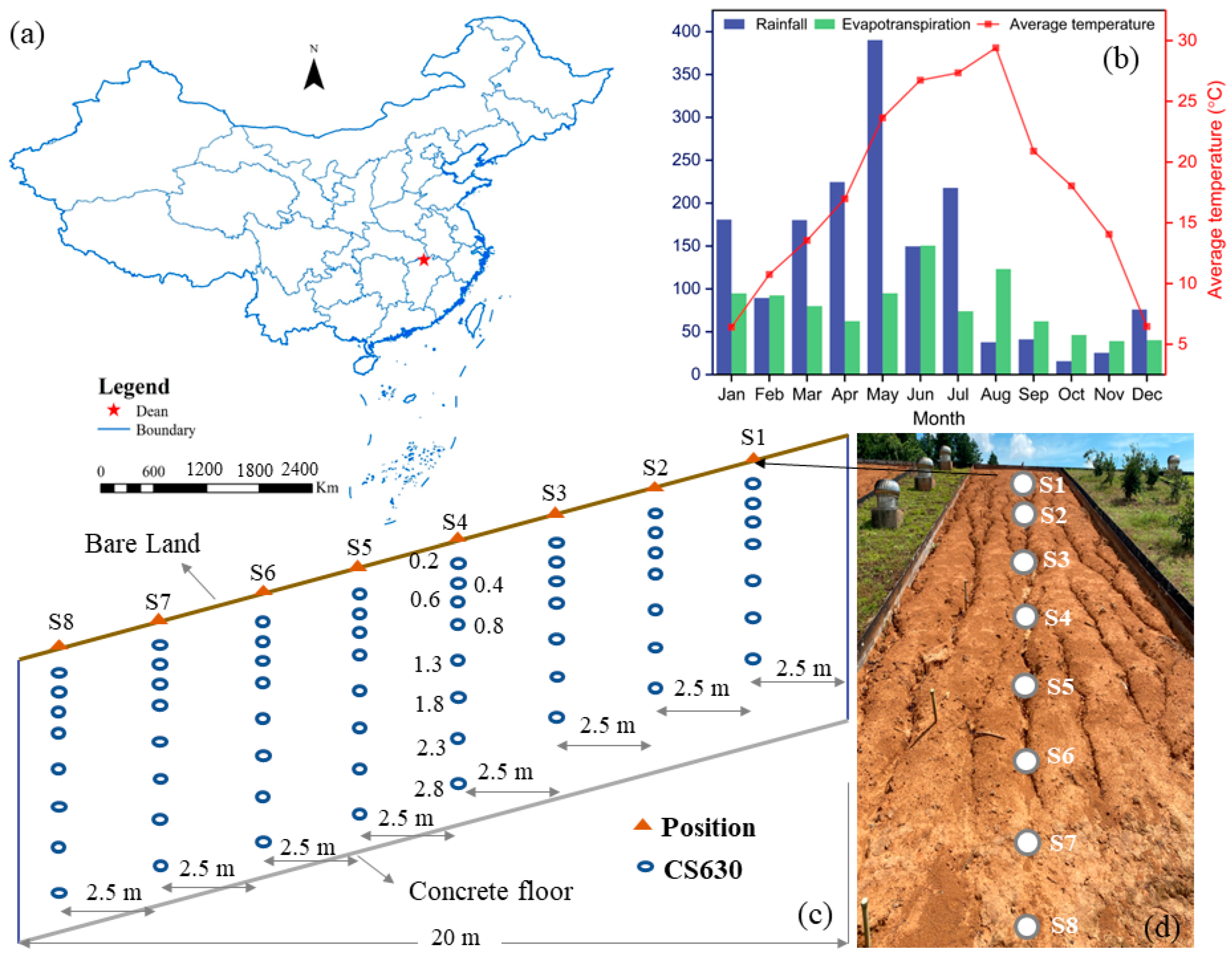
2.1. Overview of the Study Area

The study area is located in the Yangou Small watershed in Dean County, northern Jiangxi Province, on the west bank of the Boyang River of Poyang Lake, China (Figure 1a). The study area’s geographical coordinates are between 115°42′38″–115°43′06″ E and 29°16′37″–29°17′40″ N. This region experiences a continental monsoon climate with distinct seasons. The mean annual temperature in the region is 16.7 °C. It receives an annual average of 1650–2100 h of sunshine and has a frost-free period lasting between 245 and 260 days. The mean annual precipitation is approximately 1350.9 mm, with an uneven seasonal distribution resulting in a well-defined dry and wet seasons.

The total area of the study region is 80 hectares. The study region falls with the subtropical monsoon climate zone, renowned for its mild climate, pronounced seasons, ample rainfall, and simultaneous occurrence of heat and rain. The primary rainfall period in this area spans from March to June (Figure 1b). The maximum annual rainfall is 1807.7 mm, whereas the minimum is 865.6 mm. The experimental site is situated in central China’s red soil region, specifically in the southern red soil area that is classified as a second-class soil erosion region. The landform of the area is characterized as shallow and hilly, with elevations ranging from 30 to 100 m and slopes ranging from 5° to 25°. The predominant parent material of the soil are quaternary laterite and argillaceous rock. It is a typical representative of the red soil hilly region of Jiangxi Province and southern China. The geological strata include argillaceous rocks from the Proterozoic Banxi Group, quaternary red clays of the Cenozoic era, and alluvial and residual materials.

2.2. Soil Water Content Monitoring

The slope area is a runoff plot with a width of 5 m and a horizontal projection of 20 m. The bare soil has a slope of 17° (Figure 1c), with the bottom concrete plate supporting the soil being located parallel to the soil slope. The soil in the slope area was divided into four depths: A (0–0.3 m), B (0.3–0.6 m), C (0.6–1.5 m), and D (1.5 m to the bottom). The soil bulk density for each depth zone is as follows: 1.33 g·cm⁻³ for depth A, 1.47 g·cm⁻³ for depth B, 1.53 g·cm⁻³ for depth C, and 1.64 g·cm⁻³ for depth D. The slope was further divided into eight slope positions from the top to the foot of the slope. The horizontal projection of slope position S1 was 2.5 m from the top, and the horizontal distance between the two adjacent slope positions was also 2.5 m, with a total of eight slope positions (S1–S8). For each slope position, θ sensors were buried at seven or eight depths. In slope positions S1 to S3, the depths of the sensors were 0.2, 0.4, 0.6, 0.8, 1.3, and 2.7 m; from S4 to S8, an additional depth of 2.8 m (D8) was added. The θ monitoring using CS630 (Campbell Scientific, Inc., Logan, UT, USA) began in 2018, and the θ data were collected every 20 min using CR1000 data loggers (Campbell Scientific, Inc., Logan, UT, USA). For the analysis in this study, the θ data selected cover the period ranging from 1 March 2020 to 28 February 2021. However, it should be noted that the CS630 sensor located at the 0.2 m soil depth in slope position S7 may not have been in good contact with the soil, leading to inaccurate θ monitoring. Consequently, these data were excluded from the analysis.

2.3. Hydrometeorological Data

In this study, automatic weather stations were employed to monitor precipitation and air temperature. Pan evaporation was calculated by measuring the water level change in the pan. Surface runoff was determined by assessing the wall gauge reading of the surface runoff pool.

2.4. Data and Statistical Analysis

In this research, the relative deviation of θ (RD) is used to quantify the temporal stability (TS) of θ, following the approach proposed by Van Pelt and Wierenga [28]. The RD is defined as:

$${RD}_{ij}=\frac{{\theta }_{ij}-\overline{{\theta }_j}}{\overline{{\theta }_j}}$$

(1)

where θ_ij represents the θ at position i and matching time point j, and $\overline{{\theta }_j}$ is the average θ at time point j. The average θ at time point j is computed as

$$\overline{{\theta }_j}=\frac{1}{N}{\sum }_{i=1}^N{\theta }_{ij}$$

(2)

Here, N denotes the number of sample points in the research area at time point j. RD_ij represents the difference between the θ at location i and the average θ at time j. For an RD_ij time series, the average relative deviation (MRD) of θ at position i is defined as:

$${MRD}_i=\frac{1}{m}{\sum }_{j=1}^m{RD}_{ij}$$

(3)

where m is the number of observations at position i over time. The MRD quantifies the relative θ in a certain observation period with the average θ serving as the reference. Therefore, the position with an MRD value that is close to zero can be used as a representative location (RL) for monitoring θ. In this paper, 72 RD values that were calculated every day were averaged to obtain the daily MRD, which was termed as day-MRD. The standard deviation of RD (SDRD) can be expressed as:

$${SDRD}_i={\left[\frac{1}{m-1}{\sum }_{j=1}^m{\left({RD}_{ij}-{MRD}_i\right)}^2\right]}^{0.5}$$

(4)

SDRD describes the time variability of RD and is also an important index value to measure the TS. The smaller the value of SDRD, the higher the TS [29].

A relative deviation analysis of θ was used to judge the mean difference between any observation point and the study area. If the observation value of a sample point was close to the average value of the study area every time, it was considered as an RL. To accurately determine the RL, different scholars have chosen different methods. Vachaud et al. [15] used the point with the MRD close to zero as the RL, but MRD was a statistical indicator and shifted within the range of SDRD. When MRD approaches zero, its matching SDRD is not necessarily minimal. Guber et al. [30] selected the point with the minimum MRD and SDRD as the RL. Therefore, it may be impossible to choose accurate RLs based on MRD or SDRD alone. Jacobs et al. [31] regarded MDR and SDRD as the two right angles of a triangle and used the hypotenuse length as the index of TS (ITS):

$${ITS}_i=\sqrt{{MRD}_i^2+{SDRD}_j^2}$$

(5)

The smaller the ITS value is, the stronger the TS is.

In this paper, MRD had a good consistency with ITS, so MRD was selected as the index of the TS analysis. The MRD calculation in this paper was based on two data sets, one of which was obtained via the all-time series data calculation (referred to as all-MRD), and the other was obtained by performing a data calculation of every day (referred to as day-MRD). MRD in the range of [−5%, 5%] is considered the time stable of θ [31].

The root mean square error (RMSE) was used to evaluate the prediction accuracy of θ in the representative samples. RMSE effectively reflects the accuracy of the predictions, with smaller values indicating higher accuracy. The calculation formula for RMSE is defined as:

$$RMSE=\sqrt{\frac{{\sum }_{i=1}^n{\left(X_{obs,i}-X_{pre,i}\right)}^2}{n}}$$

(6)

where n is the number of observations, X_obs,i represents the ith observed value, and X_pre,i represents the ith predicted value.

3. Result

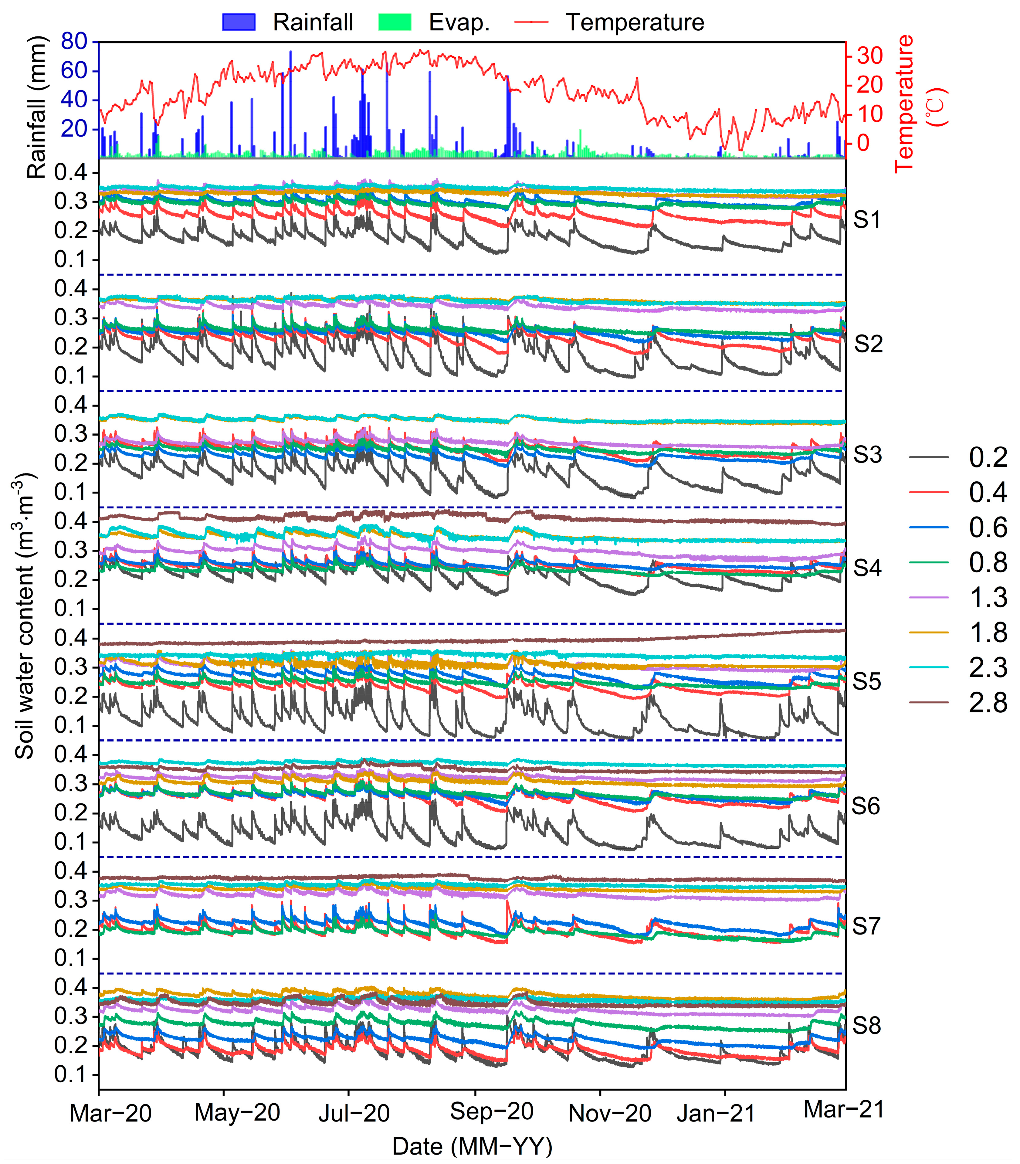
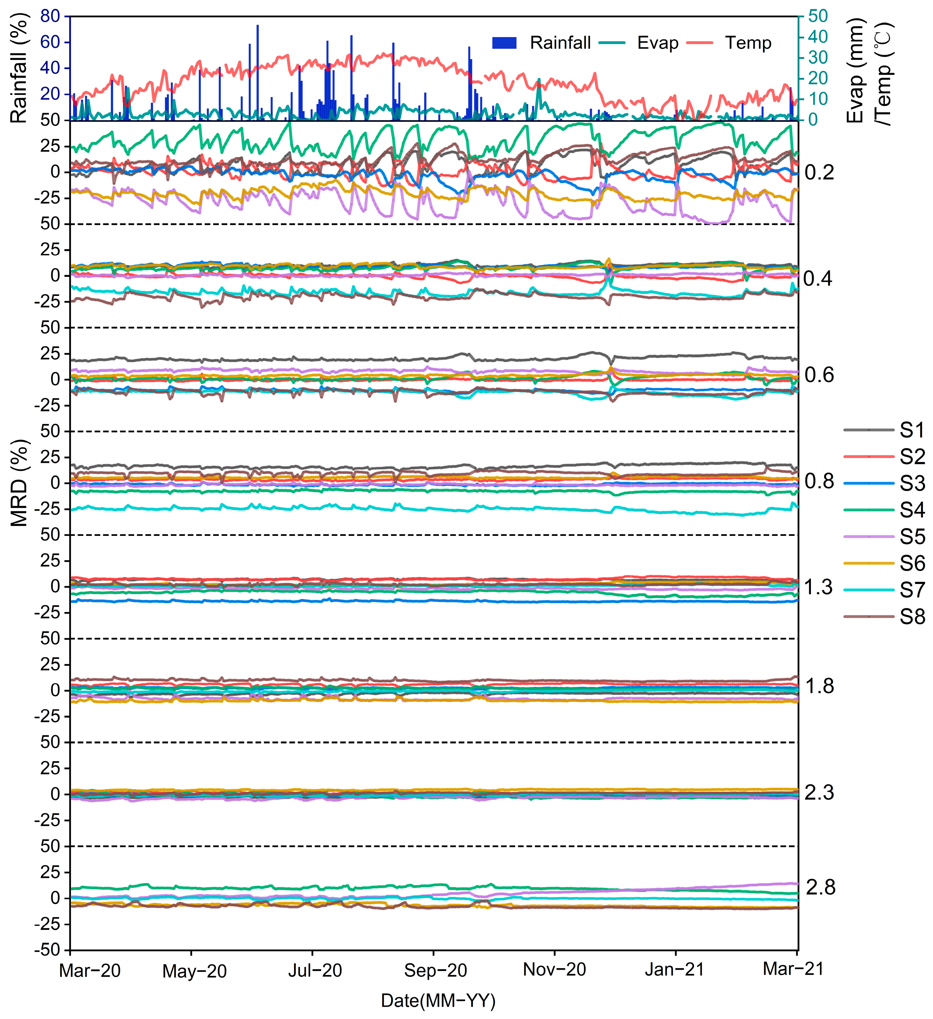
3.1. Soil Water Content Dynamics

As shown in Figure 2, the θ at different soil depths within each slope had a similar trend of change, displaying a response to rainfall that gradually weakened with the increase in soil depth. The rainy season maintained the θ at a high level, with notable instances of heavy rainfall occurring on 7 July, 9 August, and 16 September, which resulted in several prominent θ peaks. Among the soil depths, the θ at the 0.2 m depth exhibited the most pronounced response to rainfall, displaying the largest temporal variability. Below depths of 0.8 m, the θ displayed a weaker response to rainfall. This can be attributed to two reasons. Firstly, rainfall requires time to infiltrate deeper into the soil. Additionally, the θ of the deeper soil layers tends to be higher, leading to the formation of preferential flow paths as the rainfall infiltrates the deep soil. The fluctuation frequency of θ was also correlated with the seasons, with a higher swing frequency observed in spring and summer, when rainfall is more frequent. Conversely, autumn and winter are characterized by lower rainfall frequencies and exhibited a lower fluctuation frequency of θ. Following late October, θ displayed the lowest fluctuation frequency due to reduced rainfall and an extended dry–wet cycle that was facilitated by evaporation.

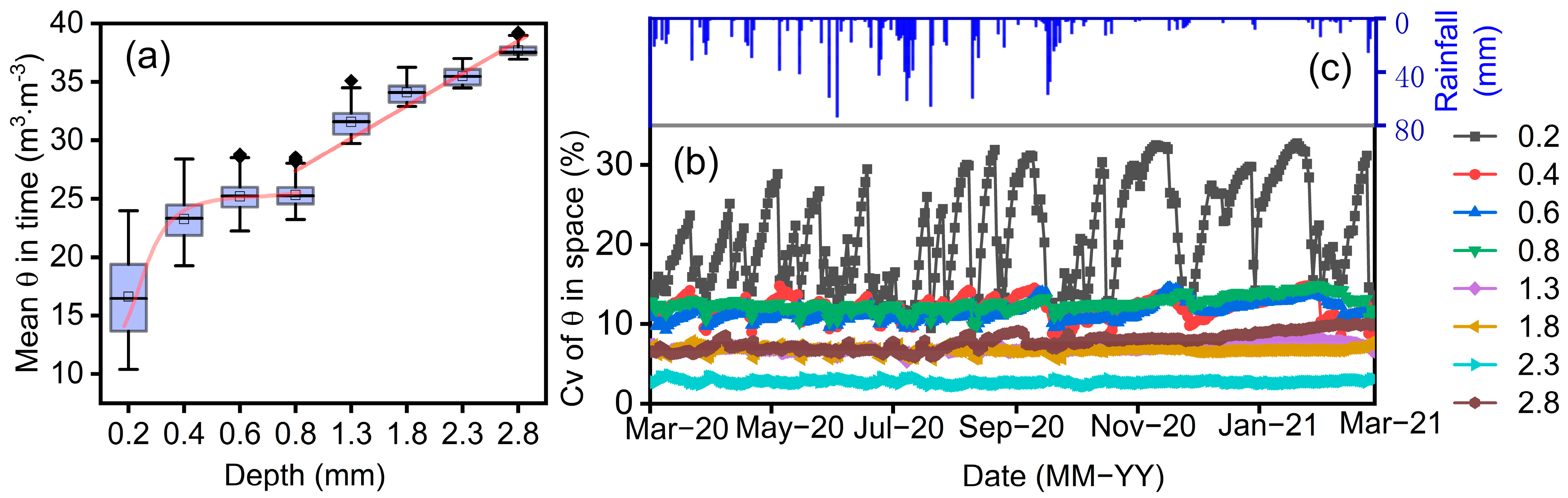
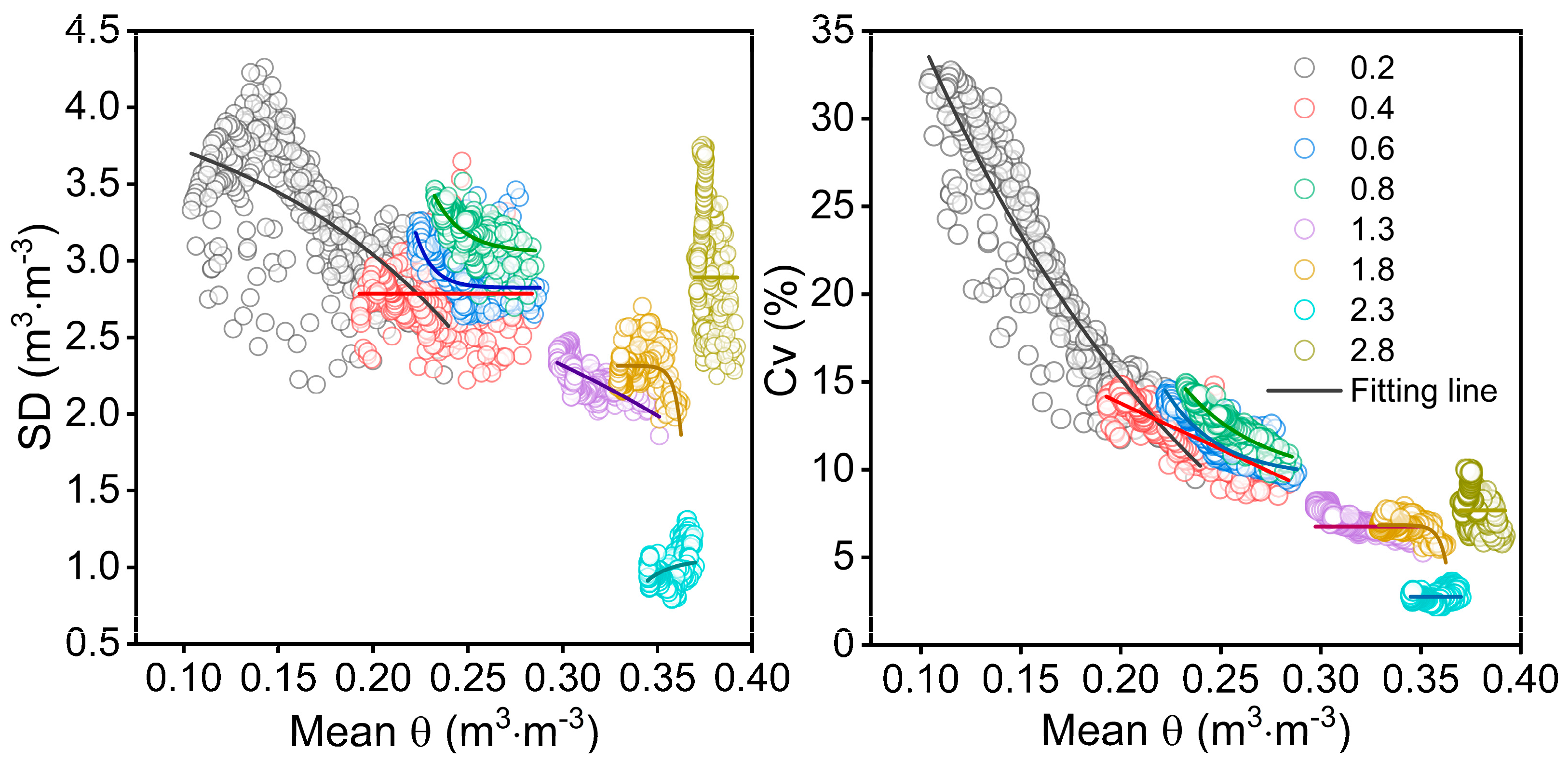
3.2. Descriptive Statistics of Soil Water Content

The mean water content over the all-time series (${\overline{\theta }}_t$) exhibited an increasing trend with the soil depth across different slope positions. In addition, the range and coefficient of variation (C_v) decreased with the increase in soil depth, indicating that water replenishment through infiltration or macropore flow enhanced the time stability of θ at greater soil depths (

Table 1. Descriptive statistics of θ in different soil depths at each slope position in time.

Position	0.2 m		0.4 m		0.6 m		0.8 m		1.3 m		1.8 m		2.3 m		2.8 m
	Mean	Cv	Mean	Cv	Mean	Cv	Mean	Cv	Mean	Cv	Mean	Cv	Mean	Cv	Mean	Cv
S1	0.17	15.8	0.25	8.1	0.3	4.8	0.29	3.4	0.34	3.8	0.33	1.9	0.35	1.8	-	-
S2	0.17	27.5	0.23	11	0.25	6.1	0.26	4.3	0.34	3	0.36	2	0.36	2.5	-	-
S3	0.16	24.4	0.25	8.7	0.23	6.9	0.25	4.5	0.27	4.1	0.35	2.2	0.35	2.1	-	-
S4	0.21	15.1	0.25	7.1	0.26	4.2	0.23	5.1	0.3	5.4	0.35	3.1	0.35	4.4	0.41	2.6
S5	0.12	36.1	0.23	8.3	0.27	6.6	0.25	4.8	0.31	4.4	0.31	3.5	0.34	1.7	0.4	3.4
S6	0.13	27.3	0.25	8.5	0.26	5.2	0.27	4.4	0.32	2.6	0.31	3.3	0.37	1.7	0.35	2.4
S7	-	-	0.19	11.4	0.22	8.2	0.19	7.4	0.32	3.4	0.34	1.9	0.35	1.5	0.38	1.3
S8	0.18	18.4	0.19	10.8	0.22	7.2	0.28	5	0.32	3.8	0.38	2.9	0.36	1.7	0.35	2.9

Notes: Mean is the mean of θ; C_v is the coefficient of variation of θ.

). At a soil depth of 0.2 m, the ${\overline{\theta }}_t$ in slope position S5 was the lowest (0.12 m³·m⁻³), while S4 recorded the highest value (0.21 m³·m⁻³). At a soil depth of 2.8 m, slope S8 displayed the lowest value (0.35 m³·m⁻³), while S4 was the highest (0.41 m³·m⁻³). The average of ${\overline{\theta }}_t$ for each soil depth indicated that S4 had the highest water retention (0.30 m³·m⁻³), whereas S5 had the lowest (0.28 m³·m⁻³), suggesting that there was better water retention in S4. The C_v of θ at the 0.2 m soil depth ranged from 15.1% to 36.1%, indicating strong temporal variability in the surface soil. For other soil depths, the C_v was less than or close to 10%, indicating weak temporal variability. Thus, it can be concluded that the surface soil experienced the most significant temporal variability in θ. Notably, slope S7 exhibited the lowest average C_v across different soil depths (5.01%), indicating an overall good stability of θ in slope S7. The mean θ in space (${\overline{\theta }}_s$) increased with depth with an exponential relationship above 1.3 m (initial increase followed by stabilization). Below 1.3 m, ${\overline{\theta }}_s$ linearly increased (Figure 3a). The 0.2 m soil depth displayed strong spatial variability in ${\overline{\theta }}_s$ due to external factors such as rainfall, evaporation, soil erosion, air temperature, and wind, which caused disturbances. The C_v decreased with rainfall, suggesting that rainfall contributed to more uniformity in the spatial distribution of θ. At soil depths of 0.4 m to 0.8 m, the C_v of θ ranged around 10%, indicating moderate spatial variability. Below 1.3 m, the C_v was less than 10%, indicating weak spatial variability (Figure 3b).

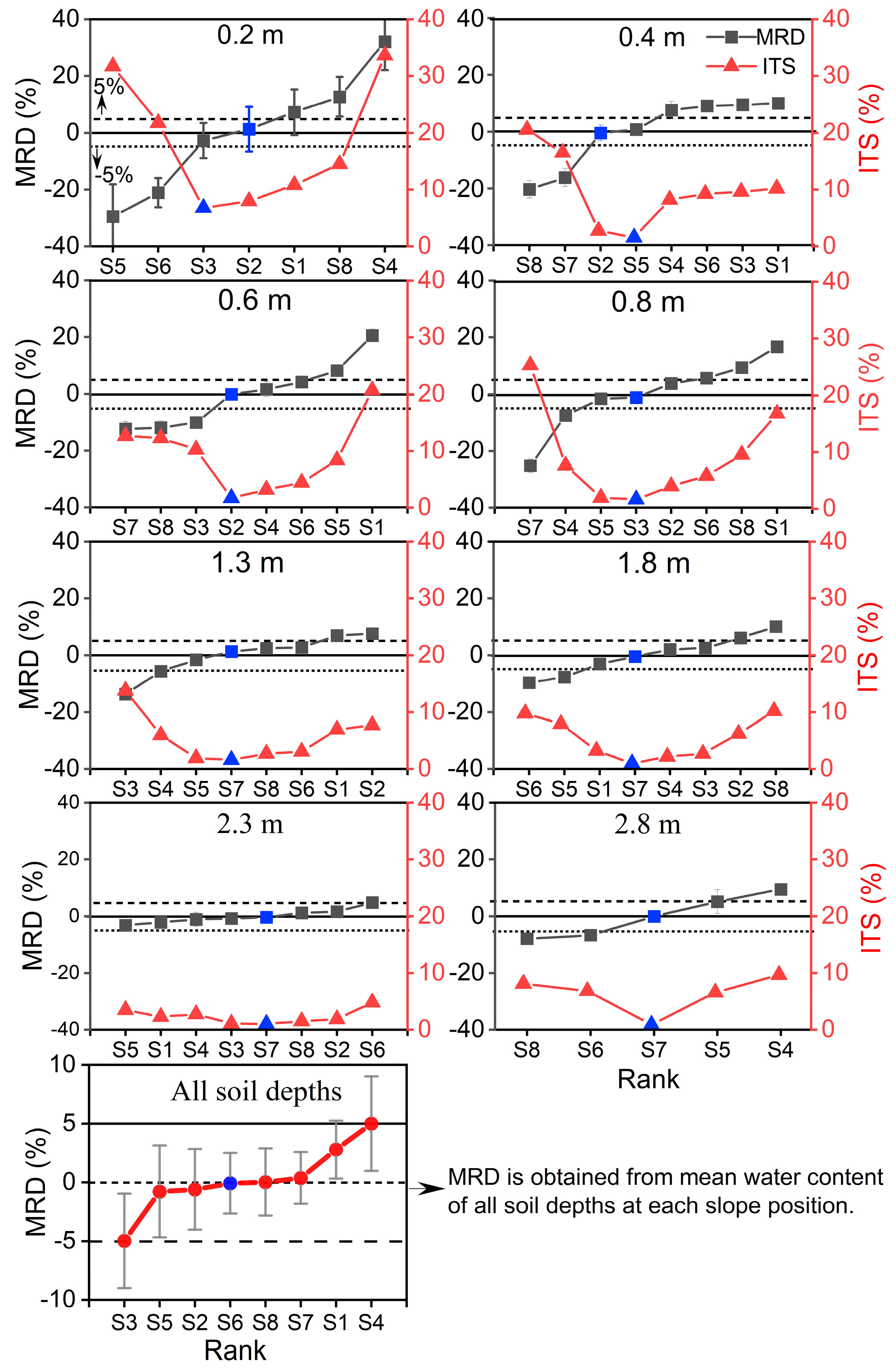
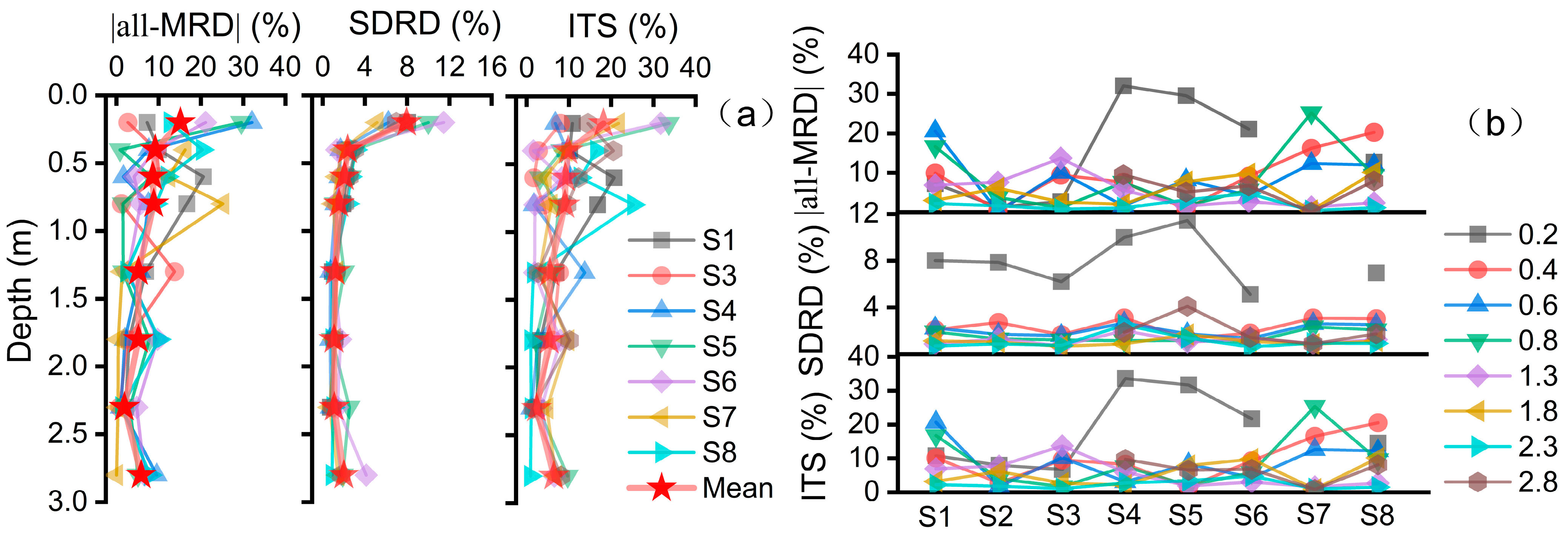
3.3. Temporal Stability of Soil Water Content

Figure 4 shows the ordering diagram of the MRD of θ at different soil depths for each observation point along the slope, which have been arranged in ascending order. The error bar corresponds to the SDRD. The MRD values at the 0.2, 0.4, 0.6, 0.8, 1.3, 1.8, 2.3, and 2.8 m soil depths were 61.7%, 26.19%, 32.56%, 24.24%, 13.22%, 17.86%, 6.94%, and 17.44%, respectively. The SDRD values at the same soil depths were 6.31%, 1.77%, 1.31%, 1.08%, 1.12%, 0.97%, 1.88%, and 3.21%, respectively. Correspondingly, the ITS values were 61.98%, 10.17%, 20.69%, 16.78%, 7.73%, 10.17%, 4.82%, and 17.73%, respectively. At the 0.2, 0.4, 0.6, 0.8, 1.3, 1.8, 2.3, and 2.8 m soil depths, the MRD values close to zero were observed at slope positions S2, S2, S2, S3, S7, S7, S7, and S7, respectively. These findings indicate that the stable locations vary across different soil depths, and no single location can fully represent the θ characteristics of the entire soil profile [32].

3.4. TS Diurnal Variation of Soil Water Content

The variation in the diurnal MRD (day-MRD) exhibited significant variation across different soil depths and demonstrated a correlation with the response of day-MRD to rainfall at the 0.2 m soil depth (Figure 5). Furthermore, rainfall reduced the absolute value of day-MRD, bringing it closer to zero, thereby suggesting that rainfall can enhance the TS of θ. The variation range in day-MRD notably differed across various soil depths, particularly at the 0.2 m soil depth. For each slope position at the 0.2, 0.4, 0.6, 0.8, 1.3, 1.8, 2.3, and 2.8 m soil depths, the day-MRD ranged between 24.8% and 50.8%, 6.0% and 21.3%, 8.2% and 13.7%, 4.3% and 14.4%, 3.6% and 7.1%, 2.9% and 9.6%, 2.2% and 9.2%, and 4.4% and 14.9%, respectively. This indicates that the degree of variation decreased with increasing depth. The C_v of day-MRD values for different soil depths in each slope position exceeded 10%, indicating substantial temporal variation in day-MRD, with the 0.2 m soil depth displaying the most pronounced variation. These findings underscore that day-MRD exhibits notable temporal variation and caution against selecting representative samples based on short time intervals or lower frequency monitoring data, especially for the soil depths of 0.2, 0.4, and 0.6 m, as it could introduce a higher probability of errors in the estimation of the mean value of θ.

This study examined the proportions of RL (representative location) days based on day-MRD values that are less than 5% across different soil depths for 365 days (Figure 6). The analysis revealed no significant consistency between the daily proportions of RL and soil depth at individual sampling points. For instance, at sample site S1, the soil depths of 0.2, 0.6, 1.3, and 2.3 m accounted for 45.30%, 0%, 1.10%, and 100% of the daily proportions of RL, respectively; for position S4, the soil depths of 0.2, 0.6, 1.3, and 2.3 m accounted for 0%, 85.91%, 57.46%, and 100%, respectively. These findings indicate that the TS of θ, as assessed by day-MRD, is not influenced by soil depth. Furthermore, no significant relationship was observed between day-MRD and slope position. The daily proportions of RL for positions S1, S3, S5, and S7 at the 0.4 m soil depth were 83%, 55%, 100%, and 55%, respectively. At the 1.8 m depth, positions S1, S3, S5, and S7 accounted for 94.20%, 100%, 6.08%, and 100% of the daily proportions of RL, respectively. These results further confirm that the TS of θ, as assessed by the day-MDR analysis, is not affected by slope position. In summary, the proportion of RL days at the 0.2 m soil depth was the smallest, demonstrating the weakest TS of θ at this soil depth. Conversely, the proportion of RL days in the 2.3 m soil depth was the greatest, indicating the highest TS of θ at this depth.

4. Discussion

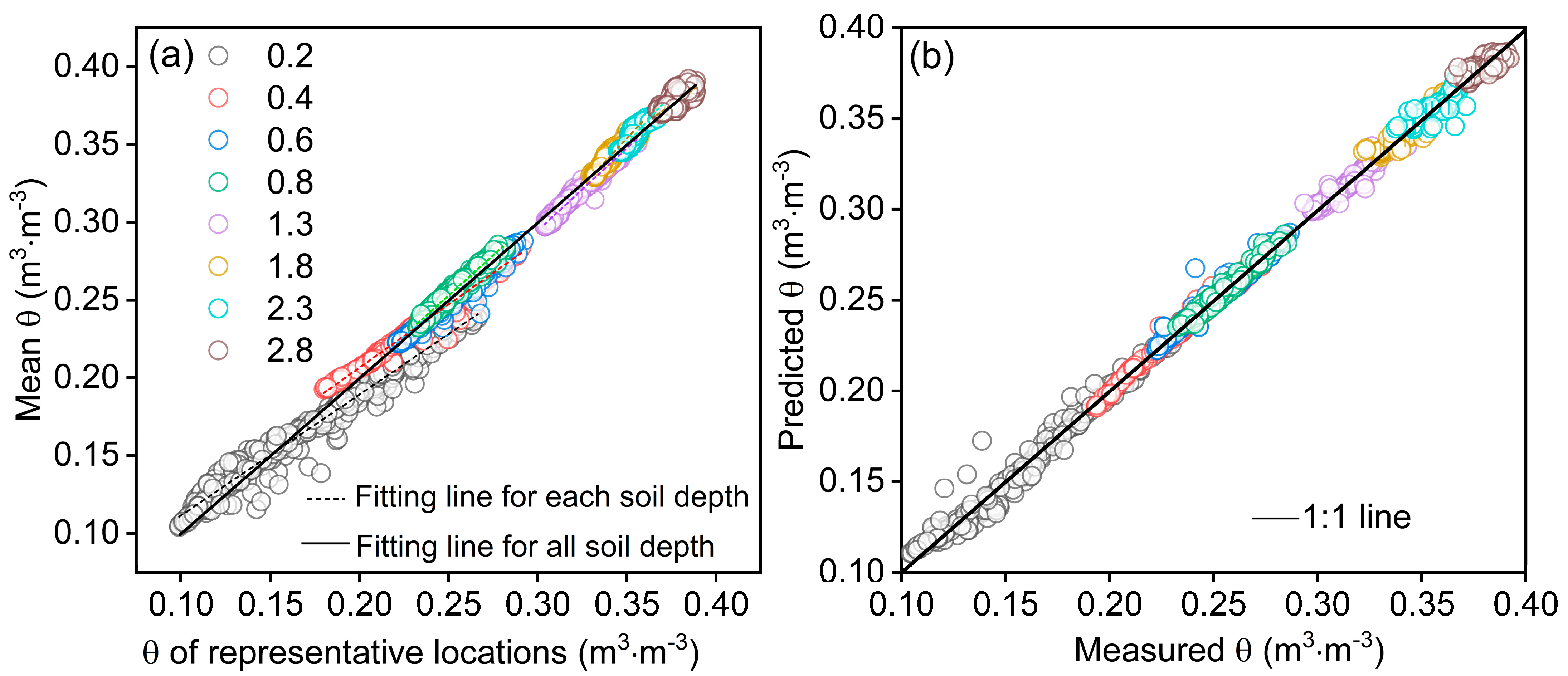
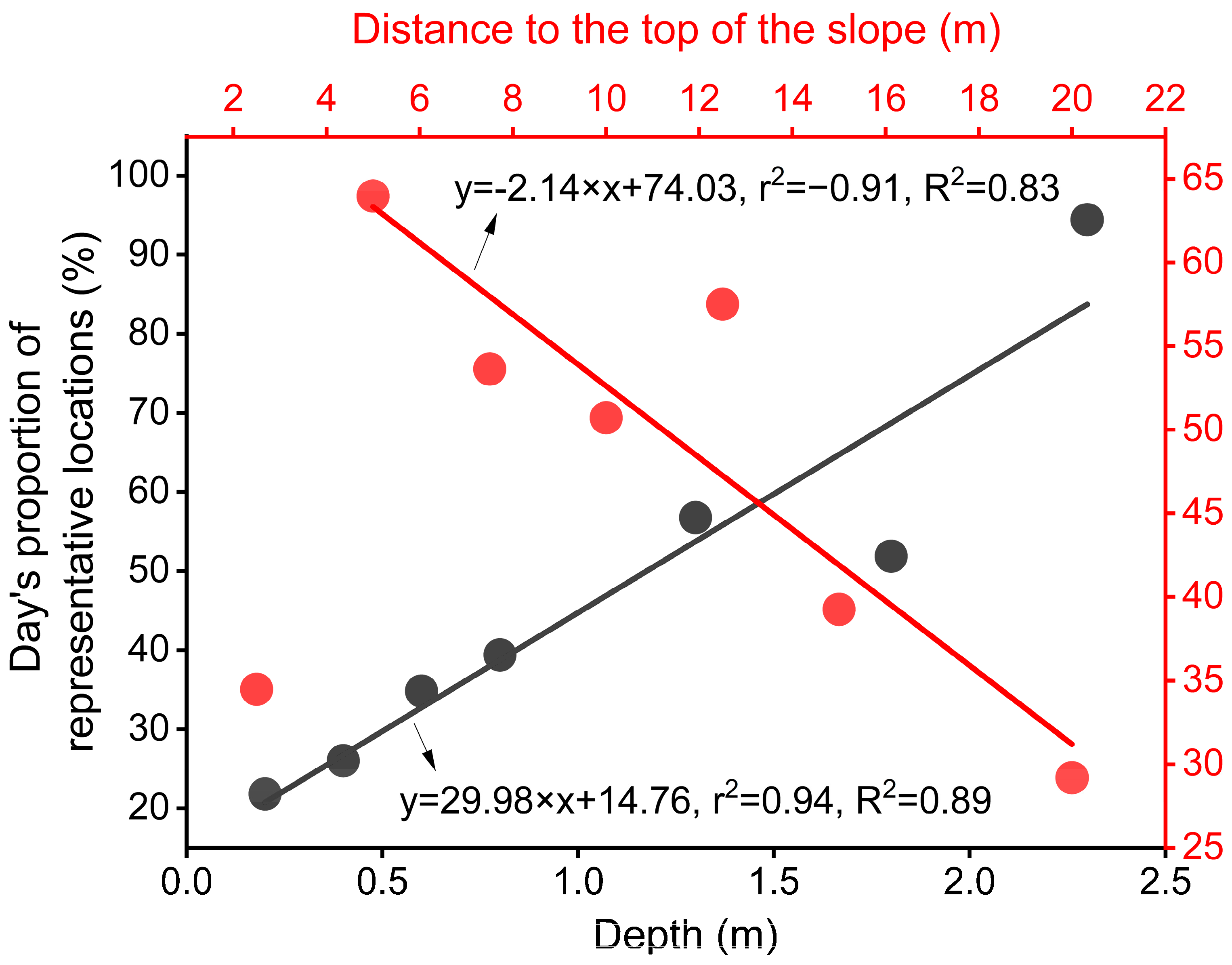
4.1. Soil Water Content Predicted by Representative Locations

In this study, representative θ samples were selected at different soil depths using the MRD discrimination method. A linear regression analysis was conducted between the mean θ and the θ values in the representative samples (Figure 7). With the exception of the soil depths of 2.3 and 2.8 m, the coefficients of determination for the regression prediction models at other soil depths exceeded 0.9. A lower RMSE value indicates a smaller difference between the predicted and observed values, which reflects higher prediction accuracy. The regression model successfully estimated the mean θ, as evident from the observed and predicted values aligning along the 1:1 line scatter points. Among the soil depths, the 0.2 m depth exhibited the largest RMSE (0.6%), whereas the 1.3 m soil depth had the smallest RMSE (0.17%). Overall, the prediction errors of representative samples for the mean θ at each soil depth were all below 1%, and the prediction results were considered accurate when the RMSE was less than 2% [33]. The findings demonstrate that the mean θ on sloping land can be accurately predicted based on representative samples of θ. Moreover, the prediction accuracy of θ in this study was slightly higher than that reported in previous studies [12,24,34], which can be attributed to the high-frequency θ monitoring method used in this study.

4.2. Spatial Distribution Characteristics of Soil Water Content on the Slope

The spatial distribution pattern of θ is influenced by both soil depth and slope position, as depicted in Figure 8. The mean θ at each slope position demonstrates an increasing trend with soil depth. Specifically, the mean θ at positions S4 and S8 exhibited a linear relationship with soil depth, while the mean θ at other slope positions followed an exponential relationship. Because the study area is bare land, there is no water absorption by the deep roots. Consequently, θ migrates downwards and gradually accumulates at greater depths [35]. The C_v of θ in each slope position showed an exponential decline with increasing soil depth. Beyond a soil depth of 0.8 m, the C_v became less sensitive to variations in soil depth. These findings indicated that while θ increases with increasing soil depth, the spatial variability of θ decreases. Except for the 2.3 and 2.8 m soil depths, the other depths exhibited a linear decrease with the distance from the slope top, whereas the remaining other soil depths displayed a linear increase. Previous research by Gao et al. [23] reported a significant negative correlation between θ and the seaward slope, with a greater influence of the seaward slope being observed at greater soil depths. The complex nature of soil erosion in the study area, which may be situated in a closed area, contributed to the intricate relationship between θ and altitude. Moreover, apart from the 2.3 and 2.8 m soil depths, the C_v showed a linear decrease with distance from the slope top, while the other soil depths exhibited a linear increase. These observations suggest that the spatial variability of θ was greater uphill compared with downhill.

The relationship between the standard deviation (SD) of the C_v and water status provides insights into the heterogeneity of the spatial variation of θ [25]. The SD exhibited a decreasing trend with the mean θ (p > 0.05), and the relationship varied among different soil depths (Figure 9). Conversely, a significant decreasing exponential relationship was observed between the C_v and the mean θ (p < 0.05). This finding aligned with the observations made by Pan and Peters-Lidard [36], who reported that SD decreased with θ surpassed a threshold, while SD increased when θ fell below the threshold. The current study identified a threshold of 0.35 m³·m⁻³ on the sloping land, indicating that SD and θ exhibited an increasing relationship when θ exceeded the threshold. Apart from the soil depths of 2.3 and 2.8 m, the relationship between the C_v and mean θ demonstrated consistency. This behavior indicated a reduced variability of θ under increasingly wet conditions, which was consistent with the findings from previous studies [37,38]. The results further support the notion that θ distribution on the slope increased even as θ increased.

4.3. Temporal Stability Characteristics of Soil Water Content on Slope

Compared with the results from previous studies [27], the present study reveals a significantly higher MDR. Given that the study area consists of a bare soil slope, soil erosion greatly influences it. However, compared with other studies [12,19,24,25,39], our findings indicate a smaller MDR. The presence of vegetation often hampers the maintenance of similar spatial patterns [40,41,42]. Because the study area is predominantly bare land, the TS of θ is higher than in areas covered by vegetation. It is important to note that direct comparisons among different studies may be challenging due to variations in the landscapes, land uses, sampling schemes, and monitoring periods [43]. Interestingly, the maximum TS of θ on the slope was not observed at the center but rather at the upper and lower slope positions. Except for slope position, the minimum MRD of the 0.2 and 0.4 m soil depths slightly differed from the ITS, while the minimum values of other soil depths matched the same slope positions. This suggested that both MRD and ITS could be used to identify the representative sample of θ at specific locations. In our study, the average θ of different soil depths at each slope position served as the sampling point, and the results indicated that slope position S6 was the most representative sample point. This further underscored that the representative sample point did not necessarily lie at the center of the plot.

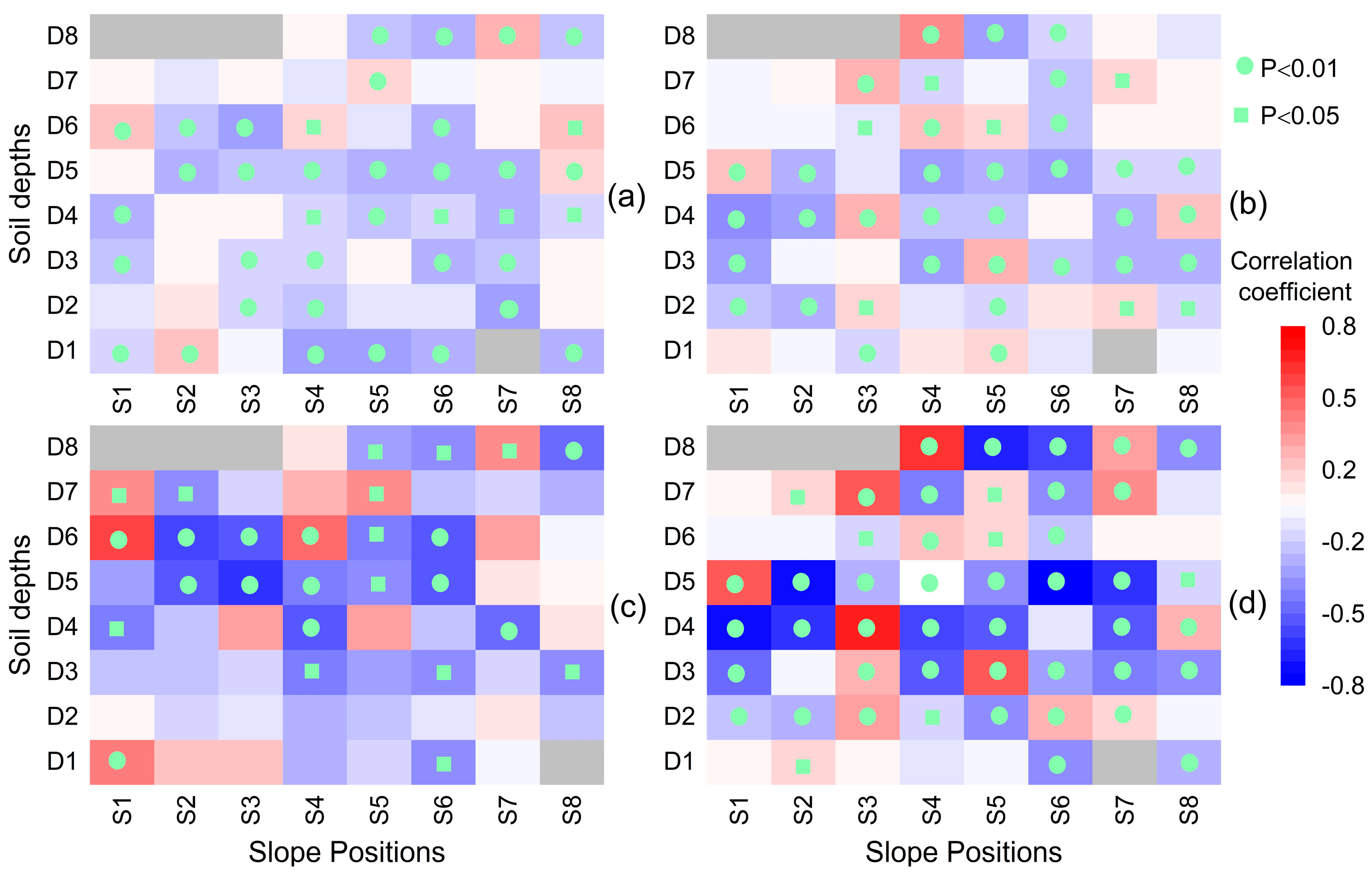
4.4. Effects of Depth and Slope Position on the Temporal Stability of Soil Water Content

The analysis of |all-MRD| (absolute value of all-MRD) and ITS of different slope positions revealed significant variations and inconsistencies with soil depth (Figure 10a). These findings suggest that the TS of θ, as indicated by |all-MRD| and ITS, did not exhibit a consistent depth dependence for a certain slope position. The distribution of |all-MRD| and ITS greatly differed among different slope positions, which can be attributed to soil heterogeneity and variations in preferential flow processes. However, when averaging the |all-MRD| and ITS values across all soil depths, a clear pattern emerged: both measures decreased with increasing depth, which indicated a depth-dependent TS of θ for the entire slope plot. Notably, |all-MRD| at soil depths above 1.3 m was significantly higher than at the depths below it, indicating that θ in the soil depths below 1.3 m had better TS. However, SDRD exponentially decreased with soil depth in each slope position. Consistent with previous research by Gao et al. [23], SDRD demonstrated an exponential decrease with soil depth in each slope position. Moreover, the results indicated minimal differences in SDRD among different soil depths, while the variation of θ deviation from the mean value decreased with the increase in soil depth for each slope position. When examining the relationship with the distance from the top of the slope (Figure 10b), both |all-MRD| and ITS displayed variations. Particularly, |all-MRD| and ITS at a soil depth of 0.2 m were significantly higher than corresponding values in other soil depths in the middle of the slope, indicating a weak TS of θ at this soil depth. These findings align with the research results of Gao et al. [27].

Our findings aligned with a previous study by Takagi and Lin [44], which demonstrated that the subsurface (ranging from 0.3 to 1.1 m) exhibited increasing TS with depth. However, in the soil interval of D5–D8 (1.3–2.8 m), |all-MRD| showed a linear increase with the θ. A subsurface lateral flow below 1.3 m likely weakened the TS of θ. These observations support earlier studies [44,45] and highlight the significance of subsurface lateral flow in influencing θ dynamics at intermediate depths. Consequently, it can be concluded that the TS of θ increased with depth in soil depths of less than 1.3 m, while it decreased with increasing depth in soil depths that were greater than 1.3 m. This indicated that θ at the 0.2 m soil depth exhibited the weakest TS, consistent with a previous study [46], whereas the 1.3 m soil depth exhibited the highest TS.

As discussed in Section 3.4, the depth and slope position did not have a significant effect on the TS of θ based on day-MRD. However, when considering all slope site samples, we observed a significant linear increase in the proportion of representative days with soil depth (R² = 0.89). This indicated that the TS of θ at the plot scale is influenced by soil depth, increasing with the increase in depth (Figure 11). This finding is consistent with a previous study [12]. However, our results differ from those reported by Xu et al. [34], who suggested that the surface depth exhibited the highest TS; we found that the 0.2 m depth exhibited the weakest TS. Several factors may account for these discrepancies. Firstly, Xu et al. [34] conducted their study in an arid region where the impact of rainfall is less pronounced compared with our region. Secondly, the plots studied by Xu et al. [34] were flat terraced fields, whereas our study featured a 17° slope with no vegetation coverage, leading to weaker TS in the surface soil due to soil erosion. More importantly, Xu et al.’s research relied on the artificial monitoring of θ, which has a lower measurement frequency and may miss the most unstable θ information at any given moment. Our results also differed from Zhu et al. [47], who reported no depth effect on the TS of θ due to the influence of roots and gravel. For the 0.2 m soil depth, the proportion of representative days across all slope positions was 34.49%. The surface soil was greatly influenced by rainfall, erosion, and evaporation, which led to a weaker TS. Except for the 0.2 m soil depth, the proportion of representative days exhibited a significantly linear decrease with slope length (R² = 0.83). This indicates that the TS of θ at the profile scale is influenced by slope length, with a decrease in TS of θ occurring as the distance from the slope top increases. These findings differ slightly from those of Zhao et al. [39], who reported that the topography had a weak influence on the TS of θ. This may have been because the measured surface θ (0–6 cm) did not capture the possible topographical impacts at greater depths. In humid environments, water redistribution is likely dominated by both vertical and slope direction fluxes most of the time. Therefore, soil depth and slope position significantly influence the TS of θ. In conclusion, the influence of depth and slope position on the TS of θ based on day-MRD differed from that which was based on all-MRD. Consequently, using the MRD over a long time series to assess the TS of θ at a specific location may lead to significant deviations. The temporal variability of MRD can be better analyzed by examining the variation of day-MRD, which provides a more accurate assessment of the TS of θ.

4.5. Effects of Air Temperature and Hydrometeorological Conditions on the Temporal Stability of Soil Water Content

Rainfall played a significant role in influencing day-MDR as it is strongly correlated with rainfall, evaporation, air temperature, and surface runoff (Figure 12). This indicated that the TS of θ was influenced by meteorological and hydrological conditions, which had different effects at different slope positions and soil depths. Notably, there was a negative correlation between rainfall and day-MDR, indicating that rainfall improved the TS of θ. Consequently, θ exhibits greater stability during the rainy season. This finding aligns with previous research by Zhao et al. [39], which also suggested that the spatial patterns of θ became more stable over time during wet seasons but less stable during dry or transitional periods. In semi-arid steppe regions, rainfall drives the system towards equilibrium, enhancing its TS of θ. It is worth noting that the correlation coefficient between day-MDR and rainfall was the highest for the surface soil, indicating that rainfall had the greatest impact on surface soil due to direct replenishment. However, the influence of rain on day-MRD was relatively minor at the 2.3 m depth, as deeper soil layers were more likely to be influenced by subsurface flow processes [27].

Evaporation and runoff have noticeable effects on the TS of θ. The day-MDR of most soil depths exhibited a significant negative correlation with evaporation across all slope positions. This suggests that soil evaporation contributes to improving the TS of θ. It is worth noting that evaporation mainly occurred above the 0.2 m soil depth [48,49]. However, the greatest influence of evaporation on day-MDR was observed at the soil depth of 0.8 m, contrary to expectations. Runoff refers to water movement at the soil surface following rainfall [50]. For the 0.2 m soil depth, runoff at slope position S1 exhibited a significantly positive correlation with day-MDR, whereas runoff at slope position S6 demonstrated a significantly negative correlation. These findings indicate that runoff decreased the TS of θ at slope position S1 while it improved the TS at slope position S6. This behavior can be attributed to the complex nature of the underlying surface conditions on the slope. As shown in Figure 1, the presence of gullies and ravines with spatiotemporal heterogeneity increased the effects of runoff on the TS of θ. It is important to note that, similar to evaporation, the influence of runoff on day-MDR was not strongest at the 0.2 m soil depth. Instead, it exerted the greatest impact on the 1.8–2.3 m soil depth. This phenomenon may be attributed to the combined effects of surface runoff and internal water flow in deep soil. Thus, surface runoff can potentially enhance the TS of deep soil water. Overall, both evaporation and runoff play significant roles in shaping the TS of θ. Evaporation contributes to an improved TS, especially at the 0.8 m soil depth, while runoff impacts the TS differently depending on the slope position and soil depth. These findings shed light on the complex dynamics of θ and emphasize the need for comprehensive assessments of evaporation and runoff in understanding the temporal behavior of θ.

Air temperature plays a significant role in influencing the TS of θ. Surprisingly, the correlation between temperature and day-MDR was found to be stronger than that of other hydrological conditions, indicating that temperature had the most pronounced impact on the TS of θ. This finding aligns with the research conducted by Mahmood et al. [51] who discovered that the effect of maximum surface temperature on variations in θ produced much stronger cross-correlations compared with precipitation. Thus, air temperature emerges as the most influential factor affecting the TS of θ. Interestingly, the influence of air temperature on the TS of θ is not the strongest in the surface soil but at the deep soil of 1.3 m. This suggests that the impact of air temperature on the TS of θ extends beyond the surface layer and has a notable effect on deeper soil layers.

5. Conclusions

An accurate and comprehensive understanding of θ dynamics is crucial for hydrological applications. In this study, we assessed the spatial variability and temporal stability (TS) characteristics of θ on a slope using high-temporal resolution monitoring data. Our analysis involved statistical methods and TS analysis to gain insights into the frequency, degree, and influencing factors of the TS of θ based on diurnal observations over 365 days. By employing this approach, we could comprehensively evaluate the spatial variability and TS of θ on a microscale slope in the subtropical red soil region of China. Our study aimed to quantify the factors influencing the spatiotemporal variability of θ in this region.

This study provides valuable insights into the temporal and spatial variability of θ on a microscale slope. The θ showed higher spatial variability for shallow soils and wet seasons compared with deep soils and dry seasons. The results indicate that the TS of θ is higher on the upper and lower slopes than the middle slope. The diurnal variation of the TS of θ on the slope was primarily influenced by soil depth, slope position, air temperature, and hydrological conditions. Notably, the influence of soil depth on TS was greater than that of slope position, and the influence of air temperature was greater than that of hydrological conditions. It is important to note that this study was based on one year of data and presents the preliminary results from a well-controlled microscale experiment on a bare slope. Therefore, some several points and limitations should be addressed in future research. Firstly, conducting multi-year studies to assess the spatiotemporal variability characteristics of θ in different hydrological years is necessary. Additionally, although on a small-scale slope, the effect of soil texture also needs to be considered. Furthermore, future investigation into the spatiotemporal variability of θ on slopes covered by different vegetation types is warranted. The research object of this paper is bare land, so it is necessary to study it further. In conclusion, this study contributes to our understanding of the temporal and spatial variability of θ on slopes and highlights the influence of various factors. The identified limitations guide future research to advance our knowledge of θ variability in different contexts and improve prediction accuracy.

References

1. McColl, K.A.; Alemohammad, S.H.; Akbar, R.; Konings, A.G.; Yueh, S.; Entekhabi, D. The global distribution and dynamics of surface soil moisture. Nat. Geosci. 2017, 10, 100–104. [Google Scholar] [CrossRef]
2. Meng, S.; Xie, X.; Liang, S. Assimilation of soil moisture and streamflow observations to improve flood forecasting with considering runoff routing lags. J. Hydrol. 2017, 550, 568–579. [Google Scholar] [CrossRef]
3. Massari, C.; Camici, S.; Ciabatta, L.; Brocca, L. Exploiting Satellite-Based Surface Soil Moisture for Flood Forecasting in the Mediterranean Area: State Update Versus Rainfall Correction. Remote. Sens. 2018, 10, 292. [Google Scholar] [CrossRef] [Green Version]
4. Greco, R. Soil water content inverse profiling from single TDR waveforms. J. Hydrol. 2006, 317, 325–339. [Google Scholar] [CrossRef]
5. He, H.; Aogu, K.; Li, M.; Xu, J.; Sheng, W.; Jones, S.B.; González-Teruel, J.D.; Robinson, D.A.; Horton, R.; Bristow, K.; et al. A review of time domain reflectometry (TDR) applications in porous media. Adv. Agron. 2021, 168, 83–155. [Google Scholar] [CrossRef]
6. Gamage, D.N.V.; Biswas, A.; Strachan, I.B.; Adamchuk, V.I. Soil Water Measurement Using Actively Heated Fiber Optics at Field Scale. Sensors 2018, 18, 1116. [Google Scholar] [CrossRef] [Green Version]
7. He, H.; Dyck, M.; Horton, R.; Li, M.; Jin, H.; Si, B. Distributed Temperature Sensing for Soil Physical Measurements and Its Similarity to Heat Pulse Method. Adv. Agron. 2018, 148, 173–230. [Google Scholar] [CrossRef]
8. Andreasen, M.; Jensen, K.H.; Bogena, H.; Desilets, D.; Zreda, M.; Looms, M.C. Cosmic Ray Neutron Soil Moisture Estimation Using Physically Based Site-Specific Conversion Functions. Water Resour. Res. 2020, 56, e2019WR026588. [Google Scholar] [CrossRef]
9. Bousbih, S.; Zribi, M.; El Hajj, M.; Baghdadi, N.; Lili-Chabaane, Z.; Gao, Q.; Fanise, P. Soil Moisture and Irrigation Mapping in A Semi-Arid Region, Based on the Synergetic Use of Sentinel-1 and Sentinel-2 Data. Remote Sens. 2018, 10, 1953. [Google Scholar] [CrossRef] [Green Version]
10. Vereecken, H.; Huisman, J.; Pachepsky, Y.; Montzka, C.; Van Der Kruk, J.; Bogena, H.; Weihermüller, L.; Herbst, M.; Martinez, G.; Vanderborght, J. On the spatio-temporal dynamics of soil moisture at the field scale. J. Hydrol. 2014, 516, 76–96. [Google Scholar] [CrossRef]
11. Cho, E.; Choi, M. Regional scale spatio-temporal variability of soil moisture and its relationship with meteorological factors over the Korean peninsula. J. Hydrol. 2014, 516, 317–329. [Google Scholar] [CrossRef]
12. Zhu, X.; He, Z.; Du, J.; Chen, L.; Lin, P.; Tian, Q. Soil moisture temporal stability and spatio-temporal variability about a typical subalpine ecosystem in northwestern China. Hydrol. Process. 2020, 34, 2401–2417. [Google Scholar] [CrossRef]
13. Wu, D.; Wang, T.; Di, C.; Wang, L.; Chen, X. Investigation of controls on the regional soil moisture spatiotemporal patterns across different climate zones. Sci. Total. Environ. 2020, 726, 138214. [Google Scholar] [CrossRef] [PubMed]
14. Brocca, L.; Melone, F.; Moramarco, T.; Morbidelli, R. Spatial-temporal variability of soil moisture and its estimation across scales. Water Resour. Res. 2010, 46. [Google Scholar] [CrossRef]
15. Vachaud, G.; De Silans, A.P.; Balabanis, P.; Vauclin, M. Temporal Stability of Spatially Measured Soil Water Probability Density Function. Soil Sci. Soc. Am. J. 1985, 49, 822–828. [Google Scholar] [CrossRef]
16. Grayson, R.B.; Western, A.W. Towards areal estimation of soil water content from point measurements: Time and space stability of mean response. J. Hydrol. 1998, 207, 68–82. [Google Scholar] [CrossRef]
17. Starks, P.J.; Heathman, G.C.; Jackson, T.J.; Cosh, M.H. Temporal stability of soil moisture profile. J. Hydrol. 2006, 324, 400–411. [Google Scholar] [CrossRef]
18. Penna, D.; Brocca, L.; Borga, M.; Fontana, G.D. Soil moisture temporal stability at different depths on two alpine hillslopes during wet and dry periods. J. Hydrol. 2013, 477, 55–71. [Google Scholar] [CrossRef]
19. Heathman, G.C.; Cosh, M.H.; Merwade, V.; Han, E. Multi-scale temporal stability analysis of surface and subsurface soil moisture within the Upper Cedar Creek Watershed, Indiana. Catena 2012, 95, 91–103. [Google Scholar] [CrossRef]
20. Zhou, X.; Lin, H.; Zhu, Q. Temporal stability of soil moisture spatial variability at two scales and its implication for optimal field monitoring. Hydrol. Earth Syst. Sci. Discuss. 2007, 4, 1185–1214. [Google Scholar]
21. Shi, C.; Qu, L.; Zhang, Q.; Li, X. A systematic review on comprehensive sloping farmland utilization based on a perspective of scientometrics analysis. Agric. Water Manag. 2020, 244, 106564. [Google Scholar] [CrossRef]
22. Zhang, B.-J.; Zhang, G.-H.; Yang, H.-Y.; Zhu, P.-Z. Temporal variation in soil erosion resistance of steep slopes restored with different vegetation communities on the Chinese Loess Plateau. Catena 2019, 182, 104170. [Google Scholar] [CrossRef]
23. Gao, L.; Shao, M.; Peng, X.; She, D. Spatio-temporal variability and temporal stability of water contents distributed within soil profiles at a hillslope scale. Catena 2015, 132, 29–36. [Google Scholar] [CrossRef]
24. Gao, L.; Shao, M. Temporal stability of shallow soil water content for three adjacent transects on a hillslope. Agric. Water Manag. 2012, 110, 41–54. [Google Scholar] [CrossRef]
25. Hu, W.; Shao, M.A.; Wang, Q.J.; Reichardt, K. Soil water content temporal-spatial variability of the surface layer of a Loess Plateau hillside in China. Sci. Agricola 2008, 65, 277–289. [Google Scholar] [CrossRef]
26. Sur, C.; Jung, Y.; Choi, M. Temporal stability and variability of field scale soil moisture on mountainous hillslopes in Northeast Asia. Geoderma 2013, 207, 234–243. [Google Scholar] [CrossRef]
27. Gao, L.; Peng, X.; Biswas, A. Temporal instability of soil moisture at a hillslope scale under subtropical hydroclimatic conditions. Catena 2019, 187, 104362. [Google Scholar] [CrossRef]
28. Van Pelt, R.; Wierenga, P.J. Temporal Stability of Spatially Measured Soil Matric Potential Probability Density Function. Soil Sci. Soc. Am. J. 2001, 65, 668–677. [Google Scholar] [CrossRef] [Green Version]
29. Liao, K.; Lai, X.; Lv, L.; Zhu, Q. Uncertainty in predicting the spatial pattern of soil water temporal stability at the hillslope scale. Soil Res. 2016, 54, 739. [Google Scholar] [CrossRef]
30. Guber, A.; Gish, T.; Pachepsky, Y.; van Genuchten, M.; Daughtry, C.; Nicholson, T.; Cady, R. Temporal stability in soil water content patterns across agricultural fields. Catena 2008, 73, 125–133. [Google Scholar] [CrossRef]
31. Jacobs, J.M.; Mohanty, B.P.; Hsu, E.-C.; Miller, D. SMEX02: Field scale variability, time stability and similarity of soil moisture. Remote. Sens. Environ. 2004, 92, 436–446. [Google Scholar] [CrossRef]
32. Shen, Q.; Gao, G.; Hu, W.; Fu, B. Spatial-temporal variability of soil water content in a cropland-shelterbelt-desert site in an arid inland river basin of Northwest China. J. Hydrol. 2016, 540, 873–885. [Google Scholar] [CrossRef]
33. Cosh, M.H.; Jackson, T.J.; Moran, S.; Bindlish, R. Temporal persistence and stability of surface soil moisture in a semi-arid watershed. Remote. Sens. Environ. 2008, 112, 304–313. [Google Scholar] [CrossRef]
34. Xu, G.; Zhang, T.; Li, Z.; Li, P.; Cheng, Y.; Cheng, S. Temporal and spatial characteristics of soil water content in diverse soil layers on land terraces of the Loess Plateau, China. Catena 2017, 158, 20–29. [Google Scholar] [CrossRef]
35. Wang, Y.; Hu, W.; Zhu, Y.; Shao, M.; Xiao, S.; Zhang, C. Vertical distribution and temporal stability of soil water in 21-m profiles under different land uses on the Loess Plateau in China. J. Hydrol. 2015, 527, 543–554. [Google Scholar] [CrossRef]
36. Pan, F.; Peters-Lidard, C.D. On the relationship between mean and variance of soil moisture fields. JAWRA J. Am. Water Resour. Assoc. 2008, 44, 235–242. [Google Scholar] [CrossRef]
37. Dari, J.; Morbidelli, R.; Saltalippi, C.; Massari, C.; Brocca, L. Spatial-temporal variability of soil moisture: Addressing the monitoring at the catchment scale. J. Hydrol. 2019, 570, 436–444. [Google Scholar] [CrossRef]
38. Brocca, L.; Tullo, T.; Melone, F.; Moramarco, T.; Morbidelli, R. Catchment scale soil moisture spatial–temporal variability. J. Hydrol. 2012, 422–423, 63–75. [Google Scholar] [CrossRef]
39. Zhao, Y.; Peth, S.; Wang, X.Y.; Lin, H.; Horn, R. Controls of surface soil moisture spatial patterns and their temporal stability in a semi-arid steppe. Hydrol. Process. 2010, 24, 2507–2519. [Google Scholar] [CrossRef]
40. Coleman, M.L.; Niemann, J.D. Controls on topographic dependence and temporal instability in catchment-scale soil moisture patterns. Water Resour. Res. 2013, 49, 1625–1642. [Google Scholar] [CrossRef]
41. Gomez-Plaza, A.; Alvarez-Rogel, J.; Albaladejo, J.; Castillo, V.M. Spatial patterns and temporal stability of soil moisture across a range of scales in a semi-arid environment. Hydrol. Process. 2000, 14, 1261–1277. [Google Scholar] [CrossRef]
42. Wang, T.; Wedin, D.A.; Franz, T.E.; Hiller, J. Effect of vegetation on the temporal stability of soil moisture in grass-stabilized semi-arid sand dunes. J. Hydrol. 2015, 521, 447–459. [Google Scholar] [CrossRef]
43. Brocca, L.; Melone, F.; Moramarco, T.; Morbidelli, R. Soil moisture temporal stability over experimental areas in Central Italy. Geoderma 2009, 148, 364–374. [Google Scholar] [CrossRef]
44. Takagi, K.; Lin, H. Changing controls of soil moisture spatial organization in the Shale Hills Catchment. Geoderma 2012, 173–174, 289–302. [Google Scholar] [CrossRef]
45. Zhao, Y.; Tang, J.; Graham, C.; Zhu, Q.; Takagi, K.; Lin, H. Hydropedology in the ridge and valley: Soil moisture patterns and preferential flow dynamics in two contrasting landscapes. In Hydropedology: Synergistic Integration of Soil Science and Hydrology; Lin, H., Ed.; Academic Press: Cambridge, MA, USA, 2012; pp. 381–411. [Google Scholar]
46. Hu, W.; Shao, M.; Han, F.; Reichardt, K.; Tan, J. Watershed scale temporal stability of soil water content. Geoderma 2010, 158, 181–198. [Google Scholar] [CrossRef]
47. Zhu, X.; Shao, M.; Liang, Y. Spatiotemporal characteristics and temporal stability of soil water in an alpine meadow on the northern Tibetan Plateau. Can. J. Soil Sci. 2018, 98, 161–174. [Google Scholar] [CrossRef]
48. Peng, X.; Wang, Y.; Heitman, J.; Ochsner, T.; Horton, R.; Ren, T. Measurement of soil-surface heat flux with a multi-needle heat-pulse probe. Eur. J. Soil Sci. 2017, 68, 336–344. [Google Scholar] [CrossRef]
49. Xiao, Z.; Lu, S.; Heitman, J.; Horton, R.; Ren, T. Measuring subsurface soil-water evaporation with an improved heat-pulse probe. Soil Sci. Soc. Am. J. 2012, 76, 876–879. [Google Scholar] [CrossRef]
50. El Kateb, H.; Zhang, H.; Zhang, P.; Mosandl, R. Soil erosion and surface runoff on different vegetation covers and slope gradients: A field experiment in Southern Shaanxi Province, China. Catena 2013, 105, 1–10. [Google Scholar] [CrossRef]
51. Mahmood, R.; Littell, A.; Hubbard, K.G.; You, J. Observed data-based assessment of relationships among soil moisture at various depths, precipitation, and temperature. Appl. Geogr. 2012, 34, 255–264. [Google Scholar] [CrossRef]
Figure 1. Location of the study area (a), meteorological features (b), and spatial distribution of the eight studied slope positions and CS630 layout positions (c); the studied slope area (d).
Agronomy 13 02035 g001
Figure 2. Diurnal change of daily rainfall, evaporation, daily mean air temperature, and θ dynamics at different soil depths (0.2–0.8 m) and different slope positions (S1–S8).
Agronomy 13 02035 g002
Figure 3. Mean and Cv of θ in different depths in time (a) and space (b) and rainfall (c).
Agronomy 13 02035 g003
Figure 4. Rank of MRD with SDRD and ITS for θ at eight depths (0.2, 0.4, 0.6, 0.8, 1.3, 1.8, 2.3, and 2.8 m) in eight plots (S1, S2, S3, S4, S5, S6, S7, and S8). Blue dots represent minimum MRD or ITS. Horizontal solid line, short dotted line and dashed line represent MRD of 0, −5% and 5% respectively.
Agronomy 13 02035 g004
Figure 5. Day-MRD change at different soil depths (0.2–0.8 m) and different slope positions (S1–S8).
Agronomy 13 02035 g005
Figure 6. Daily proportion of RL at different depths.
Agronomy 13 02035 g006
Figure 7. Relationship between the θ of RLs and mean θ (a) and between the predicted θ and measured θ (b).
Agronomy 13 02035 g007
Figure 8. Relationship between θ, Cv, and soil depth (a,b) and the slope position that is the distance to the top of the slope (c,d).
Agronomy 13 02035 g008
Figure 9. Relationship between SD, Cv, and mean θ at different soil depths.
Agronomy 13 02035 g009
Figure 10. Relationship between |all-MRD|, SDRD, ITS, and soil depth (a) or slope position (b).
Agronomy 13 02035 g010
Figure 11. Relationship between the daily proportion of RL, soil depth, and slope position.
Agronomy 13 02035 g011
Figure 12. Pearson correlation coefficients of absolute values of day-MDR with rainfall (a), evaporation (b), runoff (c), and air temperature (d) in different soil depths at different slope positions. P represents the level of significance, where p < 0.05 indicates significance, and p < 0.01 indicates extremely significance.
Agronomy 13 02035 g012