Article

Method and Experiment for Quantifying Local Features of Hard Bottom Contours When Driving Intelligent Farm Machinery in Paddy Fields

1
Key Laboratory of the Ministry of Education of China for Key Technologies for Agricultural Machinery and Equipment for Southern China, South China Agricultural University, Guangzhou 510642, China
2
Guangdong Laboratory for Lingnan Modern Agriculture, Guangzhou 510642, China
*
Author to whom correspondence should be addressed.
Agronomy 2023, 13(7), 1949; https://doi.org/10.3390/agronomy13071949
Submission received: 29 June 2023 / Revised: 19 July 2023 / Accepted: 22 July 2023 / Published: 23 July 2023
(This article belongs to the Special Issue Unmanned Farms in Smart Agriculture)

Abstract

:
The hard bottom layer of a paddy field has a great influence on the driving stability and the operation quality and efficiency of intelligent farm machinery. For paddy field machinery, continuous improvements in the accuracy and operation efficiency of unmanned precision operations are needed to realize unmanned rice farming. In the context of unmanned farm machinery operation, the complicated hard bottom layer situation makes it difficult to quantify the local characteristics of paddy fields. In this paper, an unmanned direct rice seeding machine chassis is used to maneuver the operation field and collect the hard bottom layer information simultaneously. This information is used to design a data processing method that automatically calibrates the sensor installation error and performs abnormal value rejection and 3D sample curve denoising of the contour trajectory. A hard bottom layer surface profile evaluation method based on the local sliding surface roughness is also proposed. The local characteristics of the hard bottom layer were quantified, and the results from the test plots showed that the mean value of the local roughness was 0.0065, where 68.27% of the plots were distributed in the variation range of 0.0042~0.0087 and 99.73% were distributed in the variation range of 0~0.0133. Using the test field data, the surface roughness features were verified to describe the variability in representative working conditions, such as the transport, downfield, operation, and trapping of unmanned intelligent farm machinery. When driving intelligent farm machinery, the proposed method for quantifying local features of the hard bottom layer can provide feedback on the local environmental features at any given position of the machinery. The method also provides a reference for the design optimization of unmanned systems, which can help to realize speed adaption and improve the local path tracking control accuracy of smart farming machines.

1. Introduction

Rice is a major food source for more than 50% of the global population [1] and thus is an important food crop for achieving the United Nations Sustainable Development Goal (SDG) of zero hunger by 2030 [2]. China ranks second in the world in terms of rice cultivation area, with 29.4 million ha under perennial cultivation, accounting for about 19% of the world’s perennial cultivation and nearly 30% of global rice production [3]. From 2010 to 2016, the net increase in the area of paddy and watered land in China was 356,000 ha [4], showing a net increasing trend. Intelligent agricultural machinery and information technology are inevitable trends in modern agricultural production and effective ways to develop efficient and cost-saving agricultural practices [5,6]. It is important to accelerate the development of agriculture from mechanization to intelligence while improving the intelligence level of agricultural equipment [7]. To that end, it is essential to promote the transformation and upgrading of agricultural equipment and mechanization and to enhance the modernization of the large-scale production of rice and other crops. More and more unmanned intelligent farm equipment will be used in paddy fields to meet the needs of precise rice production [8].
The hard bottom layer of a paddy field has a great influence on the driving stability and operation quality and efficiency of intelligent farm machinery. An unmanned farm machine travels over the hard bottom layer of a paddy field’s contour features, including potholes and ditches of varying depths, which causes vibrations in the farm machinery and interferes with steady-state motion in the longitudinal, lateral, and transverse pendulum directions. These interferences make an unmanned farm machine prone to sudden changes in motion, such as side slips, leading to its operation at a set speed with significantly reduced and inconsistent control accuracy. This seriously affects operation quality and efficiency and results in the unmanned high-speed operation failing to achieve the expected results [9]. To a certain extent, this failure restricts the application of unmanned farming machines in unmanned farms. Thus, it is urgent to quantify the local features of hard bottom layers in the context of driving unmanned farm machines. This can be accomplished by establishing a quantitative expression method that provides feedback on hard bottom layer features required to control the driving of an unmanned farm machine; that provides a reference basis for unmanned farm machine operation control systems; and that realizes precise, high-quality, and efficient unmanned operation of paddy field machinery.
In terms of farmland topography, laser technology [10] and global navigation satellite system (GNSS) technology were combined with graders to acquire the real-time 3D topography of farmland mud surfaces after grading [11,12,13,14]. Francisco Rovira-Mas et al. constructed a 3D scene terrain generation system for automatic field tractor navigation using a stereo camera, real-time kinematic (RTK) positioning, and a fiber-optic gyroscope (FOG) [15]. Marinello et al. and Yandun Narvaez et al. used an RGB depth camera to obtain dynamic characteristics of soil morphology in agricultural fields [16,17]. Man Zhang et al. constructed a 3D terrain information measurement system using real-time differential (RTD) and laser measurement technology [18], which provided a solution for topographic measurements. Starek et al. used the kriging spatial interpolation method for wide-area terrain prediction and modeling based on a high-density, laser-scanned point cloud obtained over the total area of an experimental station [19]. Tuanpeng Tu et al. combined GNSS and attitude and heading reference system (AHRS) technologies to achieve hard substrate contour acquisition and digital representations of paddy fields using an unmanned direct rice seeding machine chassis with an elevation standard error of less than 2 cm [20].
In terms of terrain feature measurement, research in the field of vehicle and highway engineering has focused on the description and evaluation of unevenness, numerical modeling and simulation of road surface contours, and the effect of unevenness on automatic control and vehicle dynamic performance. Researchers have used a variety of sensing devices to measure road surface contours [21,22,23]. Using a power function form to calculate the power spectral density (PSD), these researchers expressed the power spectral density of pavement displacement according to ISO/TC 108 (1972) and GB 7031-86. Finally, a unified description and evaluation classification (A–H) of pavement unevenness was given based on the international standard ISO 8608: 2016. To express farmland topographic features, Zhanfeng Hou et al. and Zhixiong Lu et al. used laser-type unevenness testers to determine the unevenness of plow-plowed land, disc harrow-harrowed land, and driven harrow-harrowed land. They then proposed the concept of the unevenness index, which proved that the pavement unevenness index has the unique ability to describe pavement unevenness and is one of the main indicators for pavement grading [24,25]. Lijuan Wang et al. designed an agricultural ground unevenness testing device consisting of two trapezoidal bumps with known dimensions [26]. Sihong Zhu et al. used a level to measure the elevation change in a tire on an undulating hard subgrade of a paddy field under certain pressure [27]. Runmao Zhao et al. collected elevation unevenness information on a paddy field’s hard subgrade using vehicle vibration response and GNSS elevation positioning information, which indicated that the paddy field’s hard subgrade unevenness was between C and E [28].
The above research can be used to map the mud surface or hard substrate of roads and farmlands and grade their unevenness. The parameters of road surface unevenness can also be used to measure and evaluate farmlands and determine the macro-statistics of a farmland’s leveling degree. However, for the local feature expression of different areas of a patty field’s hard bottom layer, it is impossible to obtain the feature parameters that affect the operational performance of unmanned farm machinery in a small area, and it is difficult to determine the characteristics of the local hard bottom layer in the context of driving farm machinery. Finally, there is a lack of local feature quantification expression methods for the hard bottom layer contours in paddy fields.
When using the unmanned operation of intelligent farming machines to maneuver over a hard bottom layer, it is difficult to address the problem of local feature expression using only an expression of its unevenness. In this paper, we used an unmanned direct rice seeding machine chassis to maneuver the operation field and collect hard bottom layer information simultaneously. This information was used to design a data processing method for performing automatic calibration of the sensor installation error, outlier rejection, and 3D sample curve denoising of the contour trajectory. Here, we used a method for calculating local sliding surface roughness to evaluate the degree of surface roughness in the hard bottom layer and quantify the local characteristics of the hard bottom layer in paddy fields. We then analyzed the representative driving route’s surface roughness characteristics for the unmanned operation of intelligent farming machines, including transportation, down-field, operation, and trapping, and verified the difference using data from test field plots. The results of this study provide feedback on the local environmental characteristics of an intelligent farm machine’s current location and provide a reference basis for the design optimization of unmanned systems for improving the quality of intelligent farm machine operations.

2. Materials and Methods

2.1. Hard Bottom Contour Sensing Platform

The hard bottom contoured sensing platform was selected to design a hard bottom collection platform for paddy fields, which uses a representative unmanned rice seeding machine with undamped suspension on the rear axle as a powered chassis. GNSS and AHRS are installed on the frame, and the unmanned system is used to collect vehicle position and attitude information simultaneously. The spatial position point set for the contact between the rear wheel bottom and the hard bottom layer of the agricultural machine was obtained using a coordinate conversion of the vehicle body’s position and attitude information, which can realize the direct and continuous acquisition of a paddy field’s hard bottom layer contour information through the paddy field water layer and tillage layer. Moreover, the accuracy of the hard bottom layer contour measurement can reach 1.55 cm [20]. The hard substrate contour sensing platform used in patty fields is shown in Figure 1.

2.2. The Method Used to Process the Collected Data

2.2.1. Automatic Calibration of Sensor Mounting Errors

When sensors and their components are separately installed on different farm machinery chassis, it is difficult to ensure the relative installation positions of the GNSS dual antenna and AHRS sensor are consistent because of deviations in the mechanical structure size, assembly, and installation. Thus, the initial positions of the sensors’ installation need to be calibrated before intelligent farm machinery operation. In order to quickly obtain the system deviations generated with the installation of the attitude sensors and compensate for them automatically, round-trip linear driving on the same path is performed to analyze and calibrate the acquired heading angle, cross-roll angle, and pitch angle data. The implementation method is as follows:
(1)
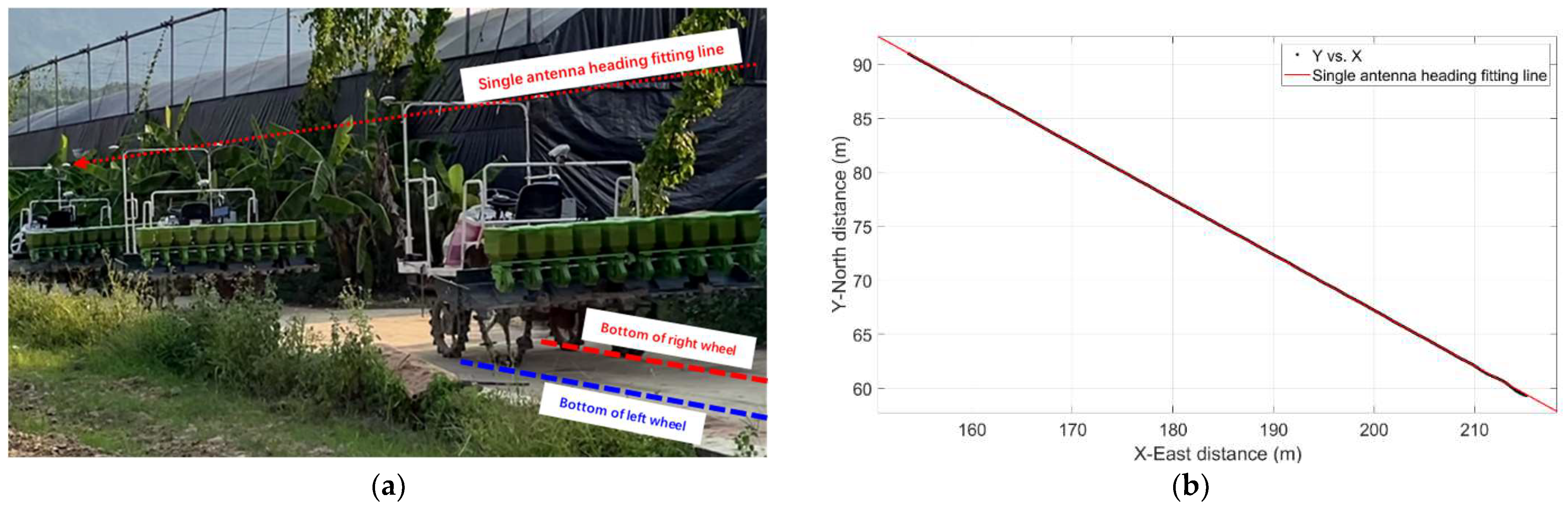
Automatic calibration of the heading angle
When the farm machinery travels in a straight line, the dual antennas record the heading value, and a point set for the main positioning antennas positioned in a straight travel trajectory is obtained at the same time. A straight line is fitted to the point set, and the direction of the fitted straight line is taken as the real heading of the farm machinery. The line model constructed using this fitting is shown in Equation (1):
y = k x + b
where x is the coordinate value of the main antenna positioned due east; y is the coordinate value of the main antenna positioned due north; k is the slope of the fitted line; and b is the intercept of the fitted line.
According to the single antenna heading linear fitting model, the true heading angle of the vehicle is the arctangent of the slope of the fitted straight line, as shown in Equation (2):
Y a w d = arctan ( k 180 π )
where Y a w d is the single-antenna heading angle.
The single-antenna heading angle is compared with the average value of the recorded dual-antenna heading angle, and the difference between the measured heading angle of the dual antenna and the real heading angle of the vehicle is obtained, that is, the installation error of the dual antenna is obtained, as shown in Equation (3):
E Y a w = Y a w d Y a w 0
where E Y a w is the installation error of the dual antenna and Y a w 0 is the average of the recorded heading angle of the dual antenna.
Therefore, the real-time true heading angle of the farm machinery is:
Y a w = Y a w 1 + E Y a w
where Y a w is the real-time true heading of the farm machine and Y a w 1 is the real-time collected heading of the farm machine.
(2)
Automatic calibration of the roll angle and pitch angle
We use the method for round-trip, straight-line driving of the agricultural machine following the same path, i.e., driving along the same path once in the positive direction and once in the negative direction. When driving in the positive direction, the value of the positive direction’s traverse angle and the value of the pitch angle are recorded, and when driving in the negative direction, the value of the negative direction’s traverse angle and the value of the pitch angle are recorded. Half of the average value of the round-trip traverse angle is the installation deviation angle of the sensor relative to the traverse angle of the vehicle body, as shown in Equation (5). Similarly, half of the average value of the round-trip pitch angle is also the installation deviation angle of the sensor relative to the vehicle body pitch angle, as shown in Equation (6).
E r o l l = ( i = 1 n roll- P i n + i = 1 n roll- N i n 2 ) = - ( roll- P 1 + roll- P 2 + roll- P n ) + ( roll- N 1 + roll- N 2 + roll- N n ) 2 n
where E r o l l is the roll angle measurement error; roll- P i is the i-th roll angle value for the positive direction of travel; n is the sample capacity; and roll- N i is the i-th roll angle value for the negative direction of travel.
E p i t c h = - ( i = 1 n pitch- P i n + i = 1 n pitch- N i n 2 ) = - ( pitch- P 1 + pitch- P 2 + pitch- P n ) + ( pitch- N 1 + pitch- N 2 + pitch- N n ) 2 n
where E p i t c h is the pitch angle measurement error; pitch- P i is the i-th pitch angle value for the positive direction of travel; n is the sample capacity; and pitch- N i is the i-th pitch angle value for the negative direction of travel.
Therefore, the real-time true roll angle of the agricultural machine is:
r o l l = r o l l 1 + E r o l l
where r o l l is the real-time roll angle of the farm machine and r o l l 1 is the real-time collected roll angle of the farm machine.
The real-time true pitch angle of the farm machine is:
p i t c h = p i t c h 1 + E p i t c h
where p i t c h is the real-time true pitch angle of the farm machine and p i t c h 1 is the real-time pitch angle of the farm machine.

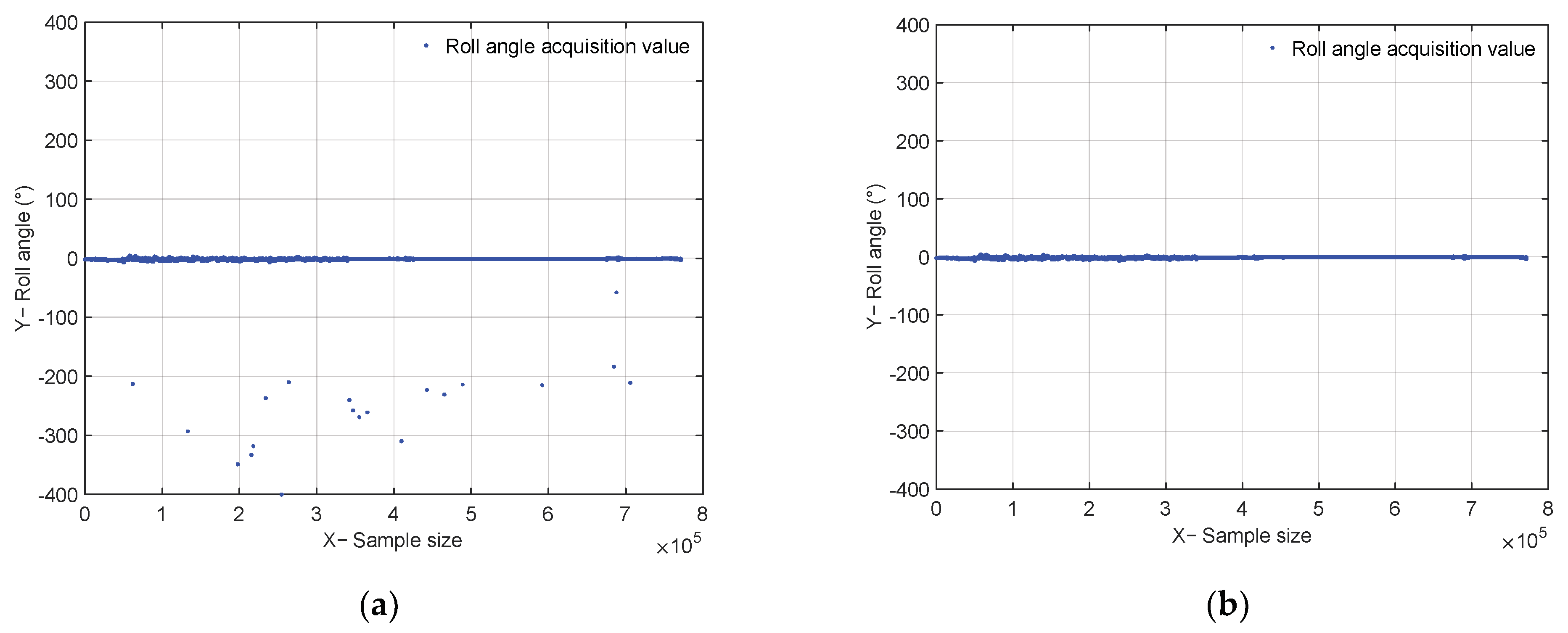
2.2.2. Outlier Rejection

Due to occasional data incompleteness or packet loss during data acquisition, in order to ensure the integrity of the collected hard layer contour information and intelligent agricultural machine operation data, the data acquisition module of the unmanned system was set to a 50 Hz acquisition frequency. Thus, each frame of data was repeated five times, and after de-emphasis, continuous and complete 10 Hz sensor information and operation real-time parameter data were obtained. The data frames are prone to anomalies and incomplete data preservation due to a large amount of data and because the system needs to start and stop in special circumstances during operation, resulting in ghost points during the acquisition process [29]. Such anomalies occur in the attitude sensor data acquisition process, where there are more coarse points of anomalous values in the acquisition of the transverse roll angle and pitch angle, and these are observed in the timing samples. These points show abnormally large deviations in the data in the direction of the longitudinal axis, causing the rear wheels’ bottom trajectory and the constructed hard bottom contour to show sharp protrusions in the constructed hard bottom contour, which cannot accurately express the true hard bottom contour characteristics. In order to avoid the influence of anomalies in the hard bottom contour feature extraction, this study used the Lajda criterion to remove outliers from the raw data on the attitude sensor transverse roll angle and pitch angle measurements. The principle is to first assume that a set of detection data contains only random errors and then calculate and process them to obtain the standard deviation σ and, finally, set the probability interval to which the confidence value belongs and consider the errors beyond this interval as suspicious data. Here, the probability interval is set as [−3σ, 3σ], and any data beyond this error were removed.
The roll angle and pitch angle measurements are both continuous with equal precision, and the anomalies were rejected separately by setting the measurement data set as { X 1 , X 2 , , X i } ( i = 1 , 2 , , n ) and M as their respective arithmetic averages. M is calculated as shown in Equation (9); the standard deviation σ is calculated according to Bessel’s formula, as shown in Equation (10). If a measurement value X i satisfies Equation (11), the point is considered a rough point and is rejected.
M = i = 1 n X i n = X 1 + X 2 + X n n
σ = 1 n i = 1 n ( X i M ) 2
| X i M | > 3 σ

2.2.3. Contour Trajectory 3D Spline Curve Denoising

Since the positioning error of the RTK-GNSS positioning system is 1.5 cm + 1 ppm in elevation, the raw data on the hard bottom contour trajectory collected with the rear wheels of the farm machinery are continuously “sawtooth” on the temporal chart. When the intelligent farm machinery encounters unexpected situations during operation that causes it to stop or move at a very low speed, according to the emergence of the suspended representative contour trajectory of the operation (Figure 2a), the 3D spline curve for the trajectory composed of the collected contour points is prone to self-crossing where two points overlap, as shown in Figure 2b. The actual contour should be a continuous spline curve contour, and there is no self-crossing in the front and back spatial point connection, so the real hard bottom local contour 3D spline trajectory is obtained using sliding denoising of the collected raw data without affecting the acquisition accuracy. Therefore, in this paper, the moving average and wavelet denoising [30] were used for the comparative analysis of local acquisition contour processing, and the results are shown in Figure 2.
According to the processing results in Figure 3, we can see that although the moving average filtering can remove the “sawtooth” noise in the hard bottom contour, the cost is that the original contour details are lost. For example, the original contour shows mutation and texture, but the mean filtering will lose these details, causing the hard bottom contour to become too smooth, as shown in Figure 3a. Wavelet denoising has the advantage of multi-resolution analysis. For the analysis of hard bottom contour features, such as non-smooth signals, in the case of contours with edges or abrupt elevation changes, the wavelet can be decomposed into different resolutions (scales) to deal with them separately, as shown in Figure 3b. That is, the “sawtooth” noise and self-phase intersection set of the hard bottom contour can be removed. Wavelet decomposition can also ensure the authenticity of the processed abrupt changes in the local hard bottom contour elevation or edge information to obtain a 3D spline curve of the local contour trajectory.

2.3. Hard Bottom Layer Surface Roughness Estimation Method

In order to quickly and continuously measure the hard substrate roughness with an intelligent farm machine traveling in real time, this section uses the hard substrate profile within the set length as the local roughness measurement range; that is, the hard substrate roughness measured with the farm machine at each moment is the roughness value measured from the previous moment to the set length of the traveling moment. The sampling method is shown in Figure 4. The uniform operating speed and data collection frequency set by the intelligent farm machine are known, so the total number of data frames from the previous moment to the present moment can be calculated. The calculation formula is shown in Equation (12):
n z = L / v f
where n z is the number of data frames from a previous moment to the present moment; L is the sampling length in m; v is the operating speed in m/s; and f is the acquisition frequency in Hz.
Using the hard bottom contour information collected with the intelligent farm machine chassis, a straight line is fitted with the least squares index method within a locally set length range, and the height of each point from this fitted line is calculated to provide input for calculating the surface roughness. The method can be applied to both flat and sloping land. Diagrams showing the relationship between the hard bottom contour, local fitted line segment, and contour point fitted to a straight-line height for flat and sloping land are shown in Figure 5a,b respectively.
Let the expression of the locally fitted straight line based on the least squares fit be:
y 1 = A x 1 + B
where y 1 is the height value of the upper point of the fitted line; x 1 is the contour point number value; A is the slope of the fitted line; and B is the intercept of the fitted line.
Let the distance from the i-th contour point in the local range to the fitted straight line be S i ; then, we have:
S i = | A n i z i + B | A 2 + B 2
where S i is the distance from the i-th contour point to the fitted line; n i the i-th contour point serial number; and z i is the i-th contour point height.
Then, let the local surface roughness at the j-th point of the hard bottom layer be R d j , which is calculated as follows:
R d j = 1 n z 0 n z | S | d x
Since the collected hard bottom layer is a discrete point, it can be approximated as:
R d j = 1 n z i = 1 n z | S i |
According to Equation (16), the local surface roughness characteristics of the hard bottom contour for the whole area of the farm machine can be obtained by traversing the hard bottom layer collected from the whole area of operation.

3. Results

3.1. Test Scenario

The paddy hard bottom layer contour sensing module was integrated into an unmanned agricultural machinery system, and the unmanned direct rice seeding machine was used to perform an unmanned mechanical seeding operation and collect the contour of the paddy hard bottom layer in the unmanned rice farm in Zengcheng District, Guangzhou City, South China Agricultural University. The planned operation path of the direct seeding machine is shown in Figure 6a, and the operation site is shown in Figure 6b.
The heading angle calibration was carried out in the straight-line driving section of the unmanned agricultural machine, and the method for the automatic calibration of the heading angle was used, as described in Section 2.2.1. The results of the line model constructed by fitting the trajectory of the main positioning antenna for straight-line driving are shown in Figure 7, Equation (17), and Table 1.
y = 0.5146 x + 170.1
According to the linear fitting model for the single-antenna heading angle, the slope k was −0.5146, and according to Equation (2), the true heading angle of the car body Y a w d was 152.77°, and the recorded heading average of the dual antenna Y a w 0 was 151.0711°. According to Equation (3), the fixed installation deviation of the dual antenna and the car body E Y a w was 1.6989°, so according to Equation (4), the true heading angle of the car body Y a w was the dual satellite antenna heading angle measurement value Y a w 1 plus 1.6989°.
Automatic calibration of the roll angle and pitch angle was carried out in the unmanned seeder’s round-trip, straight-line driving section. The farm machine was driven once along the same path in the positive direction and once in the negative direction, and the automatic calibration method for the roll angle and pitch angle described in Section 2.2.1 was used. The recorded rear wheel trajectory diagrams are shown in Figure 8a,b, respectively, and the average values for the collected roll angle and pitch angle and were calculated according to Equations (5) and (6). The obtained measurement error results are shown in Table 2.
According to Equations (7) and (8) and Table 2, the real-time true roll angle r o l l of the farm machine was the real-time collected roll angle r o l l 1 of the farm machine plus 0.04 degrees, and the real-time true pitch angle p i t c h of the farm machine was the real-time collected pitch angle p i t c h 1 plus 2.08 degrees.
In total, 772013 data acquisitions were performed. Outliers occurred in the roll angle acquisition 22 times, non-continuously and irregularly, and outliers occurred in the pitch angle acquisition 48 times, non-continuously and irregularly. Using the outlier rejection method described in Section 2.2.3, the results for the roll angle and pitch angle acquisitions before and after outlier rejection are shown in Figure 9, and the constructed rear wheel bottom trajectory and constructed hard bottom profile before and after outlier rejection are shown in Figure 10.

3.2. Quantitative Estimation of Hard Bottom Profile Roughness Characteristics for Whole Fields

The hard bottom surface roughness estimation method was used to estimate the whole field block. The estimated hard bottom contour surface roughness eigenvalues are associated with the positioning information, and the digital model for the whole field’s local roughness was constructed as shown in Figure 11. The digital model can provide a speed control reference basis for the intelligent farm machine: a larger feature value indicates a rougher local surface on the hard substrate layer, and it is recommended to reduce the operation speed accordingly in this position to ensure the quality of the operation. A smaller feature value indicates that the hard substrate layer is relatively flat, and it is recommended to increase the operation driving speed accordingly in this position to improve the operation efficiency, thereby improving the operation speed and quality of the intelligent farm machine as a whole.
The distribution of local roughness values was analyzed using the whole-field local roughness digital characteristic model, and the results are shown in Figure 12. The mean value for the whole-field local roughness of the test water field was 0.0065, where 68.27% of the local roughness values were distributed in the interval of [0.0042, 0.0087] and 99.73% were distributed in the interval of [0, 0.0133]. In addition, the higher frequency of measured local roughness in the interval of [0.0008, 0.002] was due to the longer idle stopping time and repeated acquisitions at the same location.

3.3. Representative Hard Bottom Contour Surface Characterization

According to the unmanned seeder’s heading angle change characteristics and the corresponding driving trajectory, a representative driving route from the hangar to the field, including transportation, down-field, operation, trapping, etc., was selected. The roughness characteristics of different hard bottom contours obtained after driving the agricultural machine were analyzed, where “①” marks the straight downhill driving section of the cement road; “②” marks the idle stop section; “③” marks the straight driving section on the flat cement road; “④” marks the section used to driving into the entrance of the field; “⑤” marks the normal straight-line driving operation section in the paddy field; and”⑥” marks the section for trapped vehicles. The route of the machine body’s heading changes is shown in Figure 13, and the trajectory is shown in Figure 14.
Using the hard bottom sliding surface roughness estimation method, we calculated the hard bottom local surface roughness for each driving section. All six cases of the driving hard bottom local surface roughness characteristics are shown in Figure 15, Figure 16, and Table 3. According to the measured roughness results for each driving segment, when the smart farm machine was in the idle state, where there was no elevation change in the wheel bottom measurement elevation, the measured surface roughness value was the lowest at 0.0011. This was followed by the road surface roughness value of 0.0023 collected on the flat and straight cement road, which was less than the value of 0.0037 collected on the straight downhill cement road. The surface roughness of the water field operation segment was greater than the cement road at 0.007. In the inlet section, because of the transition from dry paddy to wet paddy, the contour elevation difference was larger, so the surface roughness measured in this section was 0.0951, which was larger than the roughness of normal operation in paddy. In the trap section, because the local hard bottom contour elevation drops sharply, the measured roughness value was the largest at 0.1236.
When the intelligent agricultural machine drives on different road sections to collect hard bottom contours, the stepless classification of road conditions in different situations is realized according to the variability in the local surface roughness values, which can provide a reference basis for the motion control of an unmanned system vehicle.

4. Discussion

It is of great significance to study methods for quantifying the local characteristics of the hard bottom contour when driving intelligent agricultural machines and to analyze the local hard bottom conditions so as to provide real-time environmental feedback and realize the precise, high-quality, and efficient operation of unmanned agricultural machines.
It is difficult to quantify and express the local features of the hard bottom layer of paddy fields maneuvered by unmanned intelligent farming machines. This paper addresses this problem and proposes a method to quantify the local features of the hard bottom layer contour obtained when driving an intelligent farming machine using an unmanned direct seeding machine equipped with GNSS and AHRS as the hard bottom layer contour sensing platform. This method is applicable to wheeled agricultural machines without shock-absorbing suspension on the rear axle, such as rice transplanters and tractors, etc. This paper performed automatic calibration of the position and attitude sensors on intelligent farming machines, which reduces sensor installation precision requirements and calibration difficulties. In view of the problem that the unmanned system collects data prone to flypoints, this study rejected abnormal values in the collected hard bottom layer data, constructed a global roughness distribution model with associated position information based on the acquired hard bottom layer contour data, and obtained the surface roughness features at any position of the field. The results can provide environmental feedback parameters for the unmanned operation of intelligent farming machines, a reference for adaptive speed control of intelligent farming machines, and the quality and efficiency of their operation. The variability in contour features in the automatic transfer route of the unmanned intelligent farm machine from the hangar to the field was analyzed, and the results can provide a basis for the operation and control parameters to be used in unmanned operations to improve the operation efficiency in each segment.
The method designed in this paper, for the convenience of mechanical structure transformation design, used the position measurement sensor installed on the original mechanism of the water field agricultural machine as the contour sensing platform. There was a small amount of vibration in the positioning antenna in bumpy environments, and if the installation structure stiffness and installation accuracy can be improved, then we can further improve the measurement accuracy and reduce the number of sensor position correction steps. In this paper, the hard bottom layer contour of the paddy field was acquired using a fixed intelligent farm machine speed of 0.65 m/s, and the specific length of a 2 m range was used to extract the local contours. These parameters are suitable to distinguish the characteristics of different hard bottom layer contours, and if the speed of the intelligent farm machine can be correlated, then the corresponding length range contour can be adaptively selected for contour feature extraction under different speeds, which can further improve the adaptability of different farm machines. In addition, the method proposed in this paper was based on the digital modeling of hard bottom contours to calculate the local features of the whole area, which requires a large amount of calculation, and thus the background calculation is used. Further consideration needs to be given to the hard bottom characteristics of adjacent fields as they pass over the ridges [31], and this is also one of our future research directions.

5. Conclusions

The hard bottom layer of a paddy field where the unmanned operation of intelligent farming machines occurs is complex, and different features, such as potholes, have a great impact on the driving stability and the operation quality and efficiency of intelligent farming machines. It is difficult to ensure the stability of an unmanned operation path tracking the control of intelligent farm machines operating in fields with large differences in their hard bottom layer contour characteristics. The sensor installation position of the hard substratum sensing platform is random, and the collected data are prone to flypoints, which makes it difficult to realize the continuous quantitative expression of the local features of the hard substratum of paddy fields. This increases the difficulty in analyzing the contour features of the hard substratum of paddy fields. In addition, there is also a lack of quantitative expression methods for the local features of the hard substratum of paddy fields. In view of the above problems, this paper carried out experimental research and designed a method for the quantification of local features of the hard substratum contour obtained when driving intelligent farm machinery. This mainly includes:
(1)
The design of data processing methods for the automatic calibration of the sensor installation error, outlier rejection, and 3D spline curve denoising of contour trajectory. The real heading angle is obtained using the trajectory of the main positioning antenna of the intelligent farm machine in a straight line and fitting it to a straight line, and the difference is calculated and compensated for by comparing it with the installed dual-antenna directional acquisition heading angle to realize the heading calibration. The system error in the round-trip roll angle and pitch angle is obtained using the round-trip straight-line driving of the intelligent farm machine following the same path, and the calibration of the roll and pitch angle is realized. The raw data from the sensor measurements are processed using the Lajda criterion and the wavelet denoising method, and the rejection of the hard bottom contour ghost points and intersection points is realized with the intelligent farm machine’s data collection.
(2)
A quantification method for the local features of the hard bottom layer was established. Based on the field operation of unmanned live broadcasters and the simultaneous collection of hard bottom layer information, the local feature quantification of the hard bottom layer of paddy fields with correlated location information was achieved by calculating local sliding surface roughness to evaluate the degree of the hard bottom layer’s surface bumps. The quantified local characteristics of the hard bottom layer in the test plots showed that the mean value of local roughness was 0.0065, where 68.27% was distributed in the interval of [0.0042, 0.0087] and 99.73% was distributed in the interval of [0, 0.0133].
(3)
The variability in the surface roughness of the representative driving sections was analyzed. The hard bottom surface profile feature evaluation method based on local sliding surface roughness was used to analyze the hard bottom surface roughness features of the representative driving routes such as transport, down-field, operation, and trapping of the unmanned intelligent agricultural machine. It was used to compare the representative driving section profile’s feature variability based on the local surface roughness and proved the feasibility of the quantification method for the local features of the hard bottom layer.
The method for quantifying the hard bottom local features when driving an intelligent agricultural machine can provide feedback on the local environmental features of its unmanned operation at a current location. The results can provide a reference for the optimization of unmanned systems designed to improve the efficiency and quality of intelligent agricultural machine operations.

Author Contributions

Conceptualization, T.T., L.H., X.L. and J.H.; methodology, T.T., L.H., X.L. and J.H.; software, T.T., L.T., G.C., W.C., M.L. and Y.L. (Yuxuan Liu); validation, T.T., Z.M., D.F., K.H. and L.Z.; formal analysis, T.T.; investigation, T.T. and Y.L. (Yuqin Li); resources, T.T., L.H., X.L., J.H. and P.W.; data curation, T.T., L.H. and J.H.; writing—original draft preparation, T.T.; writing—review and editing, T.T., L.H., X.L. and J.H.; visualization, T.T., L.H., P.W. and M.Y.; supervision, L.H., X.L. and J.H.; project administration, X.L.; funding acquisition, X.L., L.H. and J.H. All authors have read and agreed to the published version of the manuscript.

Funding

This research was funded by the National Key Research and Development Program of China (Grant No.2021YFD2000602), the Jiangxi Provincial Science and Technology Special Project of Jinggangshan Agricultural High-tech Zone (Grant No.20222-051252), and the National Natural Science Foundation of China (Grant No.32071913; No.32101623).

Data Availability Statement

The data that support this study will be shared upon reasonable request to the corresponding author.

Acknowledgments

We would like to thank our partners at the Zengcheng Teaching Base of South China Agricultural University for their help and support in field management and machine maintenance.

Conflicts of Interest

The authors declare no conflict of interest.

References

  1. Nawaz, A.; Rehman, A.U.; Rehman, A.; Ahmad, S.; Siddique, K.H.M.; Farooq, M. Increasing sustainability for rice production systems. J. Cereal Sci. 2022, 103, 103400. [Google Scholar] [CrossRef]
  2. Kuenzer, C.; Knauer, K. Remote sensing of rice crop areas. Int. J. Remote Sens. 2013, 34, 2101–2139. [Google Scholar] [CrossRef]
  3. Xin, F.; Xiao, X.; Dong, J.; Zhang, G.; Zhang, Y.; Wu, X.; Li, X.; Zou, Z.; Ma, J.; Du, G.; et al. Large increases of paddy rice area, gross primary production, and grain production in Northeast China during 2000–2017. Sci. Total Environ. 2020, 711, 135183. [Google Scholar] [CrossRef]
  4. Zhao, Y. Statistical analysis of the changes of cultivated land resources in the past 10 years. Territ. Nat. Resour. Study 2020, 1, 53–57. [Google Scholar] [CrossRef]
  5. Liu, C.; Lin, H.; Li, Y.; Gong, L.; Miao, Z. Analysis on status and development trend of intelligent control technology for agricultural equipment. Nongye Jixie Xuebao/Trans. Chin. Soc. Agric. Mach. 2020, 51, 1–18. [Google Scholar] [CrossRef]
  6. Chen, X.; Wen, H.; Zhang, W.; Pan, F.; Zhao, Y. Advances and progress of agricultural machinery and sensing technology fusion. Smart Agric. 2020, 2, 1–16. [Google Scholar] [CrossRef]
  7. Luo, X.; Liao, J.; Zang, Y.; Ou, Y.; Wang, P. Developing from Mechanized to Smart Agricultural Production in China. Strateg. Study Chin. Acad. Eng. 2022, 24, 46–54. [Google Scholar] [CrossRef]
  8. Luo, X.; Liao, J.; Hu, L.; Zhou, Z.; Zhang, Z.; Zang, Y.; Wang, P.; He, J. Research progress of intelligent agricultural machinery and practice of unmanned farm in China. J. South China Agric. Univ. 2021, 42, 8–17. [Google Scholar] [CrossRef]
  9. He, J.; Hu, L.; Wang, P.; Liu, Y.; Man, Z.; Tu, T.; Yang, L.; Li, Y.; Yi, Y.; Li, W.; et al. Path tracking control method and performance test based on agricultural machinery pose correction. Comput. Electron. Agric. 2022, 200, 107185. [Google Scholar] [CrossRef]
  10. Hu, L.; Luo, X.; Lin, C.; Yang, W.; Xu, Y.; Li, Q. Development of 1PJ-4.0 laser leveler installed on a wheeled tractor for paddy field. Nongye Jixie Xuebao/Trans. Chin. Soc. Agric. Mach. 2014, 45, 146–151. [Google Scholar]
  11. Li, H.; Niu, D.; Wang, Y.; Li, X.; Meng, Q.; Liu, G. Rapid survey technology of farmland terrain based on RTK-GNSS. J. China Agric. Univ. 2014, 19, 188–194. [Google Scholar] [CrossRef]
  12. Hu, L.; Yang, W.; Xu, Y.; Zhou, H.; Luo, X.; Ke, X.; Zi, S. Design and experiment of paddy field leveler based on GPS. J. South China Agric. Univ. 2015, 36, 130–134. [Google Scholar] [CrossRef]
  13. Liu, G.; Li, X.; Kang, X.; Xia, Y.; Niu, D. Automatic Navigation Path Planning Method for Land Leveling Based on GNSS. Nongye Jixie Xuebao/Trans. Chin. Soc. Agric. Mach. 2016, 47, 21–28. [Google Scholar] [CrossRef]
  14. Xia, Y.; Liu, G.; Kang, X.; Jing, Y. Optimization and Analysis of Location Accuracy Based on GNSS-controlled Precise Land Leveling System. Nongye Jixie Xuebao/Trans. Chin. Soc. Agric. Mach. 2017, 48, 40–44. [Google Scholar] [CrossRef]
  15. Rovira-Más, F.; Zhang, Q.; Reid, J.F. Stereo vision three-dimensional terrain maps for precision agriculture. Comput. Electron. Agric. 2008, 60, 133–143. [Google Scholar] [CrossRef]
  16. Marinello, F.; Pezzuolo, A.; Gasparini, F.; Arvidsson, J.; Sartori, L. Application of the Kinect sensor for dynamic soil surface characterization. Precis. Agric. 2015, 16, 601–612. [Google Scholar] [CrossRef]
  17. Yandun Narváez, F.; Gregorio, E.; Escolà, A.; Rosell-Polo, J.R.; Torres-Torriti, M.; Auat Cheein, F. Terrain classification using ToF sensors for the enhancement of agricultural machinery traversability. J. Terramechanics 2018, 76, 1–13. [Google Scholar] [CrossRef] [Green Version]
  18. Zhang, M.; Chen, Y.; Jia, W.; Wang, M. Design of three dimensional topographic information measuring system. J. Jilin Univ. (Eng. Technol. Ed.) 2007, 37, 1451–1454. [Google Scholar] [CrossRef]
  19. Starek, M.J.; Chu, T.; Mitasova, H.; Harmon, R.S. Viewshed simulation and optimization for digital terrain modelling with terrestrial laser scanning. Int. J. Remote Sens. 2020, 41, 6409–6426. [Google Scholar] [CrossRef]
  20. Tu, T.; He, J.; Luo, X.; Hu, L.; Wang, P.; Chen, G.; Tian, L.; Feng, D.; Wang, Z.; Man, Z.; et al. Methods and experiments for collecting information and constructing models of bottom-layer contours in paddy fields. Comput. Electron. Agric. 2023, 207, 107719. [Google Scholar] [CrossRef]
  21. Flintsch, G.W.; Valeri, S.M.; Katicha, S.W.; de Leon Izeppi, E.D.; Medina-Flintsch, A. Probe vehicles used to measure road ride quality: Pilot demonstration. Transp. Res. Rec. 2012, 2304, 158–165. [Google Scholar] [CrossRef]
  22. Liu, Y.; Wang, G.; Yang, Y.; Liu, J.; Sun, L. Road surface equivalent reconstruction based on measured road spectrum. Trans. Chin. Soc. Agric. Eng. 2012, 28, 26–32. [Google Scholar] [CrossRef]
  23. Choi, M.; Kim, M.; Kim, G.; Kim, S.; Park, S.; Lee, S. 3D scanning technique for obtaining road surface and its applications. Int. J. Precis. Eng. Manuf. 2017, 18, 367–373. [Google Scholar] [CrossRef]
  24. Hou, Z.; Lu, Z.; Zhao, L. Fractal behavior of tillage soil surface roughness. Trans. Chin. Soc. Agric. Mach. 2007, 38, 50–53. [Google Scholar]
  25. Lu, Z.; Zhao, L.; Hou, Z. Fractal behavior of road profile roughness. J. Jiangsu Univ. (Nat. Sci. Ed.) 2008, 29, 111–114. [Google Scholar]
  26. Wang, L.; Yan, J.; Hou, Z.; Zhang, Y. Design and experiment on agricultural field profiling apparatus. J. Shenyang Agric. Univ. 2018, 49, 425–432. [Google Scholar] [CrossRef]
  27. Zhu, S.; Ma, J.; Yuan, J.; Xu, G.; Zhou, Y.; Deng, X. Vibration characteristics of tractor in condition of paddy operation. Trans. Chin. Soc. Agric. Eng. 2016, 32, 31–38. [Google Scholar] [CrossRef]
  28. Zhao, R.; Hu, L.; Luo, X.; Zhou, H.; Du, P.; Tang, L.; He, J.; Mao, T. A novel approach for describing and classifying the unevenness of the bottom layer of paddy fields. Comput. Electron. Agric. 2019, 162, 552–560. [Google Scholar] [CrossRef]
  29. Balduzzi, M.A.; Van der Zande, D.; Stuckens, J.; Verstraeten, W.W.; Coppin, P. The properties of terrestrial laser system intensity for measuring leaf geometries: A case study with conference pear trees (Pyrus Communis). Sensors 2011, 11, 1657–1681. [Google Scholar] [CrossRef]
  30. Sardy, S.; Tseng, P.; Bruce, A. Robust wavelet denoising. IEEE Transactions on Signal Processing. 2001, 49, 1146–1152. [Google Scholar] [CrossRef] [PubMed] [Green Version]
  31. Li, Y.; Wu, T.; Xiao, Y.; Gong, L.; Liu, C. Path planning in continuous adjacent farmlands and robust path-tracking control of a rice-seeding robot in paddy field. Comput. Electron. Agric. 2023, 210, 107900. [Google Scholar] [CrossRef]
Figure 1. Collection platform mounted on the chassis of an unmanned direct seeding machine.
Agronomy 13 01949 g001
Figure 2. Repeated and self-intersecting sets of points on job suspension: (a) representative contour trajectory and (b) continuous acquisition at the same position when the operation is suspended.
Agronomy 13 01949 g002
Figure 3. Comparison of moving average denoising and wavelet denoising: (a) moving average denoising and (b) wavelet denoising.
Agronomy 13 01949 g003
Figure 4. Sampling diagram.
Agronomy 13 01949 g004
Figure 5. Hard bottom contour, local fitted line segment, and contour point-to-fit straight line height relationship diagrams for (a) flat land and (b) sloping land.
Agronomy 13 01949 g005
Figure 6. Unmanned seeder planning operation path and site: (a) planned operational path and (b) operational site.
Agronomy 13 01949 g006
Figure 7. Unmanned seeder driving in a straight line and the main antenna position fitting a straight line: (a) test site, and (b) the straight line fit to the heading.
Agronomy 13 01949 g007
Figure 8. Round-trip linear trajectory under the same path: (a) forward travel trajectory and (b) reverse travel trajectory.
Agronomy 13 01949 g008
Figure 9. Attitude sensor acquisition value set: (a) the original set of values for roll angle acquisition; (b) the set of values for roll angle acquisition after removing outliers; (c) the original set of values for pitch angle acquisition; and (d) the set of values for pitch angle acquisition after rejecting outliers.
Agronomy 13 01949 g009aAgronomy 13 01949 g009b
Figure 10. Rear wheel bottom track and the hard bottom profile: (a) initial wheel track collected from the rear wheel bottom; (b) rear wheel bottom track after removing anomalies; (c) acquisition of the initial hard bottom contour; and (d) the hard bottom contour after removing outliers.
Agronomy 13 01949 g010
Figure 11. Digital feature model for the local roughness of the whole field.
Agronomy 13 01949 g011
Figure 12. Distribution of local roughness in the whole field.
Agronomy 13 01949 g012
Figure 13. Hangar-to-field transport and field operation heading angle of the unmanned seeder.
Agronomy 13 01949 g013
Figure 14. Hangar-to-field transport and field operation trajectory of the unmanned seeder.
Agronomy 13 01949 g014
Figure 15. Surface roughness characteristics for transport, down-field, operation, and trapping links: (a) ① concrete road on the downhill slope; (b) ② stopped and idling; (c) ③ flat concrete pavement; (d) ④ paddy field inlet; (e) ⑤ water field operation; and (f) ⑥ trap section.
Agronomy 13 01949 g015
Figure 16. Surface roughness of the representative driving section.
Agronomy 13 01949 g016
Table 1. Linear fit of the single-antenna heading angle.
Sample SizeR-SquareRMSESSEAdj R-sq
16,13510.00991.57611
Table 2. The mean and error of the cross-roll angle for round-trip straight driving and the driving cross-roll angle.
Roll Angle/°Pitch Angle/°
Average value (driving in the positive direction)0.197435−3.11529
Average value (driving in the negative direction)−0.27745−1.0474
Sensor mounting error0.040012.08134
Table 3. Surface roughness values for the representative driving section.
No.
Starting point number5056789310,00012,12614,78215,280
Termination point number6496932911,55712,26815,22916,001
Rd0.0037 0.0011 0.0023 0.0095 0.0070 0.0125
Disclaimer/Publisher’s Note: The statements, opinions and data contained in all publications are solely those of the individual author(s) and contributor(s) and not of MDPI and/or the editor(s). MDPI and/or the editor(s) disclaim responsibility for any injury to people or property resulting from any ideas, methods, instructions or products referred to in the content.

