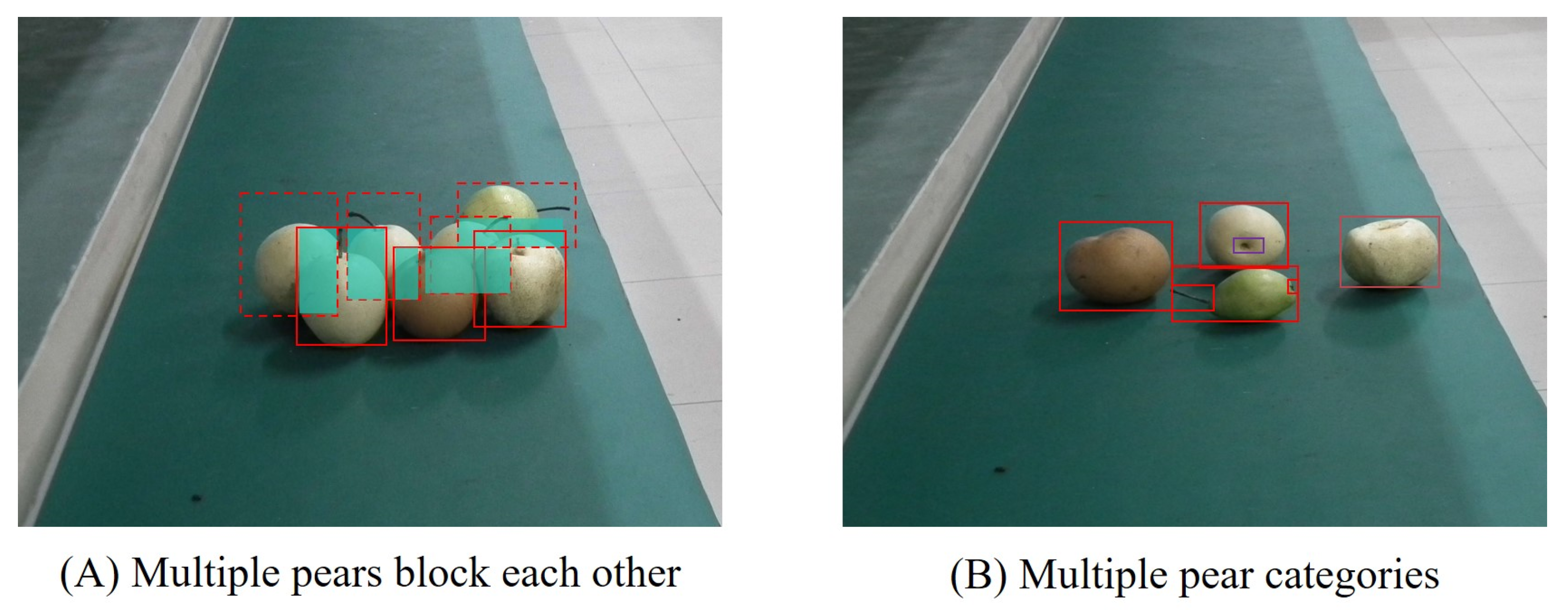
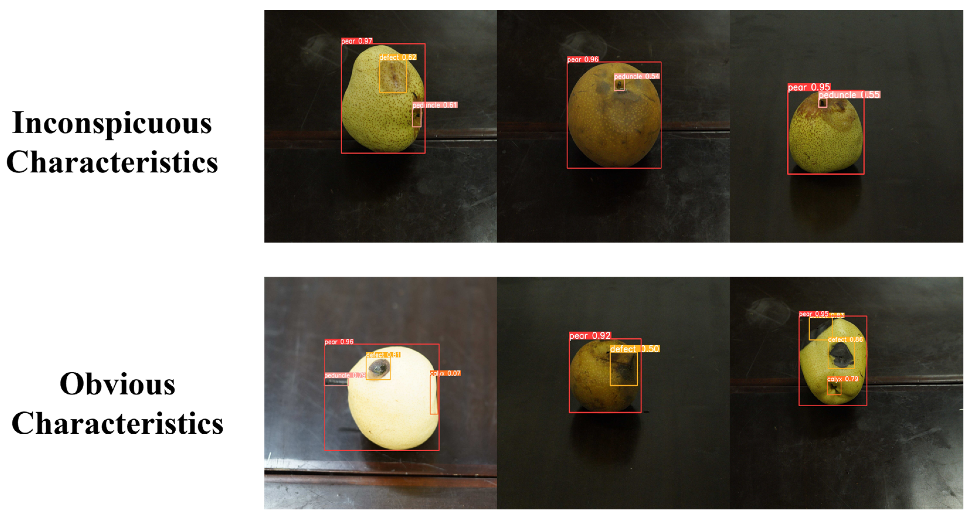
Article

ECLPOD: An Extremely Compressed Lightweight Model for Pear Object Detection in Smart Agriculture

1
College of Computer & Information Engineering, Central South University of Forestry and Technology, Changsha 410004, China
2
College of Food Science and Engineering, Central South University of Forestry and Technology, Changsha 410004, China
3
Department of Soil and Water Systems, University of Idaho, Moscow, ID 83844, USA
*
Authors to whom correspondence should be addressed.
Agronomy 2023, 13(7), 1891; https://doi.org/10.3390/agronomy13071891
Submission received: 7 May 2023 / Revised: 4 July 2023 / Accepted: 15 July 2023 / Published: 17 July 2023

Abstract

:
Accurate pear sorting plays a crucial role in ensuring the quality of pears and increasing the sales of them. In the domain of intelligent pear sorting, precise target detection of pears is imperative. However, practical implementation faces challenges in achieving adequate accuracy in pear target detection due to the limitations of computational resources in embedded devices and the occurrence of occlusion among pears. To solve this problem, we built an image acquisition system based on pear sorting equipment and created a pear dataset containing 34,598 pear images under laboratory conditions. The dataset was meticulously annotated using the LabelImg software, resulting in a total of 154,688 precise annotations for pears, pear stems, pear calyxes, and pear defects. Furthermore, we propose an Extremely Compressed Lightweight Model for Pear Object Detection (ECLPOD) based on YOLOv7’s pipeline to assist in the pear sorting task. Firstly, the Hierarchical Interactive Shrinking Network (HISNet) was proposed, which contributed to efficient feature extraction with a limited amount of computation and parameters. The Bulk Feature Pyramid (BFP) module was then proposed to enhance pear contour information extraction during feature fusion. Finally, the Accuracy Compensation Strategy (ACS) was proposed to improve the detection capability of the model, especially for identification of the calyces and stalks of pears. The experimental results indicate that the ECLPOD achieves 90.1% precision (P) and 85.52% mAP50 with only 0.58 million parameters and 1.3 GFLOPs of computation in the homemade pear dataset in this paper. Compared with YOLOv7, the number of parameters and the amount of computation for the ECLPOD are compressed to 1.5% and 1.3%, respectively. Compared with other mainstream methods, the ECLPOD achieves an optimal trade-off between accuracy and complexity. This suggests that the ECLPOD is superior to these existing approaches in the field of object detection for assisting pear sorting tasks with good potential for embedded device deployment.

1. Introduction

Pears are widely cultivated in Asia, Western Europe, North America, and other regions, with an annual output of nearly 25 million tons [1], making pears one of the five largest fruit in the world. Brilliant sales of pears mainly depend on the quality (appearance, taste, sweetness, acidity, and moisture) and postharvest commercialization of pears [2]. The quality of pear varies little, but the postharvest commercialization [3] of pears varies greatly. From the picking of pears to the postharvest commercialization of pears, the quality of pears will be affected by the packaging and transportation process. For example, bruised and rotten pears will decay untouched pears [4] in the packaging and transportation process. When pear quality does not meet consumer expectations, the demand in the market and sales may decline. This will cause the price of pears to fall, and farmers and other players in the industrial chain will face the risk of reduced income [5].
In order to ensure the quality of pears and increase sales, it is essential to carry out pear sorting.
As agriculture embraces modernization and intelligent technologies, deep learning has emerged as a crucial tool in the realm of fruit sorting. Through the application of deep learning techniques, researchers have developed neural network models that possess the ability to autonomously learn and discern the unique characteristics of fruits. During the sorting process, these models rapidly analyze fruit images, accurately identifying the position and specific attributes of each fruit. Leveraging this information, automated systems, such as robotic arms, can execute precise sorting strategies, thereby facilitating a highly efficient and effective fruit sorting process.
We tried to use YOLOv7 for an auxiliary pear sorting task. The network performs well in simple scenarios. However, in the actual automation-assisted pear sorting process, there are still the following three problems to be solved. (1) Deep learning models require a lot of computing resources and are difficult to deploy on low-cost embedded devices. (2) The pear groups are easy to occlude, as shown in Figure 1A, which leads to a large deviation between pear position during data collection and the pear position predicted by the model, resulting in missed detection. (3) Different types of pears have huge differences in shape, color, and body shape due to their different growth characteristics, as shown in Figure 1B, which makes it difficult for the model to learn the characteristics of pears and easily leads to false detection.
Aiming at the problem of deep learning models being difficult to deploy on low-cost embedded devices, Zhang et al. [6] chose the lightweight Light-CSPNet as the backbone network in the fruit detection task to adapt to the trade-off between model complexity and deployment. However, Jinpeng et al. [7] chose the Mobilenet-v3 network to replace CSPDarknet-53 in YOLOv4, which reduced the complexity of the backbone network. Although these improvements have achieved better results, the parameters in the network backbone are still too large. In order to reduce the amount of model parameters and save computing costs, we propose the Hierarchical Interactive Shrinking Network to solve the problem of excessive model complexity and difficult deployment. This module uses a hierarchical interactive shrinking mechanism to shrink and interact with features layer by layer. While maintaining low model complexity, key pear features are extracted.
Aiming at the problem of false detection caused by the mutual occlusion of fruits, Zheng et al. [8] proposed multi-task learning to solve the problem of mango picking. Through the joint action of MASK-RCNN and Faster-RCNN, it can effectively detect occluded mangoes. However, the joint action of the two models will bring a huge amount of calculation. For this reason, in solving the occlusion problem of camellia oleifera, Chen et al. [9] introduced a CA with a small amount of parameters by encoding the location information into the attention map, allowing the network to access information for a larger area and improving the network’s attention to the occlusion area. Considering the particularity of pear group features, we propose the Bulk Feature Pyramid (BFP) module to solve the occlusion problem in pear groups. The model uses the sparse reward and punishment mechanism to select the important features of the pear to reduce the interference of the detection of the pear occlusion pair.
Aiming at the problem of false detection caused by differences in fruit color and shape, Jia et al. [10] introduced a region of interest network (RPN) to optimize the feature extraction stage in fruit picking research to improve the model’s ability to adapt to differences in fruit color and shape. In addition, Wang et al. [11] chose YOLOv5s as the benchmark network in the real-time recognition of apple stems/calyces and used the pre-trained weights of the COCO dataset to enrich the feature representation of the model. Although these methods have improved detection accuracy to a certain extent, they have not made targeted improvements to the characteristics of the detection task. According to the characteristics of pears, this paper proposes a precision compensation strategy. Through iterative transfer learning, we let the model enrich the feature representation of large, medium, and small targets to adapt to the feature changes of pears, thereby reducing the risk of false detection.
The research contributions of this paper are as follows:
  • For the first time, we have created a large dataset specifically designed for pear sorting. The dataset comprises 34,598 pear images, encompassing both simple and complex scenarios, along with meticulously standardized and accurate pear labels totaling 154,688. This dataset aims to address the challenges in pear sorting and provide valuable data support for researchers in related fields conducting experiments.
  • In order to solve the problem of auxiliary pear sorting, we proposed the ECLPOD based on YOLOv7’s pipeline. The working flow of the network is shown in Figure 2.
    • We propose the HSINet module to compensate for the complexity of deep learning models that are difficult to deploy. The module functions in the feature extraction stage and extracts pear feature information efficiently with a small amount of computing resources.
    • We propose a BFP module to solve the problem of missed detections caused by pear group occlusion. The module uses sparsity reward and punishment to focus the model’s learning on the characteristic information of pears to alleviate the interference of redundant information and occlusion information in pear images.
    • We propose the ACS to compensate for the false detection problem caused by differences in the color and shape of pears. Iterative transfer learning was used to enrich the feature information of different scales for pear sorting.
  • In pear detection data, our ECLPOD only uses 0.5 M and 1.3 GFLOPs to reach the mAP50 of 85.2. Compared with other popular detection methods, our model achieves a trade-off between accuracy and model complexity and has more potential for practical deployment.
To facilitate reader comprehension, we have compiled a list of abbreviations and formula symbols used in this paper, as shown in Table 1 and Table 2, respectively.

2. Related Works

Pear sorting plays a crucial role in enhancing the overall quality of pears, boosting consumer demand, and improving the competitiveness and sustainability of the pear industry. Currently, there are primarily three methods used for pear sorting: (1) manual sorting methods or machine sorting methods, (2) integration of machine learning with sorting equipment, and (3) utilization of deep learning techniques in conjunction with sorting equipment.
In order to compensate for the shortcomings of mechanical sorting methods, the industry introduced computer vision to assist machine sorting in the fruit sorting process. Zhang et al. [12] proposed a mechanical sorting method based on fruit morphology, in which a mechanical arm grasps the stems of fruit bunches during the sorting process to protect fruit from damage. To improve the speed of fruit sorting, Dewi et al. [13] designed a fruit sorting robot that sorts based on color and size, which classifies fruit categories by fruit color thresholds and passes the above information to a robotic arm for fruit sorting. However, with too little fruit information, the RGB image makes it easy to miss the recognition of defects. Unay et al. [14] used multispectral images and computer vision to recognize defects in fruit. Even though these traditional computer vision methods have good recognition rates, they depend a lot on extracted features and classifiers. Some of them even require complex and expensive image acquisition equipment, which is hard to obtain with industrial inspection. Additionally, the detection speed of traditional visual methods is too slow to implement.
Recently, advancements in deep learning have introduced innovative approaches for addressing complex issues, with researchers applying these methods across a variety of domains, such as agriculture [15,16], industry [17], medicine [18,19], forest safety [20], and so on. Therefore, the application of deep learning technology to the field of fruit sorting has also received more and more attention. A summary of the sorting methods based on deep learning in recent years is shown in Table 3.
The above research shows that deep learning technology has excellent performance in fruit sorting tasks. However, previous studies focused on simple identification and classification of individual fruits and did not take into account the auxiliary role of fruit sorting in large-scale scenarios. In addition, for deep learning, data are crucial. Too small a dataset can lead to the risk of overfitting the model. Therefore, in order to cope with the complex pear sorting task in large-scale scenarios, we created a pear sorting dataset and selected the excellent YOLOv7 target detector as the benchmark network to realize the auxiliary pear sorting task in large-scale scenarios.

3. Materials and Methods

3.1. The Sample Used in the Experiment

In this paper, 468 common pear samples were purchased from the Red Star Fruit Wholesale Market in Changsha, China, as experimental samples, among which were 9 total varieties of pear: Sour pear (80), Crystal tribute pear (49), Pyrus pyrifolia (47), Korla fragrant pears (52), Gong pear (36), Crown pear (50), Dangshan pear (60), Fuchuan pear (39), and Pyrus nivalis (55). All samples were stored at room temperature (24–26 °C) for 24 h before the experiment. Pears were stored at room temperature after each image acquisition.

3.2. Data Acquisition Systems and Data Types

3.2.1. Data Acquisition Systems

In the field of pear sorting through auxiliary detection based on deep learning, there is no public pear sorting dataset at present. Therefore, our researchers built a sorting scenario to simulate the pear sorting process and made a large pear sorting dataset. The data collection equipment was composed of five cameras, including a Canon EOS 40D, SONYA6000L, SONY a7r3, PENTAXK-70, and Fujifilm HS11. By adjusting the tripod, the camera position was fixed at a height of 30 cm. The focal length of the camera was then fixed, and the pears were placed at a short distance (0.4 m), a medium distance (1.0 m), and a long distance (2.0 m). Various complex situations in the sorting process were simulated by changing pear attitude, pear type, pear quantity, and pear position, as shown in Figure 3E.

3.2.2. Data Acquisition

The dataset collected in this paper was mainly collected on the simulated sorting line. Considering the different data acquisition equipment on the sorting line, there may be differences in the collected images (size and clarity). Therefore, we used multiple cameras of different models to collect data and take pictures of various sizes and clarity. At the same time, we changed the combination of pear attitude and quantity to simulate complex situations in the practical application of sorting lines. Illumination conditions are crucial during data collection, as different light intensities can impact the color and texture features of pears in the images. For instance, excessive lighting can result in image distortion, while insufficient lighting can obscure the distinctiveness of pear features, as shown in Figure 3D. To mitigate this interference, we simulated scenarios with weak, strong, and normal lighting conditions.
This dataset is divided into four parts: a single pear location dataset, a pear location dataset with a limited number of pears, a multiple pear location dataset, and a complex pear location dataset. The specific types of datasets are shown in Figure 3. The pear images in this dataset include a variety of sizes, with resolutions of 2736 × 3648, 2656 × 3984, 2000 × 3008, 2048 × 3072, and 2592 × 3888. A total of 34,598 images were obtained, of which 29,195 were used to train and verify the model. Images were randomly divided according to a ratio of 7:3, and the remaining 5403 pieces were used for robustness analysis of the model.
For each image, the whole of each pear, the stem of the pear, the calyx of the pear, and the defects of the pear were marked using labelImg2-master [28]. See Table 4 for the number of label objects in the dataset.

3.3. YOLOv7

YOLO is one of the best algorithms in the field of object detection. YOLOv7 [29] adds an E-ELAN structure compared with the previous YOLO series, which improves the network’s ability to learn and makes it easier to identify pear features without destroying the original gradient path. In the head layer, the RepVGG style is introduced to transform the structure of the head network. In the training process, multiple branches can be used to improve the learning performance of pear features. In the detection process, the structure can be re-parameterized to accelerate the detection of pear features. In addition, YOLOv7 uses auxiliary head training for deep supervision of the model.
The YOLOv7 algorithm ensures the accuracy of pear sorting recognition. However, in industrial applications, the computing resources required by the model should be as small as possible. The number of model parameters for YOLOv7 is as high as 37.2 M, which is difficult to achieve in the model deployment process. Therefore, it is necessary to find a network model suitable for pear detection that strikes a balance between detection performance and model complexity.

3.4. ECLPOD for Assisted Pear Sorting

In the detection task of auxiliary pear sorting, the complexity of the model is too large, which makes it difficult to implement in practical applications. In addition, in the process of pear detection, the placement of the pear is random and it is easy to block other pears in the group during data collection, resulting in missed pear detections. At the same time, the features of different pears are obviously different, which easily causes interference in research into pear features and results in the false detection of pears, thus reducing identification accuracy.
To solve the above problems, a pear recognition and detection method, ECLPOD, is proposed based on YOLOv7’s pipeline. The network structure is shown in Figure 4. The network first proposes the use of the HIS module to reduce the computational complexity of the feature extraction process, and then proposes the use of the BFP module using the proposed LNBA to capture key pear edge features so as to reduce occlusion interference. Finally, the ACS was used to improve the model’s recognition accuracy.

3.4.1. Hierarchical Interactive Shrinking Network

It is required to identify pears quickly and accurately in the process of pear industrial sorting. However, when restricted to the memory and computing resources of embedded devices and edge devices, it is necessary to use limited computer resources to accomplish efficient feature extraction. The task of object detection relies heavily on feature extraction. It turns the input image into the deep-seated and high-semantic feature image based on the backbone of the convolution module. In YOLOv7, feature extraction uses an E-ELAN and MP structure with a high number of convolution modules and a large number of parameters and calculations, which is not suitable for industrial applications. Despite the superior performance achieved by YOLOv7 in assisting pear target detection, its feature extraction relies on E-ELAN and MP structures, incorporating numerous convolution modules. This results in a significant number of parameters and computations, which may hinder its practical deployment in industry.
In order to make the deep learning model more applicable for industrial deployment, we proposed the Hierarchical Interactive Shrinking Network (HISNet) based on the backbone of YOLOv7-tiny (as shown in Figure 4). The structure consists of three parts: the CBH, DW-Block, and GAD. Among them, the CBH uses 2D convolution to extract the feature and structure information of pear images and provides rich feature representation for subsequent layers; the DW-Block uses depth-separable convolution instead of original convolution to reduce the amount of parameters in the feature extraction process; and the GAD passes the GAP [30] and the dropout to compress feature information and reduce the connection of useless hidden layers in the network while using as limited a number of parameters as possible to identify pear features.
The specific improvements of HISNet are as follows:
  • To achieve a lower number of parameters and computational complexity during the feature extraction stage, we introduce the use of depthwise separable convolution in the DW-Block [31]. This approach enables large and complex neural networks to operate effectively with significantly reduced complexity. Depthwise separable convolution divides the convolution process into two steps, resulting in a much smaller parameter and computational footprint.
The first step involves performing a depthwise convolution on each channel of the input feature. This step applies a 2D convolution operation individually to each channel. It aims to extract features from each channel while preserving the same number of channels. The process can be represented by Equation (1).
y ( p 0 , c ) = p n R w ( p n , c ) × x ( p 0 + p n , c )
The next step involves pointwise convolution applied to the information processed by the depthwise convolution. It employs a 1 × 1 convolutional kernel to merge the features from each channel through a standard 3D convolution process. This step performs spatial convolution operations on the features at each position to capture more comprehensive spatial information. The process can be represented by Equation (2).
y ( p 0 ) = c = 1 C w ( c ) × y ( p 0 , c )
where x ( p 0 + p n ) is the value of the input feature at ( p 0 + p n ) , y ( p 0 , c ) represents the value at P 0 of the c channel feature map after deep convolution, y ( p 0 ) represents the value at position P 0 in the final output feature map, R is the effective receptive field area of the convolution kernel, w ( p n , c ) is the weight of depth convolution, and w ( c ) is the weight of point-by-point convolution.
Through the combination of deep convolution and pointwise convolution, depthwise separable convolution achieves efficient feature extraction with reduced computational and parameter requirements. To compare the computational costs of regular convolution and depthwise separable convolution, let us assume that the input feature map has a size of S i n × S i n and S c × S c channels, with a total of N convolution kernels. The computational costs for origin convolution (OC) and depthwise separable convolution (DSC) are given by Equations (3) and (4), as shown below.
O C = S i n × S i n × C × N × S c × S c
D S C = S i n × S i n × C × S c × S c + S i n × S i n × C × N
After calculation, the calculation ratio of depth separable convolution and ordinary convolution is
r a t i o = O C D S C = S i n × S i n × C × S c × S c + S i n × S i n × C × N S i n × S i n × C × N × S c × S c
It is evident that the reduction in computation for depthwise separable convolution is determined by the size of the two-dimensional convolution kernel and the number of three-dimensional convolution kernels employed. In practical applications, depthwise separable convolution commonly employs a 3 × 3 convolution kernel. For instance, if the number of output channels is set to 64, the computation required for depthwise separable convolution is only one-tenth of that for regular convolution.
2.
In the fully connected layer of the network, we propose the GAD module to replace the fully connected layer, as shown in Figure 4C. The fully connected layer is replaced by the GAP and the dropout. In the initial stage of the convolutional neural network, the convolution layer needs one or more fully connected layers after passing through the maximum pool layer, and Softmax classification is then adopted. However, the fully connected layer transforms the convolution layer into vectors, subsequently classifying each feature map. The parameters of the fully connected layer are too large, which leads to slow training speeds with datasets and models that overfit easily. Here, the GAP can pool the whole feature map evenly, compress the feature map into feature points, and classify the feature points. The GAP gives practical class meaning to each channel, regularizes the network structurally, introduces the dropout in network training, and randomly drops some neurons with a certain probability, which not only reduces parameters but also avoids overfitting caused by full connection.
In Section 4.5.1, we assess the feature extraction capabilities of the HISNet.

3.4.2. Bulk Feature Pyramid

In the process of pear sorting, the identification of multiple pears simultaneously is often employed to enhance market competitiveness and improve sorting efficiency. However, as the number of pears increases, mutual occlusion between pear groups becomes a common issue. This occlusion poses challenges in localization as the features of the occluded pears are easily overlooked by the detector.
To alleviate the pear feature occlusion problem, we propose a BFP module, as shown in Figure 4D. This module consists of three parts: the DW-block, C3-Block, and LNBA in the HSINet. The following is a description of the functions of these three parts.
DW-Block and C3-Block: These two components are primarily employed to minimize computational load and parameters in the process of model feature fusion, thereby achieving models that are lightweight. The DW-Block applies depthwise separable convolution, wherein the convolution operation is decomposed into depthwise and pointwise convolutions, effectively reducing calculation load. The C3-Block utilizes the CSP bottleneck structure, enhancing the network’s expressive capabilities through feature transformation and channel concatenation.
LNBA: This section utilizes a sparse reward and punishment mechanism to determine the significance of pear features, aiding the network in accurately identifying pear features and effectively locating obstructed pears. The human visual attention mechanism has the ability to concentrate on specific areas with a high level of detail while simultaneously processing irrelevant information in the surroundings with reduced clarity. Drawing inspiration from the human visual attention mechanism, LNBA replicates human visual characteristics and assigns importance to significant pear features, empowering the network to concentrate on the key aspects of pear features.
As shown in Figure 4D, LNBA first takes the feature map as the initial input and performs BatchNorm normalization on the feature map according to the complexity of the feature information. We assume that F i n and F o u t are input and output feature graphs, respectively, such as in Formula (6).
B N o u t = λ F i n μ F i n σ F i n 2 + ε + β
The feature maps are then adjusted according to the scaling factor in BatchNorm. This rewards important information in pear feature fusion and suppresses irrelevant information.
W e i g h t = γ i j = 0 γ j × B N o u t
Finally, to constrain the range of feature information, we introduce a learnable sigmoid function.
F o u t = α × s i g m o i d ( W e i g h t + φ )
where α and φ are the learning parameters of the affine transformation parameters of the sigmoid activation function and λ and β are learning parameters in the BN structure.
Compared to the traditional sigmoid function, the learnable sigmoid function extends the range of feature constraints from the original [0, 1] to the range of pear feature distribution. This constraint idea is inspired by ReacNet [32], which enables the sigmoid activation function to adjust based on data features and adapt to different feature representations. This constraint mechanism effectively expresses pear feature information, allowing the network to better focus on key features and address occlusion between pear clusters.
By integrating DW-Block, C3-Block, and LNBA, the BFP module is able to effectively alleviate the occlusion problem in pear detection. It reduces the computational and parameter complexity of the model, enhances the lightweight nature of the model, and leverages LNBA to focus on the main pear characteristic regions, thus improving occluded pear detection and localization performance. In order to measure the effectiveness of the BFP module, we verify the effectiveness of the combination of DW-Block and C3-Block in Section 4.5.2, and also verify the effectiveness of LNBA.

3.4.3. Accuracy Compensation Strategy

Pears belong to the dicotyledonous family Rosaceae. The fruit is either round or irregularly pear-shaped (thinner at the base and thicker at the tail). Different varieties of pear also show great changes in peel color, including yellow, green, yellow with green, green with yellow, and other colors, with some individual varieties even having purple peel. These differences in shape and color create challenges and distractions for pear target detection tasks.
In this paper, based on the features of pears themselves, the information bottleneck theory is applied to the neural network to make up for the deficiency in the lightweight network’s feature representation and narrow the information gap between the lightweight network and YOLOv7 so as to eliminate redundant information and efficiently mine the feature information of pears. The principle of the information bottleneck [33] is directly related to model compression, and its best assumption is to minimize information gain and model complexity, as shown in Equation (9).
min :   R I B ( α ) = I ( Z , Y ; α ) β I ( Z , X ; α )
where R I B ( α ) is the information bottleneck, α is the parameter of the network, I ( A , B ; α ) is the mutual information of input image B and feature information A, and I ( A , C ; α ) is the mutual information of input image C and feature information A.
The mutual information minimization method based on information bottleneck theory excludes redundant information unrelated to tasks from the compressed model so as to make full use of the capacity of lightweight models. According to the information bottleneck criterion, we designed two specific precision compensating strategies (iterative transfer learning and the Test Time Augmentation) to maximize the mutual information between the feature mapping of object detection and learning.
Iterative transfer learning
Due to the large differences in the shapes and colors of different pears, as well as the small calyces and defects in pears, if the model is directly used for training, the convolutional neural network with randomly initialized weights is not sufficient for the feature extraction of pears, which easily falls into the local optimal solution and struggles to achieve better results.
Transfer learning [34] was introduced to transfer the learned knowledge from the existing domain to the new domain so that the model could better perform the new task. For example, Wang et al. [11] transferred knowledge from the COCO [35] detection task to the apple detection task, which significantly improved the performance of apple detection. However, in the COCO dataset, there are too few features for small targets, and the model is not strong enough to learn the features of small targets. Therefore, we propose a new transfer learning method called iterative transfer learning (as shown in Figure 4E).
In the process of iterative transfer learning, we use the AITOD dataset to supplement small target features so that the model is iteratively trained under the COCO and AITOD datasets, thus fully learning the features of various targets. The specific process is as follows:
First, the model was pre-trained in the COCO task to enrich the model’s feature cognition of objects in natural scenes and improve the model’s feature recognition for medium and large targets.
M C O C O = P r e t r a i n ( C O C O )
The model was then further fine-tuned using the AITOD dataset to accommodate small target features.
M A I T O D F t = F i n e t u n e ( M C O C O , A I T O D )
Subsequently, the model makes a final tweak in the C O C O dataset, allowing the model to review the characteristics of the large and medium targets.
M C O C O F t = F i n e t u n e ( M A I T O D , C O C O )
Finally, COCO’s fine-tuned weights are put into the pear target task for training.
M P e a r D a t a = T r a i n ( M C O C O F t , P e a r D a t a )
where M represents the weight information after training. C O C O , A I T O D , and P e a r D a t a are respective proxies for datasets.
Test Time Augmentation
In order to compensate for the accuracy loss caused by making the model lightweight, the TTA (Test Time Augmentation) strategy [36] is adopted during the detection process. As shown in Figure 4E, test augmentation is performed on the input data, generating new images through scale transformation and flipping, with these generated images then inferred upon. After the inference is completed, the detection results of multiple images are averaged, effectively compensating for the insufficient recognition of important features in the original images during the detection process. The pseudo code flowchat example of TTA is shown below (Algorithm 1).
Algorithm 1. TTA
1Input: The input is original image I during detection
2Begin:
3      A f l i p I // flip original image
4      B s c a l e I // Scale the original image
5      D = a v e r a g e ( d e t e c t A , d e t e c t ( B ) ) //Detect transformed images and average them
6Return  D
7Output: The test result after TTA is D
The model’s performance in the pear target detection task can be improved by compensating for the strategy of accuracy, enabling the model to better understand and utilize the feature information of pears. The corresponding experiment is described in Section 4.5.3.

4. Results

This section evaluates and analyzes the effect of the algorithm from multiple dimensions, such as the ECLPOD’s performance, module effectiveness, ablation experiments, comparison with algorithms that perform well in the field of object detection, robust application tests, and practical application tests, and verifies that the ECLPOD can be used with effectiveness and superiority in the task of pear object detection.

4.1. Evaluation Indicators

To evaluate the performance of the model in the pear object detection task, we use precision (P), recall (R), F1score, mAP, FPS, parameter size, and GFLOPs.
The results are divided into two categories: P r e c i s i o n is the proportion of images correctly detected as positive samples compared to the total amount the model detected, and R e c a l l is the proportion of images correctly detected as positive samples compared to total number of true positive samples. The correlation formula is as follows:
P r e c i s i o n = T P T P + F P × 100 %
R e c a l l = T P T P + F N × 100 %
where T P is the true positive sample, F P is the false positive sample, and F N is the false negative sample.
F 1 s c o r e is used to evaluate the model’s performance, and the formula for F 1 s c o r e is as follows:
F 1 s c o r e = 2 × P r e c i s i o n × R e c a l l P r e c i s i o n + R e c a l l × 100 %
m A P is the standard for evaluating the object detection algorithm, which indicates the overall accuracy of the model. The formula is as follows:
m A P = 1 n u m j = 1 n u m A P j
A P = 0 1 ( P r e c i s i o n × R e c a l l ) d ( R e c a l l )
where j represents the part category of the pear and n u m represents the total number of categories. A P represents the average accuracy of a single category.
FPS serves as a metric for the detection speed of a model, signifying the average count of images analyzed per second. The formula is as follows:
F P S = 1 t
The inference time of a single picture is t.
Parameters are used to measure the size of the model, and as the number of parameters increases, the demand for computer memory also escalates. In the following equations, K denotes the size of the convolution kernel, C i n and C o u t represent the number of input and output channels, and I and O indicate the number of weights for input and output, respectively.
P a r a m C o n v = ( K × C i n + 1 ) × C o u t
P a r a m F C = ( I + 1 ) × O
P a r a m m o d e l = P a r a m C o n v + P a r a m F C
Among them, P a r a m C o n v , P a r a m F C , and P a r a m m o d e l represent the parameter quantities of the convolutional layer, the fully connected layer, and the overall model, respectively.
GFLOPs [37] is used to measure the complexity of the model, with higher complexity indicating a greater demand for computing time. If we suppose that A and B are the width and height of the input feature map, then
F L O P s C o n v = C i n × K + C i n × K 1 + 1 × C o u t × F h × F w
F L O P s F C = 2 I 1 × O
G F L O P s m o d e l = F L O P s C o n v + F L O P s F C × 10 9
Among them, F L O P s C o n v , F L O P s F C and G F L O P s m o d e l , represent the computational complexity of the convolutional layer, the fully connected layer, and the overall model, respectively.

4.2. Environment Settings

To avoid differences in the experimental environment affecting the results, all the experimental tests in this paper were carried out using the same hardware and software environment. The experiment was carried out using the Autodl server with Ubuntu 20.04.5 LTS; please see Table 5 for the specific environment version.

4.3. Experimental Settings

Considering the GPU memory size and time overhead, we used the SGD optimizer and set the batch size to 32; detailed experimental settings are shown in Table 6.
To eliminate possible errors in the experiment, we used five repetitions of the experiment to take the median mAP50 experimental values and used subscripted results to indicate positive and negative fluctuations.
In object detection tasks, the similar background of training sets leads to poor network generalization, and the detection effect of small targets is worse than that of large targets. Therefore, this paper adopted MOSIA data enhancement in the training process, as shown in Figure 5. Four pictures were read each time, and after flipping, scaling, and gamut transformation of the pictures, pictures and boxes were combined. Through data enhancement, the background information in the dataset was added and the features of small targets were enriched.

4.4. ECLPOD Performance Analysis

In this section, we tested the performance of the ECLPOD on verification sets and analyzed the results in terms of model complexity and accuracy dimensions. Detailed experimental data are shown in Table 7.
In terms of model complexity, we found that the ECLPOD’s network complexity decreased significantly in terms of GFLOPs and parameters. Specifically, compared with YOLOv7-tiny, the number of parameters in our ECLPOD model was reduced from the original 6.02 M to 0.55 M, which is 1/11 of the original size. Meanwhile, the calculation amount was reduced from 13.2 GFLOPs to 1.3 GFLOPs, which is 1/10 of the original size. The reason for this reduction in parameters is that our proposed ECLPOD designs a lightweight backbone network (HISNet) for feature extraction. In addition, in terms of accuracy, we find that the ECLPOD has no loss in APpear compared with YOLOv7-tiny. There was little difference in the accuracy of the models in terms of pears, stalks, and calyces. Because the BFP uses the LNBA attention mechanism, the overall information of the pear is preserved in the case of a severe reduction in model parameters, thereby minimizing the loss of pear details.
We then compared the differences between the two models in the training and verification process, and the change curves of the loss rate are shown in Figure 6. As shown in the figure, the convergence trend of the ECLPOD model and YOLOv7-tiny is similar. When training reaches 300 rounds, the loss of the model on the training set and verification set tends to be stable and the model converges. This indicates that when the ECLPOD parameters are significantly reduced, the convergence rate of the model is not significantly affected.
Since the neural network is a black box model, we used visual feature maps and thermal maps to explore the differences between YOLOv7-tiny and the ECLPOD in the pear feature learning process, and the results are shown in Table 8.
In the feature maps provided as output from the input layer of YOLOv7-tiny and the ECLPOD, it is found that the pear features extracted by the network are similar, indicating that there is no difference in learning in the shallow layer of the network. With the deepening of the network structure, a small amount of noise appears in the background of ECLPOD feature maps, while images with YOLOv7-tiny tend to be smooth. However, in the head layer, both the ECLPOD and YOLOv7-tiny can accurately identify the pear fruit. Additionally, the thermal feature area of pears in the ECLPOD is larger than that of YOLOv7-tiny. For one thing, the ECLPOD brings a small amount of noise interference in the process of model compression. For another, in the BFP, a learnable sparse reward and punishment mechanism is used to filter noise interference, and the feature is marked so that the ECLPOD can capture more pear feature information.
The above experiments show that the ECLPOD achieves better balance between complexity and performance than YOLOv7-tiny and is thus more suitable for pear detection tasks in practical applications.

4.5. Analysis of the Effectiveness of Modules

In this section, we will analyze the effectiveness of three key ECLPOD modules, including the HISNet for lightweight feature extraction, the BFP module for improving the recognition of fruit pear occlusion, and the ACS for compensating for the precision loss caused by making the model lightweight.

4.5.1. Analysis of the Effect of HISNet

To prove the effectiveness of HISNet for feature extraction with limited computing resources, we used the popular lightweight backbones MobileNet-V3 and ShuffleNet-V2 based on YOLOv7-tiny for comparison. The effect of HISNet on feature extraction was investigated, and the experimental results are shown in Table 9.
According to the data in the table, the HISNet performed best. Compared with YOLOv7-tiny, model parameters decreased by 36.1%, GFLOPs decreased by 39.8%, and mAPpear increased by 0.08% when using the HISNet. These results prove that the HISNet is the best model to balance precision and complexity in the feature extraction stage.

4.5.2. Analysis of the Effect of the BFP Module

The BFP is mainly composed of the combination of the DW-Block, C3, and LNBA. The function of the BFP is to efficiently and accurately transmit the location feature of pears to the prediction layer. To verify the effectiveness of the BFP, we analyzed the effectiveness of DW-Block+C3 and LNBA, the components of the BFP module.
To verify the effectiveness of DW-Block+C3, DW-Block and Conv were selected to conduct experiments with BottleneckCSP, C3, and C3TR (a transformer improvement module for C3) using the ECLPOD. The experimental results are shown in Figure 7.
According to the experimental results, we found that DW-Block+C3 is the best in terms of parameter quantity. Compared with Conv+C3 with the highest accuracy, DW-Block+C3 reduced parameters by 3.96% and mAP50 by 0.2%. This is because DW-Block+C3 uses the DW structure of the HISNet, which reduces interference from redundant information.
We then verified the recognition ability of the LNBA module for pear occlusion. We inserted CA and CBAM, currently mainstream attention mechanisms, at the final layer of the ECLPOD’s neck to compare the effectiveness of LNBA. The experimental results are shown in Table 10.
Experimental results show that the attention mechanism adds a small number of parameters, but the computational complexity remains almost the same. In the pear detection task, CA and CBAM did not achieve good results. While LNBA added a few parameters and network layers, the detection effect was significantly improved, and the model’s mAP50 increased by 0.7%. In addition, LNBA introduced learnable strategies to find the optimal activation function to fit the pear detection model. Therefore, we choose LNBA to filter network interference information.

4.5.3. Analysis of the Effect of the ACS

To verify whether the ACS strategy proposed by us is effective in improving the accuracy of pear recognition, the ECLPOD was trained with different transfer learning methods and TTA on the pear detection dataset. These other transfer learning methods are single-stage transfer learning (transfer learning only in the COCO dataset), two-stage transfer learning (fine-tuning using the AITOD dataset on a single-stage basis), and iterative transfer learning (further fine-tuning using the COCO dataset on a two-stage transfer learning basis). Figure 8 shows the precision, recall, and mAP results of different learning strategies after 300 rounds of training.
The various indicators of the model with a transfer learning strategy were improved compared with those without one. This is because transfer learning improves the feature learning ability of the network, which makes the model perform better in the pear detection task. With the TTA strategy, the model improved in precision, recall, mAP50, and other indicators, among which recall and mAP50 increased the most. This is because TTA scales the input images, which improves the ability of the model to detect errors and omissions. In addition, to demonstrate the training results under different learning strategies in detail, the results of the model with the verification set are shown in Table 11.
Compared to the original strategy, iterative transfer learning performs the best, with precision increased by 7.4%, recall increased by 5.1%, mAP50 increased by 6.9%, and F1 score increased by 7%. This is because iterative transfer learning contains the feature of various targets, which helps the ECLPOD learn the color and shape differences of pears. In addition, compared with the single-stage transfer learning model, the two-stage transfer learning model showed a 1.4% reduction in recall, a 1.1% reduction in mAP50, and a 0.5% increase in precision. This is because when the network learns the features of small target data, it forgets the features of medium and large data. The sizes of pears and stalks in the dataset are medium and large. Therefore, it is necessary to carry out feature relearning. The experimental results fully demonstrate that iterative transfer learning can effectively help networks learn pear features.

4.6. Ablation Experiment

To verify the effectiveness of the ECLPOD, an ablation experiment of the proposed ECLPOD was conducted on the pear dataset, and HIS, BFP, and ACS were gradually introduced based on YOLOv7-tiny. By contrasting the variations in detection accuracy, the number of parameters, and the computational load, the effectiveness of each module was examined. The total ablation experiment is shown in Figure 9.
When comparing group G and group H, the difference between them is that group H uses the HISNet, while group G uses the backbone of YOLOv7-tiny. It can be found that in the process of feature extraction, using the HISNet as the backbone can greatly reduce the number of parameters and computational complexity. The difference between group F and group H is that group H adopts the BFP module while group F does not. We can find that using the BFP as a neck can also significantly reduce the number of parameters and computational complexity.
Table 12 shows the specific results of ablation experiments in each group. When comparing group A with group H (group H is the ECLPOD, group A is the original YOLOv7-tiny), the GFLOPs of the ECLPOD decreased by 11.9, which is only 9% of YOLOv7-tiny; the parameter number decreased by 5.67 M, which is only 8% of YOLOv7-tiny, and mAP50 decreased by 1.6%. The above eight sets of experimental results show that the HISNet and BFP can effectively reduce the number of model parameters, and the ACS can effectively compensate for the loss of model accuracy during model compression. Compared with YOLOv7-tiny, the ECLPOD achieves a better balance between accuracy and model size. Therefore, the ECLPOD is more suitable for the pear stalk/calyx detection tasks.

4.7. Comparison with Excellent Performance Methods in the Field of Object Detection

4.7.1. Comparison with Different Models

In order to verify the detection performance of the ECLPOD model, we compared it to excellent models such as Faster R-CNN [42], RetinalNet [43], Mask R-CNN [44], Cascade R-CNN [45], LibraFaster R-CNN [46], YOLOv3 [47], YOLOv4 [48], YOLOv5 [49], YOLOX [50], YOLOv6 [51], YOLOv7 [29], the Swin transformer [52], and PVT [53] in the field of object detection, with the proposed ECLPOD in the same test environment and using the same test dataset. The experimental results are shown in Table 13.
To ensure that the model achieved the best results for each method, we chose the default best parameters for training. Specifically, for the Faster R-CNN, RetinalNet, Mask R-CNN, Cascade R-CNN, LibraFaster R-CNN, Swin transformer, and PVT methods, we set up training rounds of 12 epochs, while the YOLO series of methods were trained using 300 epochs.
As we all know, the model size and complexity of the one-stage detector is lower than that of the two-stage detector, so it has more potential in the practical application of fruit pear recognition. For advanced two-stage detectors, although they show good accuracy, they perform poorly in terms of model size and computational complexity. For one-stage detectors, such as YOLOX, YOLOv5, YOLOv6, and YOLOv7, although they have higher accuracy and smaller model sizes than two-stage detection, they are still too large for practical industrial deployment. Therefore, we chose YOLOv7-tiny with the best balance between accuracy and model size among one-stage detectors as our benchmark network. The overall experimental results show that the ECLPOD is far better than other networks in terms of parameter number and computational complexity, with only 0.55 million parameters and 1.3 GFLOPs of computation. Compared with other lightweight networks, the ECLPOD and YOLOX-n have the highest accuracy; however, the number of parameters in the ECLPOD is about one-fourth that of YOLOX-n, and the computational complexity is about one-fifth that of YOLOX-n.
In addition, we also visualized the model sizes of different networks and mAP50, as shown in Figure 10.
As shown in the figure above, the two-stage detection model is the most complex with the largest number of parameters, located on the figure’s left side. The one-stage detection model is in the middle of the figure with moderate size and complexity. The lightweight model is located on the right side of the figure with the smallest size and complexity. The ECLPOD model we propose is located in the upper right corner of the figure with the smallest complexity and parameter quantity among lightweight models. This shows that our model is the one that achieves the best model complexity and accuracy.
To sum up, compared with mainstream and traditional networks, the ECLPOD model we propose for the pear detection problem is a better model for the pear target detection task.

4.7.2. Visual Comparative Analysis

Three representative images from the pear dataset were selected for visualization, which proved that the ECLPOD was competent for the challenging task of auxiliary pear sorting. In image A, the pears are at a close distance and in a scattered arrangement, and the pear features are obvious, thus constituting a simple picture. In image B, the pears are at a long distance and in a compact arrangement, with features belonging to small target features thus constituting a medium difficulty image. In image C, the pears are at the middle distance, and the pear groups shade each other. In addition, YOLOv5-n, YOLOX-n, and YOLOv7-tiny (the backbone was MobileNetv3), which perform well in the lightweight model, are selected for comparison with the ECLPOD. Table 14 shows the results of the comparative experiment.
In the case of the simple task (group A), both the lightweight model and the ECLPOD are capable of accurately recognizing various parts of the pears, with the ECLPOD exhibiting the highest confidence in identifying these parts. This can be attributed to the ECLPOD’s utilization of the lightweight HISNet as the backbone network, allowing for the extraction of more useful features within limited parameters.
In the medium difficulty task (group B), YOLOv7-tiny (Mobilenetv3) and YOLOX-n can only recognize the main features of the pears and fail to detect the pear handle features. Although YOLOv5-n can recognize the main features, it can only capture a small amount of pear stalk information. In contrast, the ECLPOD can identify more detailed information. This is because the ECLPOD employs iterative transfer learning to fully learn the features of small targets during the feature learning process.
In the complex task (group C), both the lightweight model and the ECLPOD can identify the pear targets, though YOLOv5 and ECLPOD can more accurately recognize the features of obstructed pears. The ECLPOD performs better in identifying specific parts of the pear. This is because the ECLPOD utilizes LNBA to effectively leverage weak features and resist interference information.
Overall, the ECLPOD demonstrates excellent performance in the auxiliary pear sorting task. By employing the lightweight HISNet and iterative transfer learning, the ECLPOD effectively learns the features of pears and achieves outstanding detection results in tasks of varying difficulty levels. Compared to other lightweight models, the ECLPOD has an advantage in precise feature recognition and resistance to interference.

4.8. Robustness Testing

When the network model is applied in industry, the recognition effect of the model is biased due to interference from the environment, equipment, humans, counterattacks, and other factors. For example, in the pear target detection task, there is a big difference between the actual collected pictures and the model training pictures due to the blurred camera, the insufficient illumination, over exposure, noise, and mapping attacks, which leads to the model exhibiting decreased accuracy and even security problems. Therefore, it is necessary to test the model’s robustness to reduce security risks that are not yet known.
We interfered with the robustness test set and used such means as color difference, maps, blur, and noise to automatically generate test samples. As shown in Figure 11, the detection box, category, and confidence are displayed on the detection result graph.
The experimental results show that the ECLPOD can maintain high detection accuracy and stability in the face of insufficient illumination, overexposure, and map attacks. This is because the ECLPOD uses the efficient HISNet as a feature extraction module and YOLOv7’s architectural design, which can overcome the challenges brought by these environmental interference factors and accurately detect pear targets.
Further analysis of the experimental results shows that in the face of salt noise interference, the ECLPOD showed strong anti-noise ability, while YOLOv7-tiny was affected by obvious interference, resulting in detection failures. This shows that the ECLPOD model has better stability and robustness when dealing with image noise.
In addition, for the pear calyx detection task, when the image was damaged, the ECLPOD could accurately detect various features of the pears, while the YOLOv7-tiny model missed certain detections. Although the confidence of the ECLPOD is slightly lower than that of YOLOv7-tiny, the ECLPOD can still successfully detect objects in the presence of noise and image corruption, showing higher robustness and reliability.

4.9. Practical Application Test

To verify the generalization of the model, we tested the auxiliary pear sorting method based on the ECLPOD in the Red Star Fruit Wholesale Market from 10 September 2022 to 15 January 2023. As shown in Figure 12, the ECLPOD was able to identify most of the stalk and calyx features of pears.

4.10. Statistical Stability Analysis

In order to mitigate the influence of random fluctuations, we conducted one-way analysis of variance (ANOVA) on the data from Table 9, Table 10, Table 11, Table 12 and Table 13. Initially, the null hypothesis (H0) was set to state that there were no significant differences among the variables being studied, with a significance level of 0.05. The specific experimental results can be found in Table 15 After analyzing the experimental results, it was found that the null hypothesis was rejected for each individual experimental group. Consequently, we can conclude that the experimental data exhibit significant differences. This demonstrates the statistical reliability of the experimental results, indicating that the observed discrepancies are not due to random chance but rather stem from genuine variations in the experimental conditions and methodologies.

5. Discussion

We tested the ECLPOD for different cases of pear defects, where obvious pear defects included problems caused by external pressure or bacterial infection during the picking, storage, or transportation of pears, such as mold, rot, and breakage, while non-obvious pear defects included problems caused by the pear suffering from slight extrusion or subtle scratches during the same process, such as bruises or subtle scratches.
The test results are shown in Figure 13, and we find that for obvious pear defects, the network performs well and can detect them accurately. However, for some of the non-obvious pear defects, it was not able to detect them accurately. This may be because the inconspicuous pear defects may be very similar to the normal appearance of pears, and it is difficult to distinguish them from normal pears. Moreover, inconspicuous pear defects usually have small visual transformations and texture differences, and the deep learning model cannot effectively capture these features, which in turn leads to inaccurate detection. To effectively detect inconspicuous pear defects and prevent them from contaminating other healthy pears, Lee et al. [54] used hyperspectral imaging equipment to deeply examine pear bruises, while Yan et al. [55] introduced a GAN to enhance the recognition of pear defects. In our future work, we plan to improve the image acquisition equipment to accurately capture the inconspicuous defects of pears. Also, we will combine the technique of generative adversarial networks (GANs) [56] to enhance the pear defect samples to achieve more accurate detection of pear bruise defects.

6. Conclusions

In this paper, we made a large dataset for pear sorting and proposed the ECLPOD model based on YOLOv7’s pipeline for lightweight auxiliary pear sorting tasks. In the design of the ECLPOD, we first proposed the HISNet module to reduce the impact of model complexity on actual deployment. Second, we proposed a BFP module to complement the feature recognition of the model for pear occlusion. Finally, we also proposed the ACS to improve the learning of the model for complex pear categories. The experimental results show that compared with the current popular methods, our model only uses 0.55 M parameters and 1.3 GFLOPs of computation, achieving an mAP50 value of 85.2%. Our model has better practicability and achieved the best balance between detection performance and model complexity, demonstrating that it can thus be effectively applied to auxiliary pear sorting tasks to improve the economic value of pears.
In future research, we intend to deploy the ECLPOD model on embedded devices and edge detection systems with the aim of providing technological support for the modern pear industry and enhancing the automation level of commercial pear processing. In addition, we also hope to apply the ECLPOD model to other detection fields, such as road crack detection and remote sensing image analysis, and contribute to the development of these fields.

Author Contributions

Y.X.: methodology and writing—original draft preparation; X.Z.: software and conceptualization; J.Z.: investigation; C.W.: visualization; N.L.: data curation; L.L. (Lin Li): validation and project administration; P.Z.: formal analysis; L.L. (Liujun Li): writing—review and editing; G.Z.: supervision and funding acquisition. All authors have read and agreed to the published version of the manuscript.

Funding

This work was supported by the Scientific Research Project of the Education Department of Hunan Province (Grant No. 21A0179), in part by Changsha Municipal Natural Science Foundation (Grant No. kq2014160) and in part by the National Natural Science Fund project (Grant No. 62276276).

Data Availability Statement

We utilize the CC-BY license to clearly define usage restrictions and regulations for the dataset. When citing datasets, kindly ensure accurate identification of sources. All the homemade datasets in this study (34,359 sheets in total) can be found at https://github.com/ZhouGuoXiong/ECLPOD. Furthermore, if you have any additional data acquisition needs or questions, please feel free to contact the authors for further assistance.

Acknowledgments

Thanks to all members of the Forestry Information Research Center for their advice and assistance during this research.

Conflicts of Interest

The authors declare no conflict of interest.

References

  1. Colavita, G.M.; Curetti, M.; Sosa, M.C.; Vita, L.I. Pear. In Temperate Fruits; Apple Academic Press: Palm Bay, FL, USA, 2021; pp. 107–182. [Google Scholar]
  2. Uribe, R.; Infante, R.; Kusch, C.; Contador, L.; Pacheco, I.; Mesa, K. Do consumers evaluate new and existing fruit varieties in the same way? Modeling the role of search and experience intrinsic attributes. J. Food Prod. Mark. 2020, 26, 521–534. [Google Scholar] [CrossRef]
  3. Li, S.; Liu, Y.; Niu, X.; Tang, Y.; Lan, H.; Zeng, Y. Comparison of Prediction Models for Determining the Degree of Damage to Korla Fragrant Pears. Agronomy 2023, 13, 1670. [Google Scholar] [CrossRef]
  4. Berardinelli, A.; Donati, V.; Giunchi, A.; Guarnieri, A.; Ragni, L. Damage to pears caused by simulated transport. J. Food Eng. 2005, 66, 219–226. [Google Scholar] [CrossRef]
  5. Migliore, G.; Galati, A.; Romeo, P.; Crescimanno, M.; Schifani, G. Quality attributes of cactus pear fruit and their role in consumer choice: The case of Italian consumers. Br. Food J. 2015, 117, 1637–1651. [Google Scholar] [CrossRef]
  6. Zhang, W.; Liu, Y.; Chen, K.; Li, H.; Duan, Y.; Wu, W.; Shi, Y.; Guo, W. Lightweight fruit-detection algorithm for edge computing applications. Front. Plant Sci. 2021, 12, 740936. [Google Scholar] [CrossRef]
  7. Jinpeng, W.; Kai, G.; Hongzhe, J.; Hongping, Z. Method for detecting dragon fruit based on improved lightweight convolutional neural network. Trans. Chin. Soc. Agric. Eng. 2020, 36, 218–225. [Google Scholar]
  8. Zheng, C.; Chen, P.; Pang, J.; Yang, X.; Chen, C.; Tu, S.; Xue, Y. A mango picking vision algorithm on instance segmentation and key point detection from RGB images in an open orchard. Biosyst. Eng. 2021, 206, 32–54. [Google Scholar] [CrossRef]
  9. Chen, S.; Zou, X.; Zhou, X.; Xiang, Y.; Wu, M. Study on fusion clustering and improved yolov5 algorithm based on multiple occlusion of camellia oleifera fruit. Comput. Electron. Agric. 2023, 206, 107706. [Google Scholar] [CrossRef]
  10. Jia, W.; Liu, J.; Lu, Y.; Liu, Q.; Zhang, T.; Dong, X. Polar-Net: Green fruit example segmentation in complex orchard environment. Front. Plant Sci. 2022, 13, 5176. [Google Scholar] [CrossRef]
  11. Wang, Z.; Jin, L.; Wang, S.; Xu, H. Apple stem/calyx real-time recognition using YOLO-v5 algorithm for fruit automatic loading system. Postharvest Biol. Technol. 2022, 185, 111808. [Google Scholar] [CrossRef]
  12. Zhang, Q.; Gao, G. Grasping point detection of randomly placed fruit cluster using adaptive morphology segmentation and principal component classification of multiple features. IEEE Access 2019, 7, 158035–158050. [Google Scholar] [CrossRef]
  13. Dewi, T.; Risma, P.; Oktarina, Y. Fruit sorting robot based on color and size for an agricultural product packaging system. Bull. Electr. Eng. Inform. 2020, 9, 1438–1445. [Google Scholar] [CrossRef]
  14. Unay, D.; Gosselin, B.; Kleynen, O.; Leemans, V.; Destain, M.-F.; Debeir, O. Automatic grading of Bi-colored apples by multispectral machine vision. Comput. Electron. Agric. 2011, 75, 204–212. [Google Scholar] [CrossRef] [Green Version]
  15. Jiang, H.; Li, X.; Safara, F. IoT-based agriculture: Deep learning in detecting apple fruit diseases. Microprocess. Microsyst. 2021, 104321. [Google Scholar] [CrossRef]
  16. Zheng, Z.; Hu, Y.; Yang, H.; Qiao, Y.; He, Y.; Zhang, Y.; Huang, Y. AFFU-Net: Attention feature fusion U-Net with hybrid loss for winter jujube crack detection. Comput. Electron. Agric. 2022, 198, 107049. [Google Scholar] [CrossRef]
  17. Zhang, J.; Su, H.; Zou, W.; Gong, X.; Zhang, Z.; Shen, F. CADN: A weakly supervised learning-based category-aware object detection network for surface defect detection. Pattern Recognit. 2021, 109, 107571. [Google Scholar] [CrossRef]
  18. Zhao, M.; Jha, A.; Liu, Q.; Millis, B.A.; Mahadevan-Jansen, A.; Lu, L.; Landman, B.A.; Tyska, M.J.; Huo, Y. Faster Mean-shift: GPU-accelerated clustering for cosine embedding-based cell segmentation and tracking. Med. Image Anal. 2021, 71, 102048. [Google Scholar] [CrossRef]
  19. Zhao, M.; Liu, Q.; Jha, A.; Deng, R.; Yao, T.; Mahadevan-Jansen, A.; Tyska, M.J.; Millis, B.A.; Huo, Y. VoxelEmbed: 3D instance segmentation and tracking with voxel embedding based deep learning. In Proceedings of the Machine Learning in Medical Imaging: 12th International Workshop, MLMI 2021, Held in Conjunction with MICCAI 2021, Strasbourg, France, 27 September 2021; pp. 437–446. [Google Scholar]
  20. Zhan, J.; Hu, Y.; Zhou, G.; Wang, Y.; Cai, W.; Li, L. A high-precision forest fire smoke detection approach based on ARGNet. Comput. Electron. Agric. 2022, 196, 106874. [Google Scholar] [CrossRef]
  21. Zeng, X.; Miao, Y.; Ubaid, S.; Gao, X.; Zhuang, S. Detection and classification of bruises of pears based on thermal images. Postharvest Biol. Technol. 2020, 161, 111090. [Google Scholar] [CrossRef]
  22. Helwan, A.; Sallam Ma’aitah, M.K.; Abiyev, R.H.; Uzelaltinbulat, S.; Sonyel, B. Deep learning based on residual networks for automatic sorting of bananas. J. Food Qual. 2021, 2021, 5516368. [Google Scholar] [CrossRef]
  23. Jahanbakhshi, A.; Momeny, M.; Mahmoudi, M.; Radeva, P. Waste management using an automatic sorting system for carrot fruit based on image processing technique and improved deep neural networks. Energy Rep. 2021, 7, 5248–5256. [Google Scholar] [CrossRef]
  24. Zhang, Y.; Shi, N.; Zhang, H.; Zhang, J.; Fan, X.; Suo, X. Appearance quality classification method of huangguan pear under complex background based on instance segmentation and semantic segmentation. Front. Plant Sci. 2022, 13, 914829. [Google Scholar] [CrossRef] [PubMed]
  25. Elsheikh, E.A. An Efficient Classification Process using Supervised Deep Learning and Robot Positioning based on Embedded PD-FLC. In Proceedings of the 2022 10th International Japan-Africa Conference on Electronics, Communications, and Computations (JAC-ECC), Alexandria, Egypt, 19–20 December 2022; pp. 164–168. [Google Scholar]
  26. Cao, J.; Wu, Z.; Zhang, X.; Luo, K.; Zhao, B.; Sun, C. Sorting of Fresh Tea Leaf Using Deep Learning and Air Blowing. Appl. Sci. 2023, 13, 3551. [Google Scholar] [CrossRef]
  27. Masuda, K.; Uchida, R.; Fujita, N.; Miyamoto, Y.; Yasue, T.; Kubo, Y.; Ushijima, K.; Uchida, S.; Akagi, T. Application of deep learning diagnosis for multiple traits sorting in peach fruit. Postharvest Biol. Technol. 2023, 201, 112348. [Google Scholar] [CrossRef]
  28. liyunfei0411. Labelimg-Master. Available online: https://github.com/liyunfei0411/labelimg-master (accessed on 13 November 2022).
  29. Wang, C.-Y.; Bochkovskiy, A.; Liao, H.-Y.M. YOLOv7: Trainable bag-of-freebies sets new state-of-the-art for real-time object detectors. arXiv 2022, arXiv:2207.02696. [Google Scholar]
  30. Lin, M.; Chen, Q.; Yan, S. Network in network. arXiv 2013, arXiv:1312.4400. [Google Scholar]
  31. Chollet, F. Xception: Deep learning with depthwise separable convolutions. In Proceedings of the IEEE Conference on Computer Vision and Pattern Recognition, Honolulu, HI, USA, 21–26 July 2017; pp. 1251–1258. [Google Scholar]
  32. Liu, Z.; Shen, Z.; Savvides, M.; Cheng, K.-T. Reactnet: Towards precise binary neural network with generalized activation functions. In Proceedings of the Computer Vision–ECCV 2020: 16th European Conference, Glasgow, UK, 23–28 August 2020; Proceedings, Part XIV 16. pp. 143–159. [Google Scholar]
  33. Wang, Z.; Wu, Z.; Lu, J.; Zhou, J. Bidet: An efficient binarized object detector. In Proceedings of the IEEE/CVF Conference on Computer Vision and Pattern Recognition, Seattle, WA, USA, 13–19 June 2020; pp. 2049–2058. [Google Scholar]
  34. Pan, S.J.; Yang, Q. A survey on transfer learning. IEEE Trans. Knowl. Data Eng. 2010, 22, 1345–1359. [Google Scholar] [CrossRef]
  35. Lin, T.-Y.; Maire, M.; Belongie, S.; Hays, J.; Perona, P.; Ramanan, D.; Dollár, P.; Zitnick, C.L. Microsoft coco: Common objects in context. In Proceedings of the Computer Vision–ECCV 2014: 13th European Conference, Zurich, Switzerland, 6–12 September 2014; Proceedings, Part V 13. pp. 740–755. [Google Scholar]
  36. Shanmugam, D.; Blalock, D.; Balakrishnan, G.; Guttag, J. Better aggregation in test-time augmentation. In Proceedings of the IEEE/CVF International Conference on Computer Vision, Montreal, QC, Canada, 11–17 October 2021; pp. 1214–1223. [Google Scholar]
  37. Molchanov, P.; Tyree, S.; Karras, T.; Aila, T.; Kautz, J. Pruning convolutional neural networks for resource efficient inference. arXiv 2016, arXiv:1611.06440. [Google Scholar]
  38. Koonce, B.; Koonce, B. MobileNetV3. Convolutional Neural Networks with Swift for Tensorflow: Image Recognition and Dataset Categorization. In Proceedings of the 15th European Conference, Munich, Germany, 8–14 September 2018; Apress: Berkeley, CA, USA, 2021; pp. 125–144. [Google Scholar]
  39. Ma, N.; Zhang, X.; Zheng, H.-T.; Sun, J. Shufflenet v2: Practical guidelines for efficient cnn architecture design. In Proceedings of the European Conference on Computer Vision (ECCV), Munich, Germany, 8–14 September 2018; pp. 116–131. [Google Scholar]
  40. Hou, Q.; Zhou, D.; Feng, J. Coordinate attention for efficient mobile network design. In Proceedings of the IEEE/CVF Conference on Computer Vision and Pattern Recognition, Nashville, TN, USA, 20–25 June 2021; pp. 13713–13722. [Google Scholar]
  41. Woo, S.; Park, J.; Lee, J.-Y.; Kweon, I.S. Cbam: Convolutional block attention module. In Proceedings of the European Conference on Computer Vision (ECCV), Munich, Germany, 8–14 September 2018; pp. 3–19. [Google Scholar]
  42. Girshick, R. Fast r-cnn. In Proceedings of the IEEE International Conference on Computer Vision, Santiago, Chile, 7–13 December 2015; pp. 1440–1448. [Google Scholar]
  43. Lin, T.-Y.; Goyal, P.; Girshick, R.; He, K.; Dollár, P. Focal loss for dense object detection. In Proceedings of the IEEE International Conference on Computer Vision, Venice, Italy, 22–29 October 2017; pp. 2980–2988. [Google Scholar]
  44. He, K.; Gkioxari, G.; Dollár, P.; Girshick, R. Mask r-cnn. In Proceedings of the IEEE International Conference on Computer Vision, Venice, Italy, 22–29 October 2017; pp. 2961–2969. [Google Scholar]
  45. Cai, Z.; Vasconcelos, N. Cascade r-cnn: Delving into high quality object detection. In Proceedings of the IEEE Conference on Computer Vision and Pattern Recognition, Salt Lake City, UT, USA, 18–22 June 2018; pp. 6154–6162. [Google Scholar]
  46. Pang, J.; Chen, K.; Shi, J.; Feng, H.; Ouyang, W.; Lin, D. Libra r-cnn: Towards balanced learning for object detection. In Proceedings of the IEEE/CVF Conference on Computer Vision and Pattern Recognition, Long Beach, CA, USA, 15–20 June 2019; pp. 821–830. [Google Scholar]
  47. Redmon, J.; Farhadi, A. Yolov3: An incremental improvement. arXiv 2018, arXiv:1804.02767. [Google Scholar]
  48. Bochkovskiy, A.; Wang, C.-Y.; Liao, H.-Y.M. Yolov4: Optimal speed and accuracy of object detection. arXiv 2020, arXiv:2004.10934. [Google Scholar]
  49. ultralytics. yolov5. Available online: https://github.com/ultralytics/yolov5 (accessed on 13 November 2022).
  50. Ge, Z.; Liu, S.; Wang, F.; Li, Z.; Sun, J. Yolox: Exceeding yolo series in 2021. arXiv 2021, arXiv:2107.08430. [Google Scholar]
  51. Li, C.; Li, L.; Jiang, H.; Weng, K.; Geng, Y.; Li, L.; Ke, Z.; Li, Q.; Cheng, M.; Nie, W. YOLOv6: A single-stage object detection framework for industrial applications. arXiv 2022, arXiv:2209.02976. [Google Scholar]
  52. Liu, Z.; Lin, Y.; Cao, Y.; Hu, H.; Wei, Y.; Zhang, Z.; Lin, S.; Guo, B. Swin transformer: Hierarchical vision transformer using shifted windows. In Proceedings of the IEEE/CVF International Conference on Computer Vision, Montreal, BC, Canada, 11–17 October 2021; pp. 10012–10022. [Google Scholar]
  53. Wang, W.; Xie, E.; Li, X.; Fan, D.-P.; Song, K.; Liang, D.; Lu, T.; Luo, P.; Shao, L. Pyramid vision transformer: A versatile backbone for dense prediction without convolutions. In Proceedings of the IEEE/CVF International Conference on Computer Vision, Montreal, BC, Canada, 11–17 October 2021; pp. 568–578. [Google Scholar]
  54. Lee, W.-H.; Kim, M.S.; Lee, H.; Delwiche, S.R.; Bae, H.; Kim, D.-Y.; Cho, B.-K. Hyperspectral near-infrared imaging for the detection of physical damages of pear. J. Food Eng. 2014, 130, 1–7. [Google Scholar] [CrossRef]
  55. Zhang, Y.; Wa, S.; Sun, P.; Wang, Y. Pear defect detection method based on resnet and dcgan. Information 2021, 12, 397. [Google Scholar] [CrossRef]
  56. Goodfellow, I.; Pouget-Abadie, J.; Mirza, M.; Xu, B.; Warde-Farley, D.; Ozair, S.; Courville, A.; Bengio, Y. Generative adversarial networks. Commun. ACM 2020, 63, 139–144. [Google Scholar] [CrossRef]
Figure 1. Problems in pear recognition.
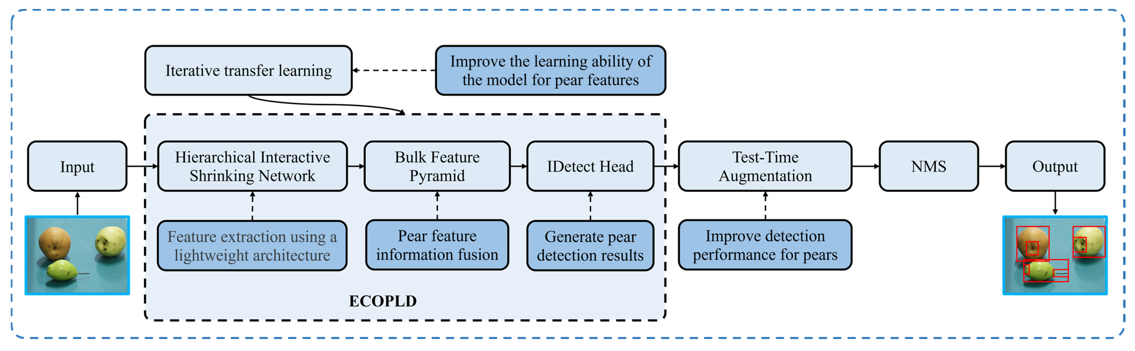
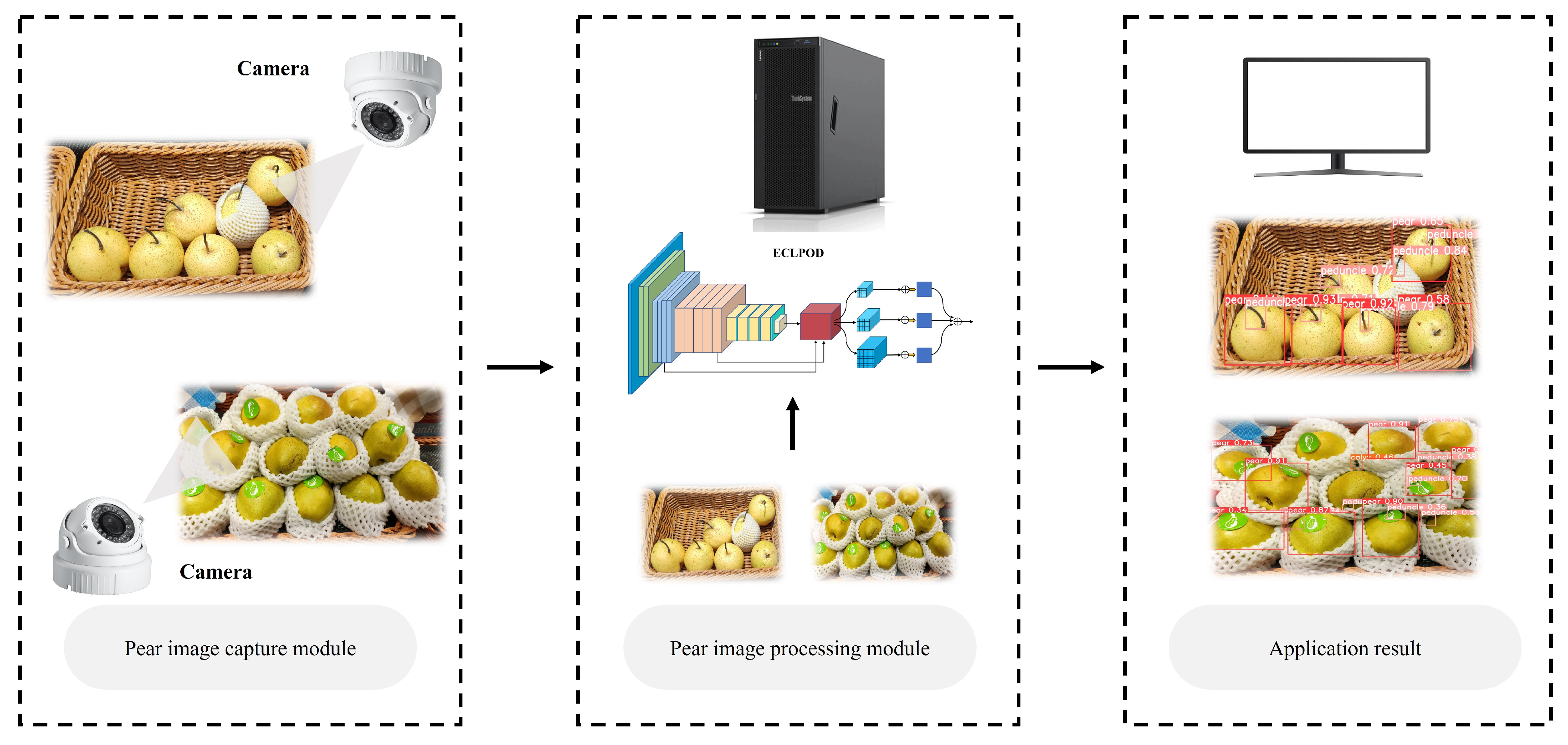
Agronomy 13 01891 g001
Figure 2. Workflow of the ECLPOD.
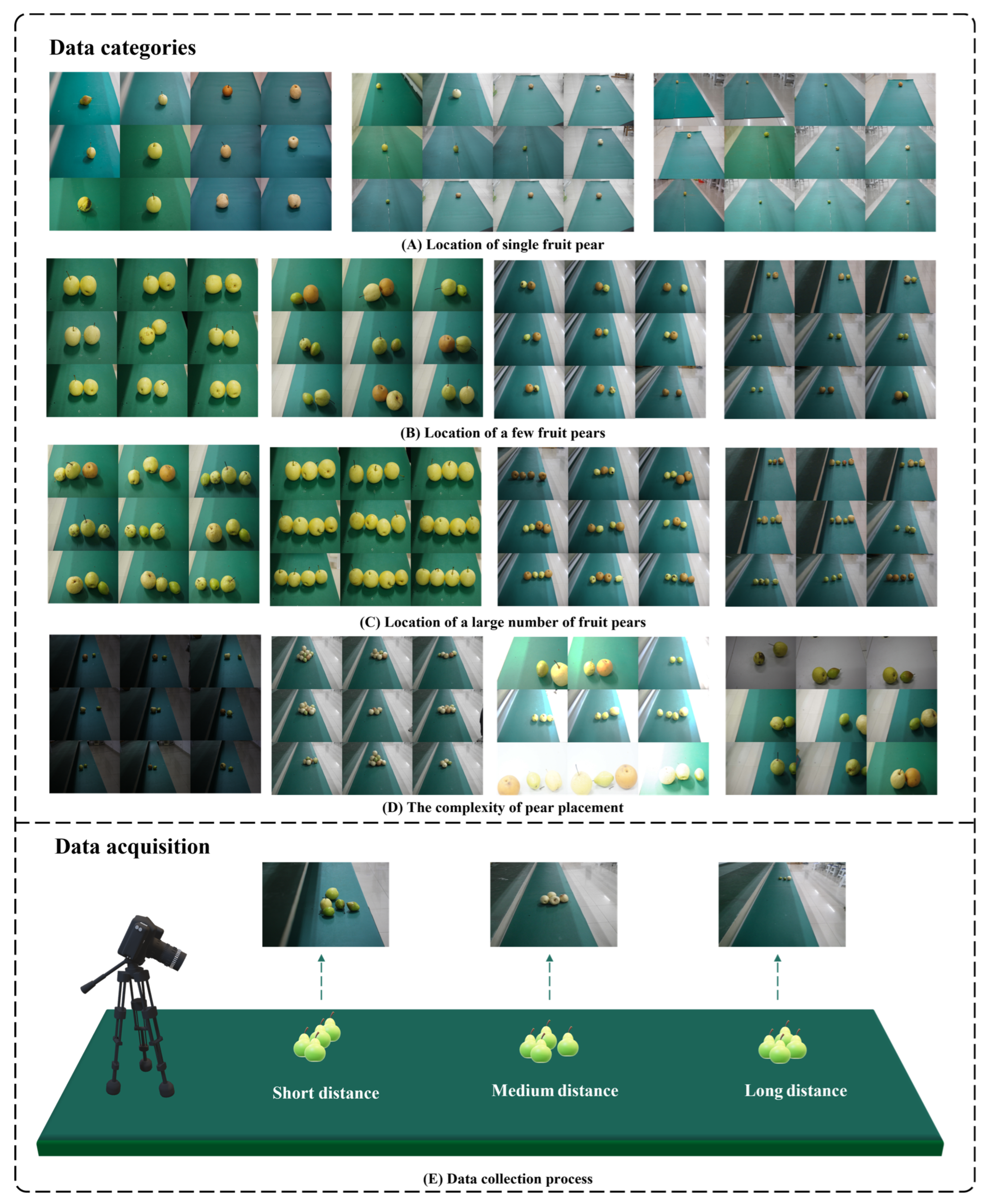
Agronomy 13 01891 g002
Figure 3. Components of experimental data and data collection methods: (A) represents the location information of a single pear in the near, medium, and far environment. (B) represents the location information of a small number of pears in the near, medium, and far environment. (C) represents the location information of multiple pears in near, medium, and far environments. (D) represents pear position information in a dark environment, an environment with more shade, an environment with strong light, and an environment with focus deviation. (E) represents the data acquisition process for the dataset.
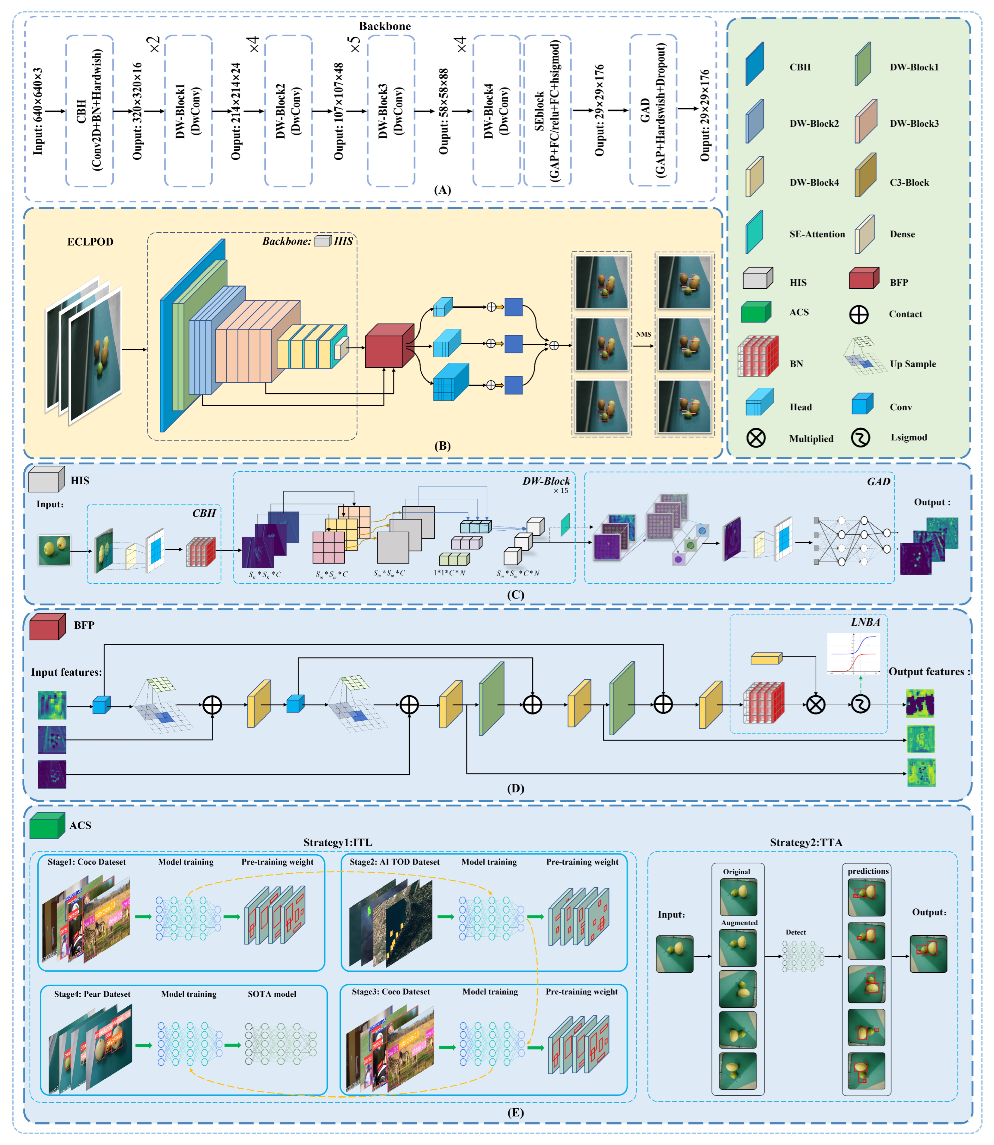
Agronomy 13 01891 g003
Figure 4. Structure of the ECLPOD: (A) The parameter transfer process of the network’s backbone. (B) The main structure of the ECLPOD. (C) The structure of the HISNet. (D) The main structure of the BFP module. (E) The ACS policies are ITL and TTA.
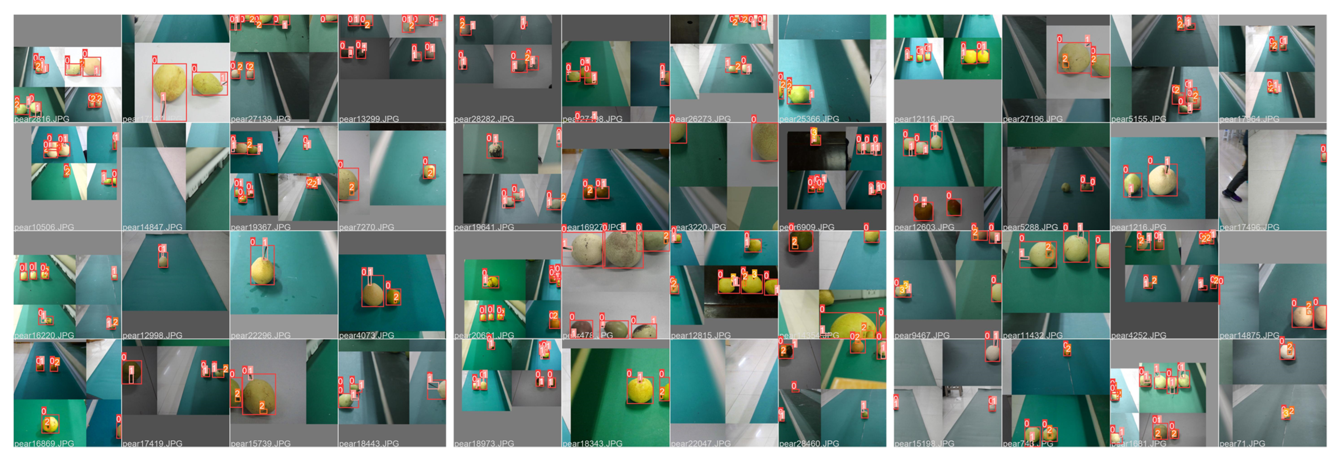
Agronomy 13 01891 g004
Figure 5. Data enhancement of pictures during training. The meanings of the numbers in the boxes in the pictures are as follows: 0 represents pear, 1 represents fruit stalk, 2 represents fruit calyx, and 3 represents defect.
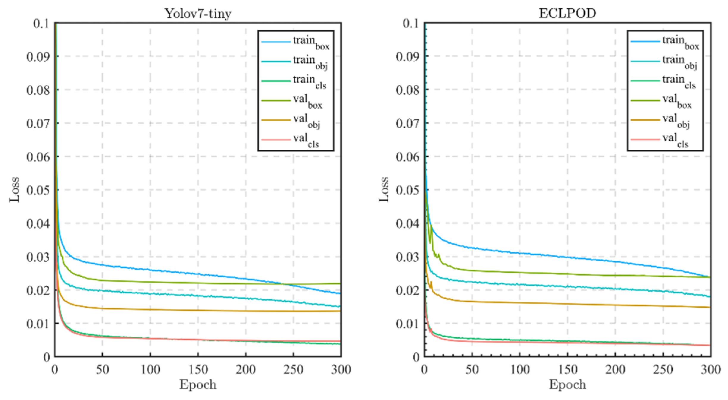
Agronomy 13 01891 g005
Figure 6. Loss changes during training and verification.
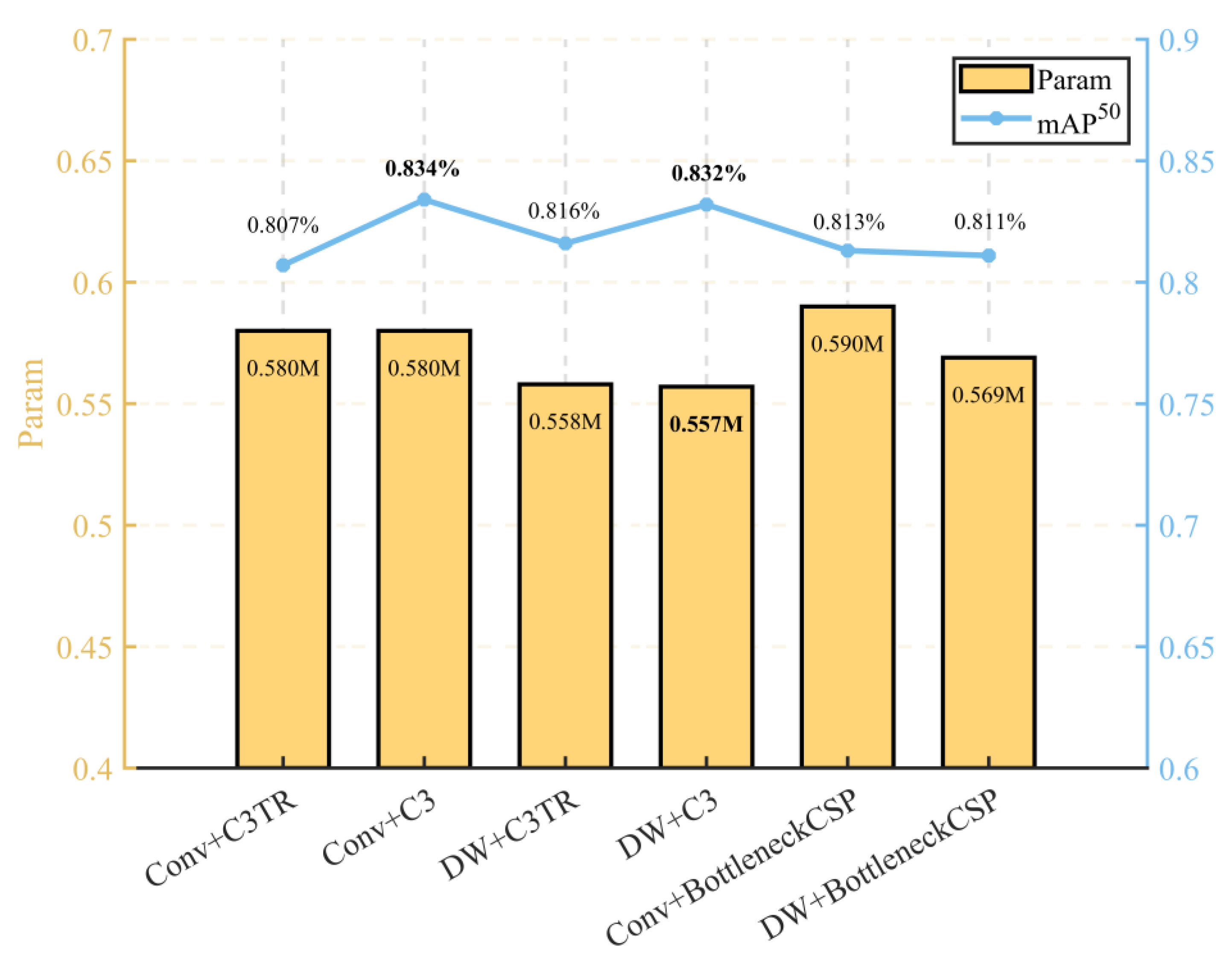
Agronomy 13 01891 g006
Figure 7. Analysis of the effectiveness of DW block and C3.
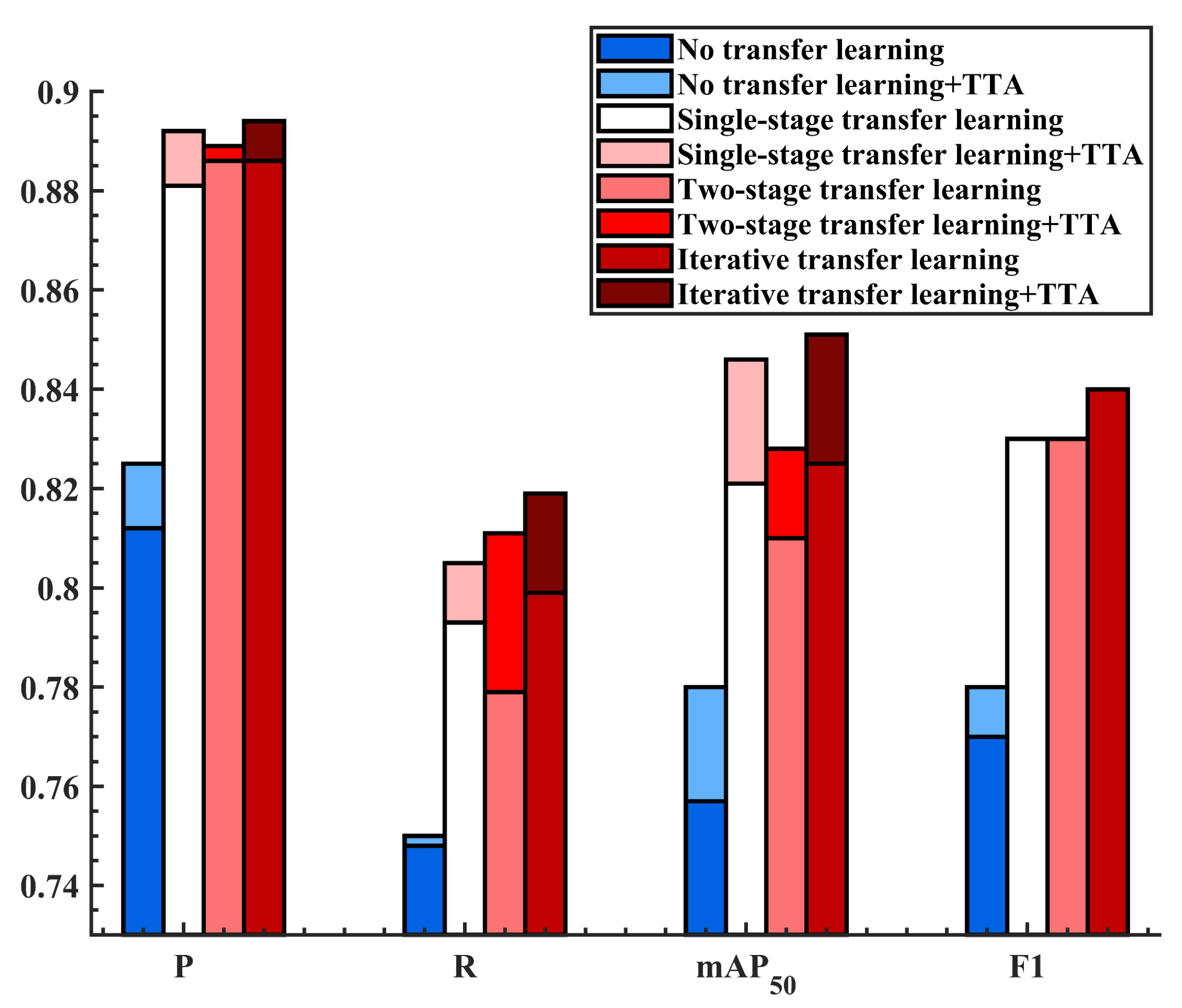
Agronomy 13 01891 g007
Figure 8. Comparison of different learning strategies.
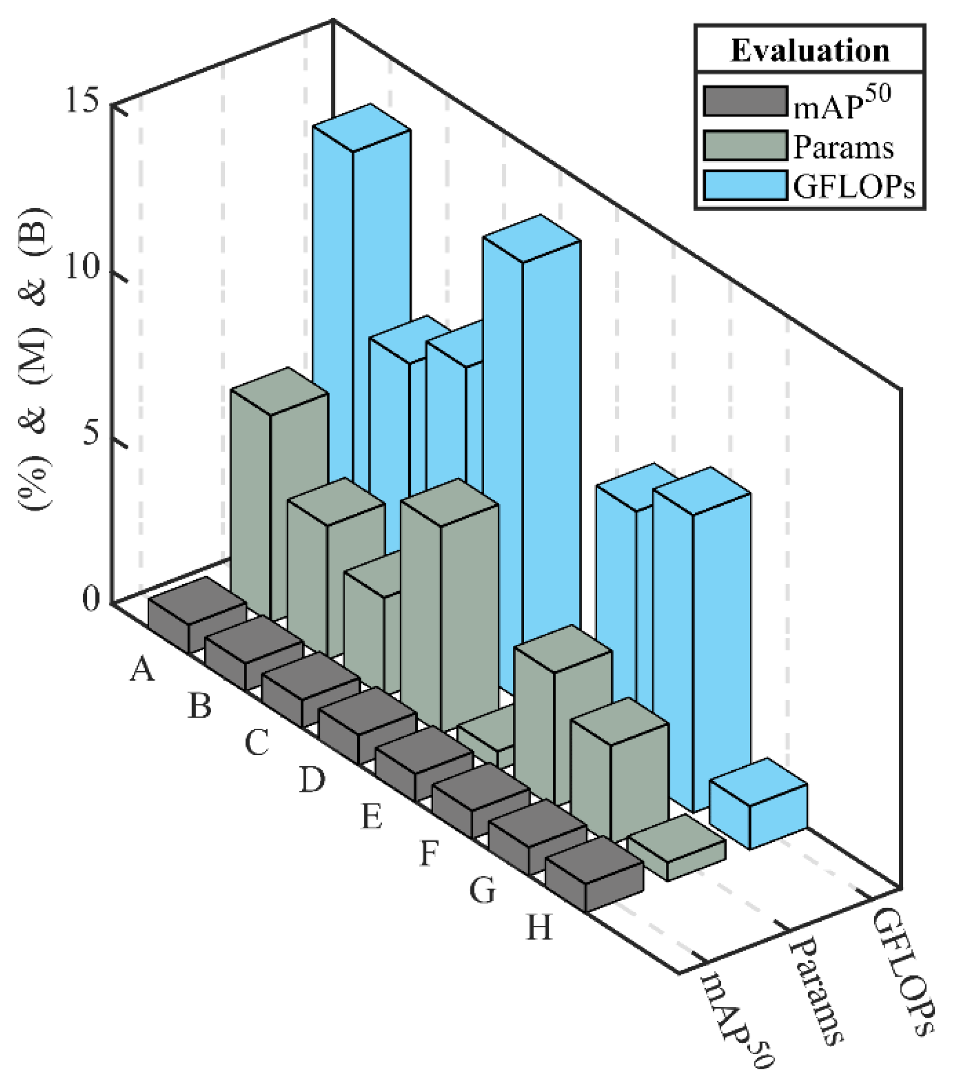
Agronomy 13 01891 g008
Figure 9. ECLPOD single ablation experiment: group A is the experimental result of YOLOv7-tiny; groups B (A + HISNet), C (A + BFP), and D (A + ACS) are the unidirectional ablation results; groups E (B + BFP), F (B + ACS), and G (C + ACS) are the bidirectional ablation results; and group H is the experimental result of the ECLPOD.
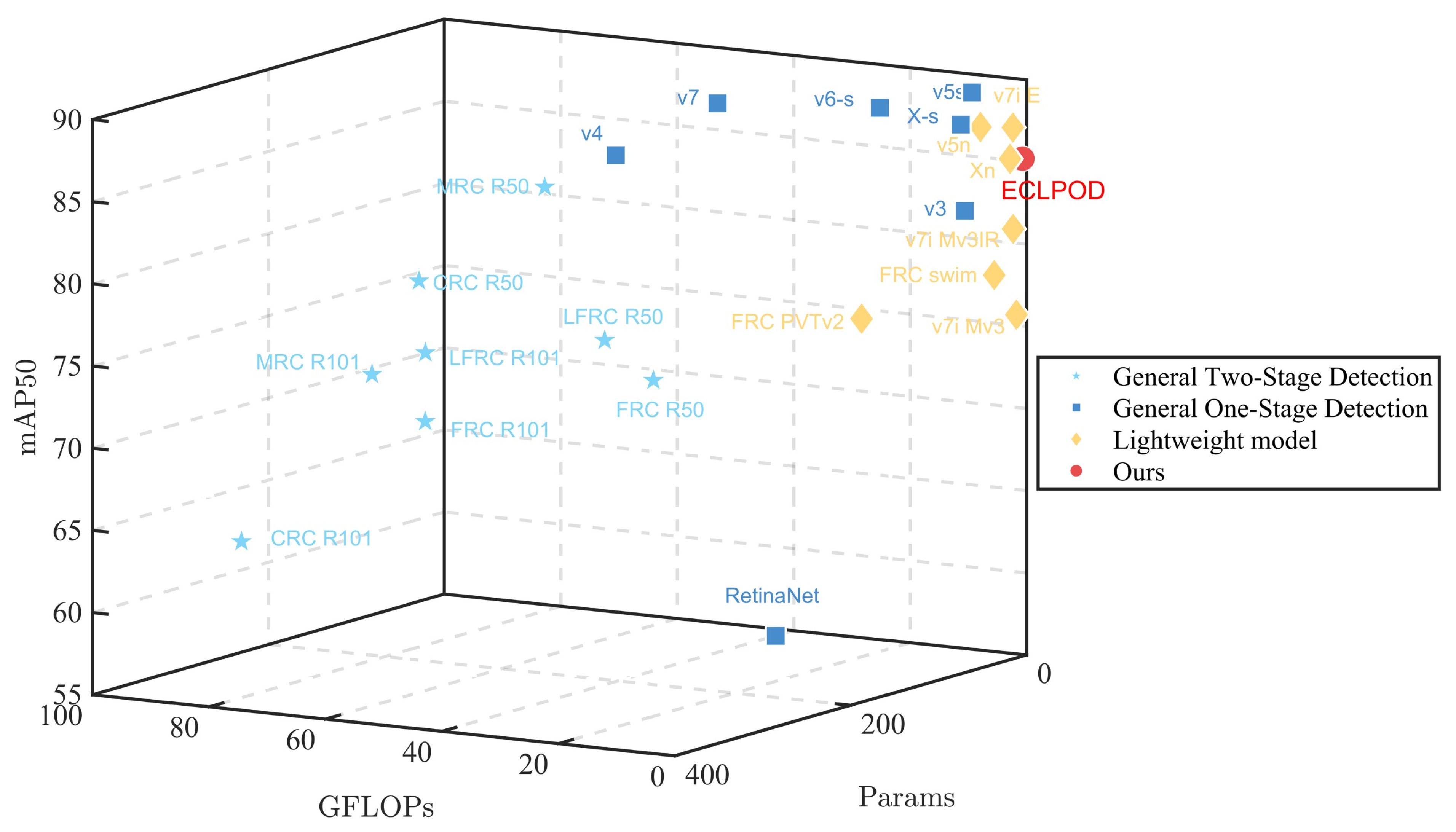
Agronomy 13 01891 g009
Figure 10. Comparison between different models and the ECLPOD. Network interpretation: FRC stands for Faster R-CNN, MRC stands for Mask R-CNN, CRC stands for Cascade R-CNN, LFRC stands for LibraFaster R-CNN, RetinaNet stands for RetinaNet; and v3, v4, v5, v6, v7, and x represent YOLOv3, YOLOv4, YOLOv5, YOLOv6, YOLOv7, and YOLO-X, respectively. Backbone description: R50, R101, PVT, swin, Mv3IR, respectively represent ResNet-50, ResNet-101, the pyramid vision transformer, Swin transformer, and MobileNetv3.
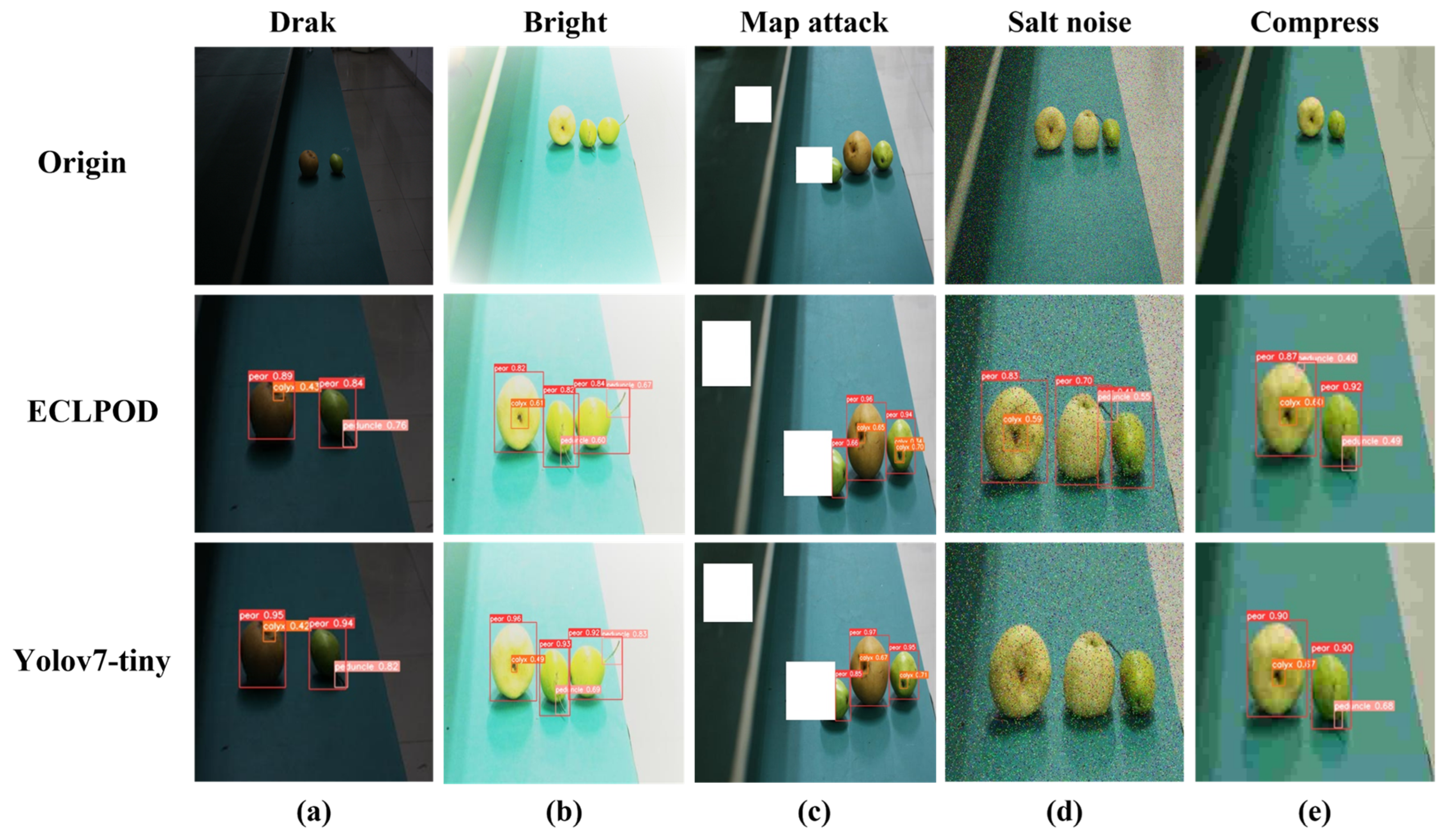
Agronomy 13 01891 g010
Figure 11. Anti-jamming comparison of the models. To facilitate the display of test results, the analysis results are enlarged. Among them, (a) is a dark environment, (b) is a light environment, (c) is subjected to texture attacks, (d) is a salt and pepper noise environment, and (e) is an image compression environment.
Agronomy 13 01891 g011
Figure 12. Generalization Performance Analysis.
Agronomy 13 01891 g012
Figure 13. Detection of different defect situations.
Agronomy 13 01891 g013
Table 1. Abbreviations table.
AbbreviationExplanation
ECLPODExtremely Compressed Lightweight Model for Pear Object Detection
HISNetHierarchical Interactive Shrinking Network
BFPBulk Feature Pyramid
LNBALearnable Based on Normalized Attention
ACSAccuracy Compensation Strategy
ITLIterative transfer learning
TTATest Time Augmentation
Table 2. Symbol explanation table.
SymbolExplanation
y ( p 0 , c ) The value at P 0 of the c channel feature map after deep convolution.
y ( p 0 ) The value at position P 0 in the final output feature map.
R The effective receptive field area of the convolution kernel.
w ( p n , c ) The weight of depth convolution.
w ( c ) The weight of point-by-point convolution.
O C The computation of ordinary convolution.
D S C The computational amount of depth-separable convolution.
F i n The input feature map of the LNBA model.
F o u t The output feature map of the LNBA model.
B N o u t A feature normalization of input features.
W e i g h t The normalized BN layer weight.
R I B ( α ) Value of the information bottleneck.
Table 3. Overview of deep learning-based sorting methods.
YearsMethodsAdvantagesDisadvantagesDataset
2020Detection and classification of bruises on pears based on thermal images [21]The accuracy rate of pear bruise detection reached 99.25%Equipment is too complicated4371
2021Deep learning based on residual networks for automatic sorting of bananas [22]Accurate summary of banana quality gradesBananas are not targeted600
2021Waste management using an automatic sorting system for carrot fruit based on image processing techniques and improved deep neural networks [23]Carrots were graded with an accuracy of 93.9 percentThe model is simple and does not fully exploit the characteristics of the data878
2022Apple stem/calyx real-time recognition using the YOLOv5 algorithm for an automatic fruit loading system [11]Adjusting fruit posture through the fruit calyx and fruit stalk helped achieve an accuracy rate of 93.89%The application scenario is simple7660
2022Appearance quality classification method for Huangguan pear under complex backgrounds based on instance segmentation and semantic segmentation [24]Accurate identification of diseased Crown pearsThe three-stage model is too complex for practical application5562
2023An efficient classification process using supervised deep learning and robot positioning based on embedded PD-FLC [25]Real-time identification and classification of fruitsDoes not consider the occlusion of the fruit6600
2023Sorting of fresh tea leaf using deep learning and air blowing [26]It better solves the decline in recognition accuracy caused by the mixed grades of fresh tea leavesOnly the use of simple cases is considered6400
2023Application of deep learning diagnoses for multiple trait sorting in peach fruit [27]Diagnosis is possible through RGB images without the need for complex equipmentUnable to detect internal defects1512
Table 4. The number of labels in the dataset.
Dataset SettingLabels with PearsLabels with PeduncleLabels with CalyxLabels with DefectTotal LabelsLabels per Image
Train set43,14831,72215,376208792,3334.51
Val set18,49613,664654391939,6224.52
Robust set10,9376333504941422,7334.20
Table 5. Software and hardware environment settings.
Hardware
environment
CPU32 vCPU Intel(R) Xeon(R)
Platinum 8350C CPU @ 2.60 GHz
RAM43 GB
Video memory24 GB
GPUNVIDIA GeForce RTX 3090
Software
environment
OSLinux
Miniconda conda3Python 3.8.10 (ubuntu20.04)
Cuda 11.3Torch 1.9.1 + cu111
CUDNN 8005Torchaudio 0.9.1
Torchvision 0.10.1 + cu111YOLOAir-v1.0
MMCV-full 1.6.1MMdet 2.25.1
Table 6. Experimental parameter settings.
Parameter CategoryParameter NameParameter Setting
SGD optimizerInitial learning rate0.01
Weight decay5 × 10−4
Momentum0.937
Learning rate decay0.005
Input data parametersSize of input images(640,640)
Batch size32
Training epochs300
IoU threshold0.6
Table 7. Model performance comparison.
EvaluationYOLOv7-TinyECLPOD
APpear99.43(−0.02~+0.03)99.44(−0.02~+0.05)
APpeduncle93.42(−0.02~+0.05)91.23(−0.08~+0.11)
APcalyx81.11(−0.13~+0.11)78.50(−0.07~+0.14)
AP5087.10(−0.04~+0.08)83.10(−0.09~+0.15)
AP50:9558.20(−0.05~+0.09)52.72(−0.06~+0.12)
F10.840.84
FPS106112
Params(M)6.020.55
Table 8. Visual comparison of the networks.
EvaluationYOLOv7-TinyECLPOD
Input layer 1 of the networkAgronomy 13 01891 i001Agronomy 13 01891 i002
The last layer of the backboneAgronomy 13 01891 i003Agronomy 13 01891 i004
The last layer of the neckAgronomy 13 01891 i005Agronomy 13 01891 i006
The last layer of the headAgronomy 13 01891 i007Agronomy 13 01891 i008
Table 9. Comparing the HISNet with other lightweight networks.
MethodParamGFLOPsmAP50APpear
YOLOV7-tiny6.21 M13.2087.10(−0.04~+0.08)99.43(−0.01~+0.01)
+Mobilenetv3-InvertedResidual [38]4.82 M8.1180.90(−0.13~+0.11)99.42(−0.03~+0.02)
+ShuffleNet V2 [39]5.39 M9.7477.90(−0.17~+0.12)99.23(−0.02~+0.04)
+HISNet4.01 M7.8282.10(−0.08~+0.15)99.51(−0.01~+0.02)
Table 10. Comparison of the effect of attention.
MethodF1ParamGFLOPsmAP50
Without Attention0.840.557 M1.382.5(−0.07~+0.11)
+CA [40]0.830.562 M1.380.7(−0.13~+0.12)
+CBAM [41]0.830.562 M1.381.9(−0.11~+0.09)
+LNBA0.840.558 M1.383.2(−0.09~+0.07)
Table 11. Training results for different learning strategies.
MethodPRF1mAP50
No transfer learning81.2074.8077.0075.70(−0.27~+0.19)
No transfer learning (+TTA)82.5075.0078.0078.01(−0.24~+0.15)
Single-stage transfer learning88.1079.3083.0082.10(−0.16~+0.06)
Single-stage transfer learning (+TTA)89.2080.5084.6083.24(−0.14~+0.04)
Two-stage transfer learning88.6077.9083.0081.00(−0.18~+0.11)
Two-stage transfer learning (+TTA)88.9081.1082.8083.02(−0.11~+0.15)
Iterative transfer learning88.6081.4282.0083.20(−0.09~+0.15)
Iterative transfer learning (+TTA)90.1082.9083.1085.20(−0.07~+0.14)
Table 12. ECLPOD single ablation experiment.
GroupMethodF1ParamsGFLOPsmAP50
AYOLOv7-tiny0.846.2213.2087.11(−0.06~+0.11)
B+HIS0.794.017.9482.17(−0.13~+0.16)
C+BFP0.772.968.9483.41(−0.15~+0.22)
D+ACS0.856.2113.2089.22(−0.04~+0.14)
E+HIS+BFP0.820.561.3083.21(−0.06~+0.08)
F+HIS+ACS0.824.037.9483.32(−0.06~+0.13)
G+BFP+ACS0.812.968.9484.83(−0.09~+0.12)
H+HIS+BFP+ACS0.830.551.3085.20(−0.07~+0.14)
Table 13. Comparison of different models.
MethodBackbonePrecisionParam(M)GFLOPsmAP50
General Two-Stage Detection
Faster R-CNNResNet-5081.140.54156.0472.61(−0.31~+0.21)
Faster R-CNNResNet-10179.560.52283.1471.32(−0.29~+0.26)
Cascade R-CNNResNet-5083.468.94234.4778.81(−0.25~+0.17)
Cascade R-CNNResNet-10174.787.93310.5563.41(−0.43~+0.56)
Mask R-CNNResNet-5088.943.76258.2285.85(−0.18~+0.11)
Mask R-CNNResNet-10180.262.65329.5474.84(−0.24~+0.31)
LibraFaster R-CNNResNet-5082.041.1207.7375.82(−0.22~+0.19)
LibraFaster R-CNNResNet-10181.560.39283.875.57(−0.18~+0.26)
General One-Stage Detection
RetinaNetResNet-1860.319.68155.1157.89(−1.31~+0.87)
YOLOv3DarkNet-5389.38.6712.9081.91(−0.15~+0.13)
YOLOv4CSPDarknet-5389.952.51119.7085.32(−0.11~+0.04)
YOLOv5-sCSPDarknet-5391.77.0215.8089.24(−0.07~+0.04)
YOLOX-sCSPDarknet89.98.0521.8086.36(−0.08~+0.14)
YOLOv6-sEfficientrep90.818.445.1088.37(−0.12~+0.03)
YOLOv7E-ElAN91.937.2105.2088.87(−0.04~+0.08)
YOLOv7-tinyE-ElAN91.26.0113.0087.12(−0.07~+0.11)
Lightweight model
Faster R-CNNSwim85.24.229.1278.10(−0.3~+0.04)
Faster R-CNNPVTv284.36.8142.8977.41(−0.15~+0.18)
YOLOv5-nCSPDarknet-5389.41.764.1085.17(−0.11~+0.03)
YOLOX-nCSPDarknet89.72.025.7085.22(−0.08~+0.11)
YOLOv7-tinyMobilenetv3-bench81.21.42.4075.71(−0.21~+0.16)
YOLOv7-tinyMobilenetv3-InvertedResidual88.31.92.8080.91(−0.13~+0.11)
Ours
ECLPODHISNet90.10.551.3085.20(−0.07~+0.14)
Table 14. Comparison of test results.
Experimental
Method
Detection Result
YOLOv7-tiny
(Mobilenetv3)
Agronomy 13 01891 i009Agronomy 13 01891 i010Agronomy 13 01891 i011
YOLOX-nAgronomy 13 01891 i012Agronomy 13 01891 i013Agronomy 13 01891 i014
YOLOv5nAgronomy 13 01891 i015Agronomy 13 01891 i016Agronomy 13 01891 i017
ECLPODAgronomy 13 01891 i018
(a)
Agronomy 13 01891 i019
(b)
Agronomy 13 01891 i020
(c)
Table 15. Experimental results of one-way ANOVA.
NoFp-ValueF Crit
Table 91747.944.15 × 10−163.490295
Table 1023,482.597.16 × 10−233.490295
Table 119.9967360.000122.946685
Table 121619.5059.87 × 10−243.4668
Table 138.6793244.17 × −10−52.708186
Disclaimer/Publisher’s Note: The statements, opinions and data contained in all publications are solely those of the individual author(s) and contributor(s) and not of MDPI and/or the editor(s). MDPI and/or the editor(s) disclaim responsibility for any injury to people or property resulting from any ideas, methods, instructions or products referred to in the content.

