Research and Validation of Potato Late Blight Detection Method Based on Deep Learning

Abstract

Late blight, caused by phytophthora infestans, is a devastating disease in potato production. In severe cases, this can lead to potato crop failure. To rapidly detect potato late blight, in this study, a deep learning model was developed to discriminate the degree of potato leaf diseases with high recognition accuracy and a fast inference speed. It constructed a total of seven categories of potato leaf disease datasets in single and complex backgrounds, which were augmented using data enhancement method increase to increase the number of images to 7039. In this study, the performance of the pre-trained model for fine-grained classification of potato leaf diseases was evaluated comprehensively in terms of accuracy, inference speed, and the number of parameters. The ShuffleNetV2 2× model with better generalization ability and faster inference speed was selected and improved. Three improvement strategies were proposed: introducing an attention module, reducing the depth of the network, and reducing the number of 1 × 1 convolutions. Their effects on the performance of the underlying model were explored through experiments, and the best form of improvement was determined. The loss function of the improved model converged to 0.36. This was compared to the base model, which was reduced by 34.5%. In the meantime, the improved model reduced the number of parameters, FLOPs, and model size by approximately 23%, increased classification accuracy by 0.85%, and improved CPU inference speed by 25%. Deploying the improved model to the embedded device, the overall classification precision was 94%, and the average time taken to detect a single image was 3.27 s. The method provided critical technical support for the automatic identification of potato late blight.

1. Introduction

According to the United Nations Food and Agriculture Organization (FAO) statistics, 157 countries around the world grow potato, which has a total planting area of 19.46 million hm² and an annual yield of 370 million tons [1]. China has become the world’s largest potato producer; its planting area and yield are ranked first in the world [2]. Potato late blight is one of the important factors limiting its yield level. Therefore, developing a model for detecting potato late blight can overcome the limitations of manual feature extraction and enable early monitoring and prevention of the disease. This approach has great practical significance in enhancing potato yields, reducing production costs, and increasing revenue.

Deep learning networks offer exceptional speed and accuracy in recognition tasks, demonstrating strong robustness and generalization capabilities. By circumventing the need for manual feature extraction and intricate feature segmentation operations, deep learning minimizes the risk of misclassifying or omitting crucial target features during pre-feature sampling [3]. Consequently, deep learning has been widely used in various domains, including medical disease diagnosis [4,5,6], agricultural product detection [7,8,9,10], protein cell localization [11], etc.

In the realm of crop disease detection, Mohanty et al. [12] employed Convolutional Neural Networks (CNN) to train a system capable of automatically diagnosing plant diseases. Their study encompassed 54,306 images of healthy and diseased plant leaves. Both the AlexNet and GoogLeNet frameworks were utilized, along with transfer learning techniques, to handle the dataset and mitigate the issue of overfitting. The system achieved an accuracy of 99.35%. However, it is worth noting that this accuracy diminishes when tested on images captured under conditions different from those in the training set. Huang et al. [13] developed a rice panicle blast detection system using the GoogLeNet model and introduced two data enhancement strategies. The first strategy involved randomly discarding one band image, while the second strategy entailed randomly adjusting the average spectral image brightness through panning. These strategies aimed to augment the training data size, prevent overfitting, improve the model’s generalization performance, and reduce the impact of natural light on its performance. Rahman et al. [14] proposed a lightweight two-stage CNN network designed for identifying 14 distinct types of pests in rice. Their research focused on streamlining the network structure to enhance training speed. To validate the effectiveness of their proposed network, they conducted a comparative analysis against established models, such as VGG-16, Inception V3, and MobileNet-V2, employing fine-tuning or transfer learning techniques. Barman et al. [15] developed a CNN network specifically designed for the identification of late blight, early blight, and healthy leaves in potatoes. The network was evaluated using both the original and enhanced datasets. The results demonstrated that the network exhibited superior performance in identifying the enhanced dataset while avoiding overfitting issues. Furthermore, the researchers successfully implemented the network into an Android application, enabling real-time detection of potato leaf diseases. Chen et al. [16] employed migration learning to leverage a pre-trained DenseNet on a dataset of rice diseases, effectively extracting disease features. These features were then integrated and classified using the Inception module. To enhance the learning capability of minor disease features, the network incorporated a focal loss function in place of the original cross-entropy loss function. As a result, their method achieved a prediction accuracy of 90.14% for five common pests and diseases affecting rice. Suarez et al. [17] used Convolutional Neural Networks (CNNs) and support vector machines (SVMs) for the early detection of late blight on potatoes and showed that the CNN model performed well for the diagnostic classification of potato leaf diseases, with the highest accuracy of 93.2%. Eser [18] integrated Faster R-CNN and GoogLeNet models to successfully discriminate between three diseases affecting pepper and potato leaves. Faster R-CNN was employed for extracting image features, while GoogLeNet was utilized for disease classification. The combined approach achieved an average classification accuracy of 95.6% and a recall rate of 96.4%. The above studies demonstrate the feasibility and effectiveness of deep learning for crop disease recognition and classification, but the models with publicly available datasets are less effective in the actual field environment and can be affected by factors, such as lighting, debris, and leaf shading. In this study, we proposed to construct image datasets with different growth periods, angles, lighting conditions, and background changes to ensure the robustness of the model.

The deployment of deep learning-based disease detection models on mobile devices is crucial for achieving automated monitoring and early warning of crop diseases. However, such models demand high hardware performance, while mobile phones and ARM devices are constrained by limited memory and computational power. Consequently, this limitation adversely affects the model’s accuracy and inference speed. To address these challenges, it becomes necessary to strike a balance between the performance and size of the detection model, ensuring seamless collaboration between software and hardware components. To address the above issues, this study proposed a deep learning-based model for discerning the severity of potato late blight. The research objectives of this study are as follows:

(1)

To attain fine-grained disease classification by leveraging classical lightweight classification networks. To evaluate the performance of each model based on classification accuracy and model complexity to identify the model that exhibits the highest generalization ability, which will serve as the foundation for further research.

(2)

To optimize the chosen base model by reducing the number of model parameters and increasing the speed of inference, while ensuring that classification accuracy is not compromised.

(3)

To evaluate the feasibility and effectiveness of running the model on hardware, the optimized model was deployed on an embedded device.

2. Materials and Methods

2.1. Image Data Acquisition

To address the challenge of distinguishing between late blight and early blight in the early stages of potato disease, the Potato Leaf Disease Dataset (PLDD) was created. It included images of both diseased and healthy leaves. The dataset utilized images of late blight and early blight from the Plant Village dataset [19] and healthy leaves from the AI Challenger 2018 dataset (https://challenger.ai/dataset/pdd2018, accessed on 19 May 2023). These images were captured under consistent conditions, including the same shooting distance, lighting conditions, and environmental background. This ensured that the leaves and their disease spots stood out prominently from the background. To enhance the dataset’s diversity and reliability, additional potato disease images in natural backgrounds were sourced from the Kaggle website (https://www.kaggle.com/datasets/hassanikram/my-dataset, accessed on 19 May 2023). To ensure high image quality, any images with poor clarity or noticeable watermarks were manually eliminated. Furthermore, images containing multiple leaves were cropped to maintain the dataset’s focus on single leaf and single disease characteristics. An example of the leaf images featured in PLDD can be seen in Figure 1.

2.2. Images Annotation

In deep learning, the classification network employs supervised learning, which necessitates a substantial quantity of labeled data to train the model. Consequently, it is essential to establish appropriate labels for the PLDD data in the classification network. To ensure objectivity in the classification process, this study adhered to the national field grading standards for late blight and early blight of potatoes [20], wherein the severity of the disease was determined by the percentage of the affected area. Therefore, each image in the dataset required separate labeling for the entire leaf and the area affected by the disease.

(1)

Leaf annotation

The Labelme software was utilized to annotate the entire leaf area of the PLDD image. In this labeling process, the whole leaf area was marked in red, while the background was marked in black. An example of the PLDD data after leaf labeling can be seen in Figure 2.

(2)

Disease spot annotation

From Figure 1, it can be observed that the severity of diseases in the PLDD images varies. In the case of late blight, the leaves exhibit irregular brown-green patches on the surface during the advanced stage of the disease. In a humid environment, white mildew may appear on the leaves, while under dry conditions, the entire leaf can wither and shrink. On the other hand, in the case of early blight infection, the disease spots initially manifest as scattered brown circular patches, gradually enlarging to become nearly circular in shape. The disease spots display distinct concentric rings and may exhibit a yellow halo around the outer edge. Severe infections can lead to localized necrosis of the leaves. Due to variations in the progression of the disease across different leaves, the locations, quantities, and sizes of the disease spots are highly random. Additionally, with a dataset comprising nearly ten thousand images, manual annotation of the disease spots presents a significant challenge. Given the clear color distinction between healthy green leaf surfaces and disease spots, this study considers utilizing the ExG vegetation index and traditional image processing methods to differentiate the disease spots. The process for extraction the disease areas is illustrated in Figure 3, the specific steps are as follows.

• Production of leaf foreground image: the label image obtained after the labeling of the leaf will be converted into a binary image to obtain a mask image of the leaf, and then it will be bit-operated with the original image to obtain an image containing only the foreground of the leaf.
• Extraction of the super green features of the image: calculation of the vegetation index EXG of the foreground image of the leaf, as well as the transformation of its color space from three channels to a single channel to obtain a greyscale image.
• Acquisition of non-spotted areas: set the gray value of the pixels with a gray value between 30 and 200 to 0 and the rest to 255. The image is changed from a grey-scale image to a binary image with a black background and diseased areas in white and non-diseased areas in black.
• Get the diseased area: the non-diseased area and the leaf mask image are bit-operated, and then morphological operations are performed to eliminate the fine outline of the leaf edge to obtain a complete mask image of the diseased area.
• Creating a labeled image of the spot: iterate through all the pixels of the image, reassigning those with a gray value of 255 for all three channels—r, g, and b. Pixels with a gray value of 255 are reassigned.

By utilizing the annotations of the leaves and disease spots, the pixel count and corresponding ratios are calculated. This enables the determination of the disease severity level based on the field grading standard. Therefore, in this study, we initially considered a slight modification to the classification criteria, aiming to reduce the sample size by decreasing the granularity of disease classification. The modified classification criteria and the number of images for each disease type are presented in

Table 1. The statistics of the number of images contained in each disease type, classified according to the disease classification criteria.

Percentage of Spots (%)	Disease Level	Number of Single Background Images			Number of Single Background Images
		Early Blight	Late Blight	Healthy	Early Blight	Late Blight	Healthy
<1	Healthy	/	/	1582	/	/	50
1~15	Level 1	613	462	/	54	51	/
15~40	Level 2	341	428	/	45	89	/
>40	Level 3	46	110	/	12	60	/

Note: “/” in the table means there is no image of this category.

. The results indicate that there are a relatively small number of images at disease level 3. To address this issue, the dataset was further expanded through data augmentation.

2.3. Image Data Expansion

Data augmentation is a technique used to address the issue of insufficient training data or class imbalance in the dataset [21]. In this study, various image enhancement techniques, such as flipping, HSV enhancement, brightness adjustment, and adding shadows, were used. As a result, the total number of PLDD images was increased to 7039, which included 1720 healthy leaf images and 5319 diseased leaf images. The diseased leaf images were further divided into 3 levels each of early blight and late blight, resulting in 881 early blight level 1 images, 889 early blight level 2 images, 850 early blight level 3 images, 884 late blight level 1 images, 922 late blight level 2 images, and 893 late blight level 3 images, and the number of healthy leaf images was about twice as many as the remaining 6 types of images.

In this study, the expanded PLDD dataset was divided into three sets: the training set, validation set, and test set, with a ratio of 6:2:2. The training set was used to train the model, the validation set was employed for hyperparameter tuning, and the test set was utilized to evaluate the model’s generalization performance. To ensure proportional distribution across the three sets, the images were randomly sampled and categorized accordingly. This process ensured that each set contained both single background and natural background images. Consequently, the three divided datasets consisted of 4206, 1418, and 1415 images, respectively.

2.4. Methodologies

2.4.1. ShuffleNetV2

In 2018, Ma et al. [22] introduced the ShuffleNetV2 network, an improvement upon ShuffleNetV1, based on four efficient network design principles. ShuffleNetV2 incorporates a channel-splitting approach. Initially, the channel dimension of the input feature map is evenly divided into two branches. The left branch undergoes equal mapping, while the right branch undergoes successive convolutions with 1 × 1, 3 × 3 depth separable, and 1 × 1 convolutions. These operations ensure that the input and output channels remain the same. Subsequently, the outputs of the two branches are fused together using a concatenation operation, allowing for information exchange. Additionally, when the convolution step is 2, indicating spatial down sampling, the channel splitting operation is removed to double the output dimension. The fundamental unit of the ShuffleNetV2 network is depicted in Figure 4a,b.

The ShuffleNetV2 network architecture, including its specifications, can be found in

Table 2. The structure of ShuffNetV2.

Layer	Output Size	Kernel Size	Stride	Repeats	Number of Output Channels
					0.5×	1×	1.5×	2×
Image	224 × 224				3	3	3	3
Conv1	112 × 112	3 × 3	2	1	24	24	24	24
MaxPool	56 × 56	3 × 3	2
Stage 2	28 × 28		2	1	48	116	176	244
	28 × 28		1	3
Stage 3	14 × 14		2	1	96	232	352	488
	14 × 14		1	7
Stage 4	7 × 7		2	1	192	464	704	976
	7 × 7		1	3
Conv 5	7 × 7	1 × 1	1	1	1024	1024	1024	2048
Global Pool	1 × 1	1 × 1
FC

. The network primarily consists of a stack of basic units, alternating between Stride = 1 and Stride = 2 units. In each stage, there is one Stride = 2 unit, followed by 3, 7, and 3 repetitions of Stride = 1 units, respectively. In this research, the 2× version of ShuffleNetV2 is employed, where the numbers of output channels for each stage are 244, 488, and 976, respectively. Subsequently, a 5 × 5 convolutional layer is applied to increase the number of channels to 2048.

2.4.2. Attention Module

(1)

SE Module

The SE (Squeeze-and-Excitation) module, introduced by Hu et al. [23], incorporates three key steps: Squeeze, Excitation, and Scale (re-weighted feature map). The module operates as follows. Firstly, in the Squeeze step, global average pooling is applied to the input features, resulting in a compression of the spatial dimension. Next, in the Excitation step, the globally compressed features are connected twice through fully connected layers to capture the nonlinear relationships between channels. The first fully connected layer reduces the dimensionality of the features, while the second fully connected layer restores the feature dimensionality. A Sigmoid function is then utilized to restrict the weights of each channel within the range of 0 to 1. Lastly, in the Scale step, the input feature map is multiplied by the channel weights, completing the recalibration of feature maps across different channels.

(2)

CBAM Module

The CBAM (Convolutional Block Attention Module) attention mechanism is a fusion of channel and spatial attention modules, designed for enhancing feature representation [24]. It operates in a sequential manner, applying the channel attention module, followed by the spatial attention module. In the channel attention module, the spatial information of the feature map is first aggregated using both maximum pooling and average pooling operations. The resulting one-dimensional vectors are then fed into a shared layer, consisting of a multilayer perceptron and an implicit layer. The outputs from the shared layer are summed, and the channel attention mapping, denoted as Mc, is obtained using the Sigmoid function. As with the SE module, a channel dimensionality reduction is performed using the shared layer to reduce the parameter scale. Mc is multiplied element-wise with the input feature map F to obtain the intermediate feature map F′. Next, in the spatial attention module, average pooling and maximum pooling operations are applied along the channel axis to the intermediate feature map F′. The outputs from these operations are concatenated to generate a valid feature descriptor. A convolutional layer is then employed to generate the spatial attention map, denoted as Ms. Finally, Ms is multiplied element-wise with the intermediate feature map F’ to obtain the output feature map F″. This sequential application of the channel and spatial attention modules effectively enhances the representation of the feature map.

(3)

ECA Module

Wang et al. [25] proposed the ECA module as a solution to the challenge of balancing model performance and complexity. While the SE module can enhance model performance, it comes with a higher computational cost. In contrast, the ECA module only has a small number of parameters, but it can still significantly improve performance. The ECA module achieves this by utilizing a local cross-channel interaction strategy that does not require dimensionality reduction. Instead, it considers each channel and its k nearest neighbors, implementing cross-channel interaction efficiently through a one-dimensional convolution with a kernel size of k. The kernel size k determines the range of cross-channel interaction and avoids unnecessary information exchange for all channels. To avoid the need for manual tuning of k through cross-validation, the ECA module uses a nonlinear function of adaptive mapping, based on the channel dimension. As a result, the convolutional kernel size k is proportional to the number of channels, ensuring optimal performance without sacrificing efficiency.

The structure of the ECA module is illustrated in Figure 5. It applies a one-dimensional convolution with a kernel size of k to the features obtained after global average pooling. The ECA module effectively replaces the two fully connected layers in the SE module with a one-dimensional convolution. As a result, the ECA module significantly reduces the number of parameters and computational complexity [26].

Considering that the three aforementioned attention modules can be plug-and-play and can be flexibly introduced into different positions within the network, this study evaluated the impact of the type, position, and number of attention modules on the performance of the basic model. In this study, three different positions for introducing attention modules were designed for ShuffleNetV2 units with Stride = 1 and Stride = 2, resulting in the creation of three novel ShuffleNetV2 units, referred to as Shuffle-Attention modules. The structures are depicted in Figure 6 below. For simplicity, only the Shuffle-Attention module with Stride = 1 is presented in the figure. Among these modules, the Shuffle-Attention-A module places the attention module after the 1 × 1 convolution. In the Shuffle-Attention-B module, a shortcut branch is introduced to the original right branch, and its attention module is placed within the main branch of the right branch after the 1 × 1 convolution. The key difference between Shuffle-Attention-B and Shuffle-Attention-A modules is the introduction of a residual connection in the former. On the other hand, the Shuffle-Attention-C module integrates the attention module into the channel mixing operation following the washout process. This setup aims to investigate the impact of attention modules at different positions within the ShuffleNetV2 unit. Additionally, this research explores the effect of the number of attention modules on the model’s performance. Initially, the attention module is inserted into the ShuffleNetV2 unit with step distances of 2 and 1 in Stage 2, Stage 3, and Stage 4. Then, each stage sequentially adds an attention module. To control the increase in parameter count associated with attention modules, this study adopts an introduction strategy that progresses from “shallow” to “deep”. Finally, while ensuring consistent positions and numbers of attention modules, the performance enhancements brought about by the SE, CBAM, and ECA modules are compared and evaluated.

2.4.3. Reduce Network Depth

The original ShuffleNetV2 network consists of numerous layers and exhibits excellent classification performance for large datasets, such as ImageNet. However, in this study, the classification task focuses on only seven types of images, which is relatively straightforward and does not necessitate a deep model. Consequently, this study explores the possibility of reducing the number of stacked units of Stride = 1 in each stage to decrease the network’s depth. In this study, the performance impact of reducing the stacking times in a single stage and simultaneously reducing the stacking times in multiple stages was compared and evaluated.

2.4.4. Reduce the 1 × 1 Convolutions

Within the ShuffleNetV2 unit, the 1 × 1 convolution at the end of the main branch does not serve as channel adjustment and fails to facilitate cross-channel information interaction. Instead, it merely increases the network depth, leading to an escalation in parameter count and computational complexity. To address this, the study explored the possibility of removing the terminal point convolution from certain units. The removal of the 1 × 1 convolution at the end of the right branch in units with a stride of 2 within each stage, as well as the 1 × 1 convolution at the end of the right branch in the last unit with a stride of 1, was implemented. Furthermore, the deep point convolution was progressively removed at each stage to compare its influence on the model’s performance.

2.4.5. Experimental Environment

The improved series of algorithms in this research were built in the Pycharm frame-work, and the software training environment configuration for the comparison experiments is shown in

Table 3. Experimental environment.

Configuration	Parameter
CPU	11th Gen Intel(R) Core(TM) i7-11800H @ 2.30 GHz
GPU	NVIDIA GeForce RTX 3050 Ti
Programming language	Python 3.7
Deep learning framework	Tensorflow2.0
Operating system	Windows 11

.

2.5. Evaluation of Model Performance

This research aimed to achieve an accurate classification of potato diseases at a fine-grained level. Therefore, the classification accuracy of the model is used to evaluate its generalization performance. Subsequently, the classification model needs to be deployed on embedded devices that have limited size and computing power as compared to computers or servers. Thus, this study considered model complexity as a comprehensive evaluation criterion for the performance of the classification model.

(1)

Accuracy evaluation index

In addition to utilizing classification accuracy as a metric to assess the overall classification performance of the model on the entire dataset, this study also incorporates precision, recall and F1-score for further evaluation. The calculation of accuracy, precision, recall and F1-score are presented in Formulas (1), (2), (3), and (4), respectively.

$$Accuracy=\frac{TP+TN}{T{P}_{}+FP+TN+F{N}_{}}\times 100\%$$

(1)

$$Precision=\frac{T{P}_{}}{T{P}_{}+F{P}_{}}\times 100\%$$

(2)

$$Recall=\frac{T{P}_{}}{T{P}_{}+FN}\times 100\%$$

(3)

$$F1-score=\frac{2\times Precision\times Recall}{Precision+Recall}\times 100\%$$

(4)

where: TP, FP, TN, and FN represent the number of true positive samples, false positive samples, true negative samples, and false negative samples, respectively.

(2)

Complexity evaluation index

Time complexity and space complexity are two crucial indicators used to assess the complexity of an algorithm. In deep learning models, the time complexity of a model is typically measured in terms of FLoating-point Operations Per Second (FLOPs). On the other hand, the space complexity of a model is often quantified by the number of parameters it possesses. It is worth noting that FLOPs are an indirect measure of the model’s operational speed, since factors, such as memory access cost (MAC) and other operations, also significantly occupy the overall runtime. Furthermore, the time required for inference can differ, depending on whether the model is executed on a CPU or GPU. To address this, this research conducts predictions on 500 images of size 224 × 224 using both CPU and GPU and calculates the average runtime as the model’s inference time.

3. Results and Discussion

3.1. Base Model Performance Comparison

The current prevalent lightweight backbone networks include the ShuffleNet series [27], MobileNet series [28,29,30], Ghostnet [31], and SqueezeNet [32], among others. This study conducted a comparative analysis of the classification performance of these aforementioned lightweight network models on the PLDD dataset. Multiple indicators, such as classification accuracy and model complexity, were utilized to comprehensively evaluate the performance of each model. Subsequently, the network that demonstrated the best performance was selected as the fundamental model for this chapter. The accuracy change curves for the training set and validation set of each classification network are depicted in Figure 7, while the performance index results of each network on the test set are presented in

Table 4. The performance metric results for each model on the test set.

Model	Accuracy (%)	Parameters (106)	FLOPs (109)	Model Size (MB)	Infer Time (ms)
					GPU	CPU
0.25 MobileNetV1	89.62	0.22	0.08	1.04	13.23	24.56
0.5 MobileNetV1	93.43	0.83	0.30	3.37	19.13	31.67
0.75 MobileNetV1	93.50	1.84	0.66	7.21	21.86	32.96
1.0 MobileNetV1	93.50	3.24	1.15	12.54	21.97	34.09
0.5 MobileNetV2	91.88	0.50	0.18	2.26	25.08	36.82
0.75 MobileNetV2	93.64	1.07	0.40	4.45	25.25	38.53
1.0 MobileNetV2	94.14	1.85	0.57	7.41	26.31	37.62
1.3 MobileNetV2	94.70	3.07	0.97	12.08	27.94	38.43
0.75 MobileNetV3s	71.96	1.44	0.10	5.84	26.16	37.80
1.0 MobileNetV3s	84.18	1.54	0.13	6.22	28.23	39.83
0.75 MobileNetV3l	95.27	1.72	0.31	7.16	31.63	42.29
1.0 MobileNetV3l	95.13	2.84	0.43	11.43	31.92	44.71
ShuffleNetV1 0.25×	79.52	0.07	0.04	0.93	35.79	46.38
ShuffleNetV1 0.5×	84.32	0.24	0.08	1.58	36.89	48.85
ShuffleNetV1 1×	88.28	0.90	0.26	4.06	38.32	51.39
ShuffleNetV2 0.5×	90.75	0.36	0.08	1.80	26.34	36.01
ShuffleNetV2 1×	93.29	1.28	0.29	5.31	26.61	37.21
ShuffleNetV2 2×	95.41	5.39	1.17	21.01	29.85	38.83
GhostNet	95.62	2.54	0.27	10.35	34.59	46.07
SqueezeNet	89.62	0.73	0.53	2.91	19.77	30.80

.

From the analysis presented in Table 4, it is observed that increasing the network width in the same model series does improve the classification accuracy. However, this enhancement comes at the expense of inference speed. As the model width increases, the inference speed on both the GPU and CPU slows down. In terms of accuracy, the MobileNet V3l series, ShuffleNetV2 2×, and GhostNet models demonstrate superior generalization capabilities on the test set. Among these models, the 0.75 MobileNetV3l model has the fewest parameters, the ShuffleNetV2 2× model exhibits the fastest inference speed on GPU and CPU, and the GhostNet model achieves the highest accuracy. Although the accuracy of the GhostNet model is 0.21% higher than that of the ShuffleNetV2 2× model, its inference time is about 1.2 times that of the latter. Considering that the classification model needs to be deployed on an embedded device without GPU acceleration, this research selects the ShuffleNetV2 2× model with faster CPU inference speed as the fundamental model while ensuring classification accuracy.

3.2. Model Improvement Strategies

The selected ShuffleNetV2 2× model, although having a higher classification accuracy, has a larger parameter scale and memory space. Furthermore, its inference speed on a computer CPU is approximately 25.7 frames per second, whereas the computing power of an embedded device is significantly lower than the high-performance computer used in this experiment. Hence, this study aims to improve the ShuffleNetV2 2× network to reduce the model’s parameter size and improve its inference speed while ensuring classification accuracy. The basic model is enhanced by introducing the attention module, reducing the network depth, and minimizing the number of 1 × 1 convolutions. The study conducted experiments to investigate the impact of these three improvement strategies on the basic model’s performance.

3.2.1. Type, Location, and Number of Attention Modules

To differentiate the enhanced models, this study adopted a naming convention that combines the attention module type, location, and number. For instance, the model ShuffleNetV2-SE-A-6 indicates the usage of six SE modules and the inclusion of the Shuffle-Attention-A module.

Table 5. The performance on the test set for the improved model with different attention modules.

Model	Accuracy (%)	Parameters (106)	FLOPs (109)	Infer Time (ms)
				GPU	CPU
ShuffleNetV2-SE-A-6	95.69	5.59	1.17	29.95	39.86
ShuffleNetV2-SE-A-9	96.12	5.63	1.17	30.88	40.88
ShuffleNetV2-SE-A-12	96.54	5.67	1.17	33.24	42.17
ShuffleNetV2-SE-B-6	95.42	5.59	1.17	32.72	40.43
ShuffleNetV2-SE-B-9	96.05	5.63	1.17	32.79	41.56
ShuffleNetV2-SE-B-12	95.59	5.67	1.17	34.21	42.73
ShuffleNetV2-SE-C-6	95.97	5.71	1.17	30.60	40.75
ShuffleNetV2-SE-C-9	96.05	5.87	1.17	31.48	41.51
ShuffleNetV2-SE-C-12	96.12	6.02	1.17	33.64	42.15
ShuffleNetV2-ECA-A-6	95.76	5.39	1.17	29.86	38.87
ShuffleNetV2-ECA-A-9	96.33	5.39	1.17	30.22	38.98
ShuffleNetV2-ECA-A-12	96.19	5.39	1.17	33.17	39.99
ShuffleNetV2-ECA-B-6	95.32	5.39	1.17	29.53	38.95
ShuffleNetV2-ECA-B-9	95.62	5.39	1.17	31.01	39.15
ShuffleNetV2-ECA-B-12	96.05	5.39	1.17	32.12	40.45
ShuffleNetV2-ECA-C-6	96.19	5.39	1.17	29.51	38.90
ShuffleNetV2-ECA-C-9	96.12	5.39	1.17	30.90	39.89
ShuffleNetV2-ECA-C-12	95.55	5.39	1.17	31.13	40.12
ShuffleNetV2-CBAM-A-6	95.55	5.59	1.18	42.08	51.67
ShuffleNetV2-CBAM-A-9	95.76	5.63	1.18	46.77	54.76
ShuffleNetV2-CBAM-A-12	96.33	5.67	1.18	48.35	62.17
ShuffleNetV2-CBAM-B-6	95.55	5.59	1.18	38.86	50.46
ShuffleNetV2-CBAM-B-9	95.42	5.63	1.18	44.64	56.75
ShuffleNetV2-CBAM-B-12	96.12	5.67	1.18	52.53	60.99
ShuffleNetV2-CBAM-C-6	95.76	5.71	1.18	38.29	51.57
ShuffleNetV2-CBAM-C-9	95.44	5.87	1.18	46.64	55.26
ShuffleNetV2-CBAM-C-12	96.12	6.02	1.18	53.10	62.39

displays the performance results of the improved model on the test set.

Table 5 reveals that all the improved models exhibit higher accuracy on the test set compared to the basic model. This indicates that incorporating the attention module enhances the classification performance of the model. However, the extent of this improvement is nonlinear, as accuracy does not consistently increase with the number of attention modules. It is also influenced by the type and location of the attention module introduction. It should be noted that all the improved models introduce additional parameters and computational costs, leading to a slowdown in inference speed when using GPU or CPU. Among the three attention modules, ECA is the lightest, resulting in the smallest increase in time consumption and the highest accuracy improvement. As for the introduction position, it is difficult to determine the most effective form for increasing the model’s accuracy, since different layers capture distinct features. Shallow layers capture detailed information, while deep layers contain more semantic information. Based on the experiments, ShuffleNetV2-ECA-C-6 performs exceptionally well, with an accuracy of 96.19% and an inference time of 38.90 ms on the CPU. Hence, this research selected the ShuffleNetV2-ECA-C-6 model as the preferred strategy for attention module type, location, and number.

3.2.2. Reducing Network Depth

The basic model has four, eight, and four stacking units in each stage, respectively. To analyze the impact of each stage on model performance, this study sequentially reduced the number of stacking units with a step distance of 1 in each stage. The performance indicators of the model on the test set are presented in

Table 6. The performance on the test set for the improved models with different network depths.

Model	Accuracy (%)	Parameters (106)	FLOPs (109)	Infer Time (ms)
				GPU	CPU
ShuffleNetV2-484	95.41	5.39	1.17	29.85	38.83
ShuffleNetV2-384	95.27	5.36	1.12	29.14	37.08
ShuffleNetV2-284	94.99	5.33	1.07	27.17	36.29
ShuffleNetV2-474	95.90	5.27	1.12	27.70	36.81
ShuffleNetV2-464	96.12	5.14	1.08	26.01	35.61
ShuffleNetV2-454	96.12	5.02	1.03	24.60	34.68
ShuffleNetV2-483	95.69	4.91	1.12	27.53	36.45
ShuffleNetV2-482	95.62	4.42	1.08	24.79	35.12
ShuffleNetV2-374	94.70	5.24	1.07	26.65	35.61
ShuffleNetV2-264	94.70	5.08	0.98	27.23	36.32
ShuffleNetV2-473	96.40	4.78	1.08	26.01	35.53
ShuffleNetV2-462	95.41	4.17	0.98	24.71	35.01
ShuffleNetV2-373	94.92	4.75	1.03	24.82	35.12

.

From Table 6, it is evident that reducing the number of unit stacks in stage 3 and stage 4 leads to an improvement in the model’s classification accuracy, while also reducing the parameter scale and computational complexity. However, reducing the network depth in stage 2 negatively impacts the model’s ability to learn shallow features, resulting in decreased performance. Comparatively, when the step size in each stage is changed from 4, 8, and 4 to 4, 7, and 3, respectively, the model achieves a classification accuracy of 96.4%, approximately 1% higher than the basic model, and the inference speed on the CPU is reduced by 8.5%. Therefore, in this study, the unit of Stride = 1 was changed from 4, 8, and 4 to 4, 7, and 3 of each stage, respectively, as an improvement strategy for network depth.

3.2.3. Reduce the 1 × 1 Convolutions

The point convolution at the end of the main branch of the basic ShuffleNetV2 unit may be redundant, which will greatly increase the parameter size and reduce the efficiency of the model. Therefore, this research discussed the impact of removing different numbers of point convolutions on model performance. The performance index results of the improved model without point convolution on the test set are shown in

Table 7. The performance on the test set for the improved model with different numbers of point-wise convolutions removed.

Model	Accuracy (%)	Parameters (106)	FLOPs (109)	Infer Time(ms)
				GPU	CPU
ShuffleNetV2	95.41	5.39	1.17	29.85	38.83
ShuffleNetV2-s2_3	95.55	5.08	1.10	29.75	38.17
ShuffleNetV2-s1_3	96.12	5.08	1.10	29.75	37.96
ShuffleNetV2-s1_6	94.21	4.76	1.03	29.09	37.08
ShuffleNetV2-s1_9	93.43	4.45	0.96	25.32	36.08
ShuffleNetV2-s1_3-s2_3	95.48	4.76	1.03	25.86	36.27

Note: ShuffleNetV2-s2_3 refers to the removal of the 1 × 1 convolution at the end of the main branch in the 3 Stride = 2 units; ShuffleNetV2-s1_3, ShuffleNetV2-s1_6, and ShuffleNetV2-s1_9 refer to the removal of the 1 × 1 convolution at the end of the main branch in the 3, 6, and 9 Stride = 1 units, respectively; ShuffleNetV2-s1_3-s2_3 refers to the removal of the 1 × 1 convolution at the end of the main branch in the 3 Stride = 2 and Stride = 1 units.

.

The results presented in Table 7 demonstrate that, by eliminating the 1 × 1 convolution in the basic unit, both with Stride = 1 and Stride = 2, we not only enhance the model’s classification accuracy, but we also significantly reduce the parameter size. The CPU inference speed of the ShuffleNetV2-s1_3-s2_3 model is only 0.19 ms slower than that of the fastest-inference-speed ShuffleNetV2-s1_9 model. However, the accuracy rate of the ShuffleNetV2-s1_3-s2_3 model is 2.05% higher. One possible reason for this phenomenon is that, as the number of removals of the 1 × 1 convolution increases, the accuracy of the model tends to decrease. This loss in accuracy might be attributed to the network becoming shallower. As a result, in this study, the ShuffleNetV2-s1_3-s2_3 model was selected as an improvement strategy to reduce the number of point convolutions while striking a balance between inference speed and accuracy.

3.3. Ablation Experiment

In this study, the most effective model from three different improvement strategies was selected and combined to create the ShuffleNetV2 2×-improved model. Various structural models were tested to evaluate their effectiveness in potato disease classification. The results of these tests are presented in

Table 8. Comparison of performance metrics between the improved model and the base model.

Model	Accuracy (%)	Parameters (106)	Model Size (MB)	FLOPs (109)	Infer Time (ms)
					GPU	CPU
ShuffleNetV2 2×	95.41	5.39	21.01	1.17	29.85	38.83
ShuffleNetV2 2×—S1	96.19	5.39	21.01	1.17	29.51	38.90
ShuffleNetV2 2×—S2	96.40	4.78	18.64	1.08	26.01	35.53
ShuffleNetV2 2×—S3	95.48	4.76	17.34	1.03	25.86	36.27
ShuffleNetV2 2×—S1–S2	96.63	4.78	18.64	1.08	27.34	36.90
ShuffleNetV2 2×—S2–S3	95.62	4.15	16.23	0.93	27.42	34.40
ShuffleNetV2 2×—S1–S3	96.01	4.76	17.34	1.03	26.80	36.28
ShuffleNetV2 2×—S1–S2–S3	96.36	4.15	16.23	0.93	26.82	33.10

. Improvement strategy ShuffleNetV2-ECA-C-6 is abbreviated S1; Improvement strategy ShuffleNetV2-473 is abbreviated S2; and Improvement strategy ShuffleNetV2-s1_3-s2_3 is abbreviated S3.

From Table 8, all three improvement strategies contribute to enhancing the model’s performance in different aspects. The inclusion of the attention module improves the model’s accuracy, albeit at the expense of increased inference time. On the other hand, reducing network depth and removing point convolutions reduces the number of parameters and computational complexity, but it may result in a slight loss of accuracy. The ablation experiment demonstrates that employing all three improvement strategies concurrently ensures model accuracy while reducing model parameters and complexity. Therefore, this study introduced six posterior forms of ECA modules, based on the ShuffleNetV2 2× model. These modules were placed in the units with Stride = 2 in each stage, as well as in the first unit with Stride = 1. Additionally, the number of stacked units with Stride = 1 in each stage was modified from 4, 8, and 4 to 4, 7, and 3, respectively. Moreover, the point convolution at the end of the main branch in units with Stride = 1 and the last unit with Stride = 2 was removed. The structure of the improved network is illustrated in Figure 8.

3.4. Performance of Fine-Grained Classification of Potato Leaf Diseases

This study conducted further analysis on the performance of the improved model for fine-grained classification of potato leaf diseases. A total of 1415 images from the test set were classified and recognized, and the results are presented in

Table 9. The results of ShuffleNetV2 2×—improved model for fine-grained classification of PLDD images.

Category	Precision (%)	Recall (%)	F1-Score (%)
Healthy	99.72	100.00	99.86
Early blight Level 1	95.93	92.18	94.02
Early blight Level 2	91.52	92.57	92.04
Early blight Level 3	98.25	99.41	98.83
Late blight Level 1	95.34	90.61	92.91
Late blight Level 2	87.96	92.82	90.32
Late blight Level 3	96.56	97.11	96.83

. The model achieved precision above 87% and a recall above 90% for all seven image categories. Notably, the recognition of healthy leaf images exhibited the highest performance, with a recall rate of 100%. This indicates that healthy leaves were accurately distinguished from the other categories. The recognition of early blight level 3 leaf images ranked second in terms of performance. The classification accuracy for early blight level 1, late blight level 1, and late blight level 3 leaves showed similar levels of discrimination. However, the accuracies for early blight level 2 and late blight level 2 were relatively lower. In particular, the accuracy for late blight grade 2 leaf images was only 87.96%, indicating a significant number of samples were misclassified as late blight grade 2. In summary, the average classification accuracy of the model on the test set was 95.04%, meeting the requirements for potato leaf disease detection to a satisfactory extent.

To analyze the problem of misidentification between categories, a confusion matrix was used to visualize the degree of easy confusion between categories, and the results are shown in Figure 9. The images of slightly diseased leaves were easily identified as level 2 diseases, while level 2 diseases were easily classified as level 1. This is because the categories were classified based on the percentage of disease spot area, and some images with a closer size and number of spots were classified into two classes, which led to more similar images between classes of different degrees of the same disease. In comparison, the two diseases were misjudged at the early stage of disease, and the early blight images were more easily recognized as late blight, partly because the PLDD dataset contains some images under natural conditions with low pixels and poor clarity, making it impossible to distinguish the classes based on disease characteristics, and partly because the symptoms of the two diseases are more similar at the early stage of the disease. Both will show scattered round-like spots on the leaf surface, thus leading to misidentification between different diseases.

We have compared the improved model in this study with current deep learning models for late blight detection.

Table 10. Performance statistics under different models.

Literature	Time	Detection Objects	Datasets	Model	Accuracy (%)	Parameters (106)
Hong et al. [33]	2020	tomato	Plant Village	DenseNet_XCeption	97.10	29.20
				XCeption	93.17	22.80
				ResNet_50	86.56	25.50
Osama et al. [34]	2020	tomato	Plant Village	Fast.ai	94.80	\
				Keras	86.30	\
Rozaqi et al. [35]	2020	potato	Plant Village	CNN	92.00	6.81
Our Research	2023	potato	AI Challenger + Plant Village	ShuffleNetV2 2×—S1–S2–S3	95.04	4.15

Note: “\” in the table means there are no model parameters mentioned in the literature.

presents the performance comparison of our proposed models with other deep learning models, including the accuracy and the number of parameters. Based on the data in Table 10, we can conclude that our proposed model outperforms other deep learning models, achieving higher performance with a lower number of parameters.

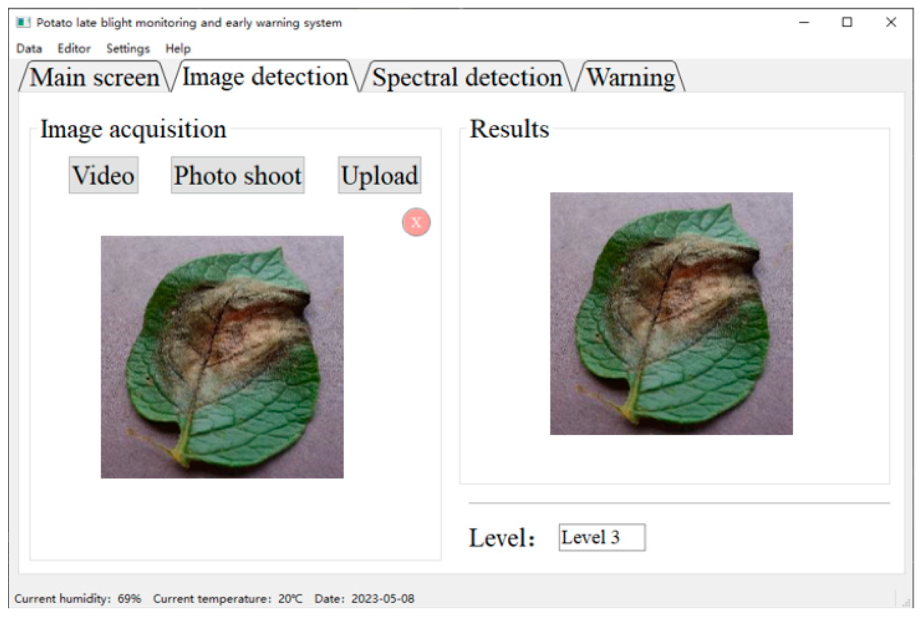
3.5. Embedded Device Deployment

In this study, the control board used was the Raspberry Pi 4B+. The Raspberry Pi is a Linux-based microcomputer motherboard equipped with a 4-core Cortex-A chip, based on ARM architecture. It operates at a main frequency of 1.5 GHz and supports a maximum memory capacity of 8 GB. Under laboratory conditions, a total of 100 potato leaf samples were tested. These samples included 20 healthy leaves, 20 initially diseased leaves, 20 mildly diseased leaves, 20 moderately diseased leaves, and 20 severely diseased leaves. The software’s running interface is shown in Figure 10.

In this study, the precision rate was utilized to assess the effectiveness of disease degree discrimination, and the test results are presented in

Table 11. The results of image-based tests for the detection of late blight.

Category	Number	Precision (%)
Healthy	40	100.0
Late blight Level 1	20	85.0
Late blight Level 2	20	90.0
Late blight Level 3	20	95.0

. The detailed test results can be found in Appendix A. Analyzing Table 11 reveals that the classification precision for healthy leaf images was the highest, followed by late blight 3 leaves, while the recognition of late blight level 1 leaves exhibited the lowest precision. The overall classification precision achieved was 94%. The lower precision in classifying late blight level 1 leaves can be attributed to the fact that, in the early stages of late blight disease, the spots are small and can be easily mistaken for early blight spots. Consequently, late blight level 1 leaves are often misclassified as healthy or early blight level 1 leaves, resulting in poorer classification performance for late blight level 1.

Additionally, this study evaluated the time taken to complete image detection, with the longest detection time as 3.03 s, the shortest time as 3.39 s, and an average time of 3.27 s across the detection of 100 images. The improved model demonstrates better detection speed on embedded devices, meeting the requirements for efficient detection.

4. Conclusions and Prospect

4.1. Conclusions

In this study, we created potato leaf disease datasets, comprising both single and complex contexts. These datasets encompassed seven distinct classes of potato leaf images. To address the class imbalance issue, we applied data augmentation techniques. Subsequently, we achieved fine-grained discrimination of potato leaf diseases using improved lightweight classification networks. The main conclusions of our study are as follows:

(1)

The MobileNet, ShuffleNet, GhostNet, and SqueezeNet pre-trained models, based on the ImageNet dataset, were migrated to the fine-grained classification task using migration training and evaluated comprehensively based on several metrics, including classification accuracy and model complexity. In comparison, the 0.75 MobileNetV3l model has the lowest number of parameters, the ShuffleNetV2 2× model has the fastest inference speed on GPU and CPU, and the GhostNet model has the highest accuracy. Finally, the ShuffleNetV2 2× model, which offers faster CPU inference speed, is chosen as the basic model while ensuring classification accuracy.

(2)

The ShuffleNetV2 2× model was improved by introducing the attention mechanism and adjusting the network structure, and the improvement strategies were: introducing the attention mechanism module, reducing the network depth, and decreasing the number of 1 × 1 convolutions. Compared with the base model, the number of parameters and computational effort of the improved model are substantially reduced, while the classification accuracy increases by 0.85%, and the inference speed on the CPU increases from 25.7 frames per second to 30.2 frames per second. The improved model better balances infer time and accuracy under the premise of reducing model complexity.

(3)

The improved model was deployed and tested in an embedded device, and the overall classification precision was 94%, the average time required for single image detection was 3.27 s, and it had high recognition precision and fast detection speed, which provided important technical support to realize automatic identification of potato late blight diseases.

4.2. Prospect

The software and hardware of the potato late blight detector developed in this research are stable and reliable, and the detection accuracy is high, which has practical application value. In future work, further research can be carried out and improved from the following aspects:

(1)

Enhanced Dataset: Recognizing the importance of data quality and diversity, we will emphasize the need for expanding the potato late blight dataset. This can include gathering more labeled images from different regions, capturing variations in lighting conditions, and incorporating images with different stages and severities of late blight infection.

(2)

Multi-Disease Detection: Given the overlap of symptoms in various plant diseases, we will discuss the possibility of extending the developed deep learning model to detect other plant diseases or multiple diseases simultaneously. This expansion would provide a comprehensive solution for agricultural disease management.

References

1. Sun, D.X.; Shi, M.F.; Wang, Y.; Chen, X.P.; Liu, Y.H.; Zhang, J.L.; Qin, S.H. Effects of partial substitution of chemical fertilizers with organic fertilizers on potato agronomic traits, yield and quality. J. Gansu Agric. Univ. 2023. [Google Scholar] [CrossRef]
2. Liu, P.; Chai, S.; Chang, L.; Zhang, F.; Sun, W.; Zhang, H.; Liu, X.; Li, H. Effects of Straw Strip Covering on Yield and Water Use Efficiency of Potato cultivars with Different Maturities in Rain-Fed Area of Northwest China. Agriculture 2023, 13, 402. [Google Scholar] [CrossRef]
3. Zheng, Z.; Hu, Y.; Guo, T.; Qiao, Y.; He, Y.; Zhang, Y.; Huang, Y. AGHRNet: An attention ghost-HRNet for confirmation of catch-and-shake locations in jujube fruits vibration harvesting. Comput. Electron. Agric. 2023, 210, 107921. [Google Scholar] [CrossRef]
4. Zhao, M.; Jha, A.; Liu, Q.; Millis, B.A.; Huo, Y. Faster Mean-shift: GPU-accelerated Embedding-clustering for Cell Segmentation and Tracking. Med. Image Anal. 2021, 71, 102048. [Google Scholar] [CrossRef] [PubMed]
5. Zhao, M.; Liu, Q.; Jha, A.; Deng, R.; Yao, T.; Mahadevan-Jansen, A.; Tyska, M.J.; Millis, B.A.; Huo, Y. VoxelEmbed: 3D Instance Segmentation and Tracking with Voxel Embedding based Deep Learning. In Proceedings of the International Workshop on Machine Learning in Medical Imaging, Virtual, 17–19 September 2021. [Google Scholar]
6. You, L.; Jiang, H.; Hu, J.; Chang, C.; Chen, L.; Cui, X.; Zhao, M. GPU-accelerated Faster Mean Shift with euclidean distance metrics. In Proceedings of the 2022 IEEE 46th Annual Computers, Software, and Applications Conference (COMPSAC), Virtual, 27 June–1 July 2022. [Google Scholar]
7. Zheng, Z.; Hu, Y.; Yang, H.; Qiao, Y.; He, Y.; Zhang, Y.; Huang, Y. AFFU-Net: Attention feature fusion U-Net with hybrid loss for winter jujube crack detection. Comput. Electron. Agric. 2022, 198, 107049. [Google Scholar] [CrossRef]
8. Gulzar, Y. Fruit Image Classification Model Based on MobileNetV2 with Deep Transfer Learning Technique. Sustainability 2023, 15, 1906. [Google Scholar] [CrossRef]
9. Mamat, N.; Othman, M.F.; Abdulghafor, R.; Alwan, A.A.; Gulzar, Y. Enhancing Image Annotation Technique of Fruit Classification Using a Deep Learning Approach. Sustainability 2023, 15, 901. [Google Scholar] [CrossRef]
10. Gulzar, Y.; Hamid, Y.; Soomro, A.B.; Alwan, A.A.; Journaux, L. A Convolution Neural Network-Based Seed Classification System. Symmetry 2020, 12, 2018. [Google Scholar] [CrossRef]
11. Aggarwal, S.; Gupta, S.; Gupta, D.; Gulzar, Y.; Juneja, S.; Alwan, A.A.; Nauman, A. An Artificial Intelligence-Based Stacked Ensemble Approach for Prediction of Protein Subcellular Localization in Confocal Microscopy Images. Sustainability 2023, 15, 1695. [Google Scholar] [CrossRef]
12. Mohanty, S.P.; Hughes, D.P.; Salathé, M. Using deep learning for image-based plant disease detection. Front. Plant Sci. 2016, 7, 1419. [Google Scholar] [CrossRef] [PubMed] [Green Version]
13. Huang, S.; Sun, C.; Qi, L.; Ma, X.; Wang, W. A deep convolutional neural network-based method for detecting rice spike blight. Trans. Chin. Soc. Agric. Eng. 2017, 169–176. [Google Scholar] [CrossRef]
14. Rahman, C.R.; Arko, P.S.; Ali, M.E.; Khan, M.A.I.; Apon, S.H.; Nowrin, F.; Wasif, A. Identification and recognition of rice diseases and pests using convolutional neural networks. Biosyst. Eng. 2020, 194, 112–120. [Google Scholar] [CrossRef] [Green Version]
15. Barman, U.; Sahu, D.; Barman, G.G.; Das, J. Comparative assessment of deep learning to detect the leaf diseases of potato based on data augmentation. In Proceedings of the 2020 International Conference on Computational Performance Evaluation (ComPE), Shillong, India, 2–4 July 2020. [Google Scholar]
16. Chen, J.; Zhang, D.; Nanehkaran, Y.A.; Li, D. Detection of rice plant diseases based on deep transfer learning. J. Sci. Food Agric. 2020, 100, 3246–3256. [Google Scholar] [CrossRef]
17. Suarez Baron, M.J.; Gomez, A.L.; Diaz, J.E.E. Supervised Learning-Based Image Classification for the Detection of Late Blight in Potato Crops. Appl. Sci. 2022, 12, 9371. [Google Scholar] [CrossRef]
18. Eser, S. A deep learning based approach for the detection of diseases in pepper and potato leaves. Anadolu Tarım Bilim. Derg. 2021, 36, 167–178. [Google Scholar]
19. Hughes, D.; Salathé, M. An open access repository of images on plant health to enable the development of mobile disease diagnostics. arXiv 2015, arXiv:1511.08060. [Google Scholar]
20. GB/T 17980.34-2000; Pesticides Field Efficacy Test Guidelines (I) Fungicide Control of Potato Late Blight. The Ministry of Agriculture and Rural Affairs of the People’s Republic of China: Beijing, China, 2000.
21. Mikołajczyk, A.; Grochowski, M. Data augmentation for improving deep learning in image classification problem. In Proceedings of the 2018 International Interdisciplinary PhD Workshop (IIPhDW), Świnouście, Poland, 9–12 May 2018. [Google Scholar]
22. Ma, N.; Zhang, X.; Zheng, H.-T.; Sun, J. Shufflenet v2: Practical guidelines for efficient cnn architecture design. In Proceedings of the European Conference on Computer Vision (ECCV), Munich, Germany, 8–14 September 2018. [Google Scholar]
23. Hu, J.; Shen, L.; Sun, G. Squeeze-and-excitation networks. In Proceedings of the IEEE Conference on Computer Vision and Pattern Recognition, Salt Lake City, UT, USA, 18–23 June 2018. [Google Scholar]
24. Woo, S.; Park, J.; Lee, J.-Y.; Kweon, I.S. Cbam: Convolutional block attention module. In Proceedings of the European Conference on Computer Vision (ECCV), Munich, Germany, 8–14 September 2018. [Google Scholar]
25. Wang, Q.; Wu, B.; Zhu, P.; Li, P.; Zuo, W.; Hu, Q. ECA-Net: Efficient channel attention for deep convolutional neural networks. In Proceedings of the IEEE/CVF Conference on Computer Vision and Pattern Recognition, Seattle, WA, USA, 13–19 June 2020. [Google Scholar]
26. Li, H.; Qiu, W.; Zhang, L. Improved ShuffleNet V2 for Lightweight Crop Disease Identification. Comput. Eng. Appl. 2022, 58, 260–268. [Google Scholar]
27. Zhang, X.; Zhou, X.; Lin, M.; Sun, J. Shufflenet: An extremely efficient convolutional neural network for mobile devices. In Proceedings of the IEEE Conference on Computer Vision and Pattern Recognition, Salt Lake City, UT, USA, 18–23 June 2018. [Google Scholar]
28. Howard, A.G.; Zhu, M.; Chen, B.; Kalenichenko, D.; Wang, W.; Weyand, T.; Andreetto, M.; Adam, H. Mobilenets: Efficient convolutional neural networks for mobile vision applications. arXiv 2017, arXiv:1704.04861. [Google Scholar]
29. Sandler, M.; Howard, A.; Zhu, M.; Zhmoginov, A.; Chen, L.-C. Mobilenetv2: Inverted residuals and linear bottlenecks. In Proceedings of the IEEE Conference on Computer Vision and Pattern Recognition, Salt Lake City, UT, USA, 18–23 June 2018. [Google Scholar]
30. Howard, A.; Sandler, M.; Chu, G.; Chen, L.-C.; Chen, B.; Tan, M.; Wang, W.; Zhu, Y.; Pang, R.; Vasudevan, V. Searching for mobilenetv3. In Proceedings of the IEEE/CVF International Conference on Computer Vision, Seoul, Republic of Korea, 27 February 2020. [Google Scholar]
31. Han, K.; Wang, Y.; Tian, Q.; Guo, J.; Xu, C.; Xu, C. Ghostnet: More features from cheap operations. In Proceedings of the IEEE/CVF Conference on Computer Vision and Pattern Recognition, Seattle, WA, USA, 13–19 June 2020. [Google Scholar]
32. Iandola, F.N.; Han, S.; Moskewicz, M.W.; Ashraf, K.; Dally, W.J.; Keutzer, K. SqueezeNet: AlexNet-level accuracy with 50x fewer parameters and< 0.5 MB model size. arXiv 2016, arXiv:1602.07360. [Google Scholar]
33. Hong, H.; Lin, J.; Huang, F. Tomato disease detection and classification by deep learning. In Proceedings of the International Conference on Big Data, Artificial Intelligence and Internet of Things Engineering (ICBAIE), Fuzhou, China, 12–14 June 2020; IEEE: New York, NY, USA, 2020; pp. 25–29. [Google Scholar]
34. Osama, R.; Ashraf, N.E.H.; Yasser, A.; AbdelFatah, S.; El Masry, N.; AbdelRaouf, A. Detecting plant’s diseases in Greenhouse using Deep Learning. In Proceedings of the 2020 2nd Novel Intelligent and Leading Emerging Sciences Conference (NILES), Giza, Egypt, 24–26 October 2020; IEEE: New York, NY, USA, 2020; pp. 75–80. [Google Scholar]
35. Rozaqi, A.J.; Sunyoto, A. Identification of disease in potato leaves using Convolutional Neural Network (CNN) algorithm. In Proceedings of the 2020 3rd International Conference on Information and Communications Technology (ICOIACT), Yogyakarta, Indonesia, 24–25 November 2020; IEEE: New York, NY, USA, 2020; pp. 72–76. [Google Scholar]
Figure 1. Examples of PLDD images. (a) Early stages of late blight leaf in a single context. (b) End stages of late blight leaf in a single context. (c) Early stages of early blight leaf in a single context. (d) End stages of early blight leaf in a single context. (e) Healthy leaf in a single context. (f) Early stages of late blight leaf in a natural context. (g) End stages of late blight leaf in a natural context. (h) Early stages of early blight leaf in a natural context. (i) End stages of early blight leaf in a natural context. (j) Healthy leaf in a natural context.
Agronomy 13 01659 g001
Figure 2. Examples of PLDD images after leaf annotation. (a) Original image of late blight leaf. (b) late blight leaf after annotation.
Agronomy 13 01659 g002
Figure 3. The process of extraction of diseased areas.
Agronomy 13 01659 g003
Figure 4. The structure of ShuffleNetV2 units. (a) The structure of Stride = 1 unit; (b) The structure of Stride = 2 unit.
Agronomy 13 01659 g004
Figure 5. The structure of the ECA module.
Agronomy 13 01659 g005
Figure 6. Different forms of Shuffle-Attention module structure. (a) The structure of Shuffle-Attention-A; (b) The structure of Shuffle-Attention-B; (c) The structure of Shuffle-Attention-C.
Agronomy 13 01659 g006
Figure 7. The accuracy curve of the training set and the validation set. (a) training set; (b) validation set.
Agronomy 13 01659 g007
Figure 8. The structure of ShuffleNetV2 2×—improved model. Note: Stage 2, Stage 3 and Stage 4 are all composed of the original base unit, with Stride = 1, and the modified unit is composed of Stride = 1 unit and Stride = 2 unit. (1, 1, 2, 1) in Stage2 indicates one stack of unit (a) with improved Stride = 2, one stack of unit (b) with improved Stride = 1, two stacks of basic unit with original Stride = 1, and one stack of unit (c) with improved Stride = 1; (1, 1, 5, 1) in Stage3 indicates one stack of unit (a) with improved Stride = 2, one stack of unit (b) with improved Stride = 1, five stacks of basic unit with original Stride = 1, and one stack of unit (c) with improved Stride = 1; (1, 1, 1, 1) in Stage4 indicates one stack of unit (a) with improved Stride = 2, one stack of unit (b) with improved Stride = 1, one stack of basic unit with original Stride = 1, and one stack of unit (c) with improved Stride = 1.
Agronomy 13 01659 g008
Figure 9. The confusion matrix for fine-grained classification results of PLDD images.
Agronomy 13 01659 g009
Figure 10. Image detection operation interface.
Agronomy 13 01659 g010