1. Introduction
Precision agriculture, which is aimed at reducing the cost of agricultural production, environmental pollution and the automation of crop management [
1], is gaining widespread attention and is being investigated by various agricultural researchers. In precision agriculture, the accurate acquisition of crop status and position is crucial for facilitating precise fertilization, weed control and full automation of crop management [
2]. It serves as a key factor in reducing fertilizer waste, excessive herbicide use and controlling costs [
3,
4]. Crop detection becomes more challenging during the seedling stage, as crop seedlings bear a resemblance to weeds and are more susceptible to death from possible environmental factors. Hence, the design of a model capable of accurately detecting crop seedlings in complex environments becomes increasingly crucial.
In the past, crop detection often focused on individual crop species as targets and utilized conventional visual algorithms for detection [
5,
6]. Gai et al. [
7] used the 2D connected components method, two-dimensional multiscale wavelet transformation and marker-controlled watershed segmentation algorithm to segment broccoli and lettuce. The accuracy for segmenting broccoli and lettuce achieved 92.4% and 96.6%, respectively. Chen et al. [
8] extracted Gabor features from corn images and built a support vector machine (SVM) model to learn the Gabor features of corn images for corn detection. In addition, Hamuda et al. [
9] used cauliflower HSV spatial images as input for cauliflower detection based on the dilation algorithm and moment method, which obtained a detection accuracy of 99.04%.
With the development of deep learning, convolutional neural networks (CNN) were developed, a vision algorithm with a stronger generalization ability and higher accuracy compared to traditional vision algorithms. CNN neural networks are widely used in precision agriculture and smart agriculture, such as automatic species identification [
10], disease identification [
11,
12] and fruit ripeness analysis [
13,
14,
15]. Most of the research on crop and weed localization is based on object detection networks, such as You Only Look Once (YOLO) [
16,
17,
18,
19] series models and Region-CNN (RCNN) series models [
20,
21,
22]. Zou et al. [
23] combined images with and without weeds to generate new weed images, and trained a semantic segmentation network called UNet, obtaining an accuracy of 92.21%. Punithavathi et al. [
24] proposed a detection model based on Faster RCNN for crop and weed detection and used the extreme learning machine algorithm to optimize the hyperparameters of the deep learning model to obtain a higher detection accuracy. Chen et al. [
25] detected weeds in sesame fields based on the YOLOv4 detection network and used local attention pooling to replace maximum pooling in spatial pyramid pooling and SEnet modules to replace logical modules in local attention pooling. The model obtained a 96.16% detection accuracy. Although these studies have provided a solid theoretical and experimental foundation for crop detection, the development of comprehensive automated crop management is still challenging. One of these challenges is that current studies mainly focus on crops that have grown to a degree where they can be easily distinguished from their surroundings. Another challenge is the precise localization of crops with dense planting (placing multiple seeds in a single planting hole), particularly during the seedling stage.
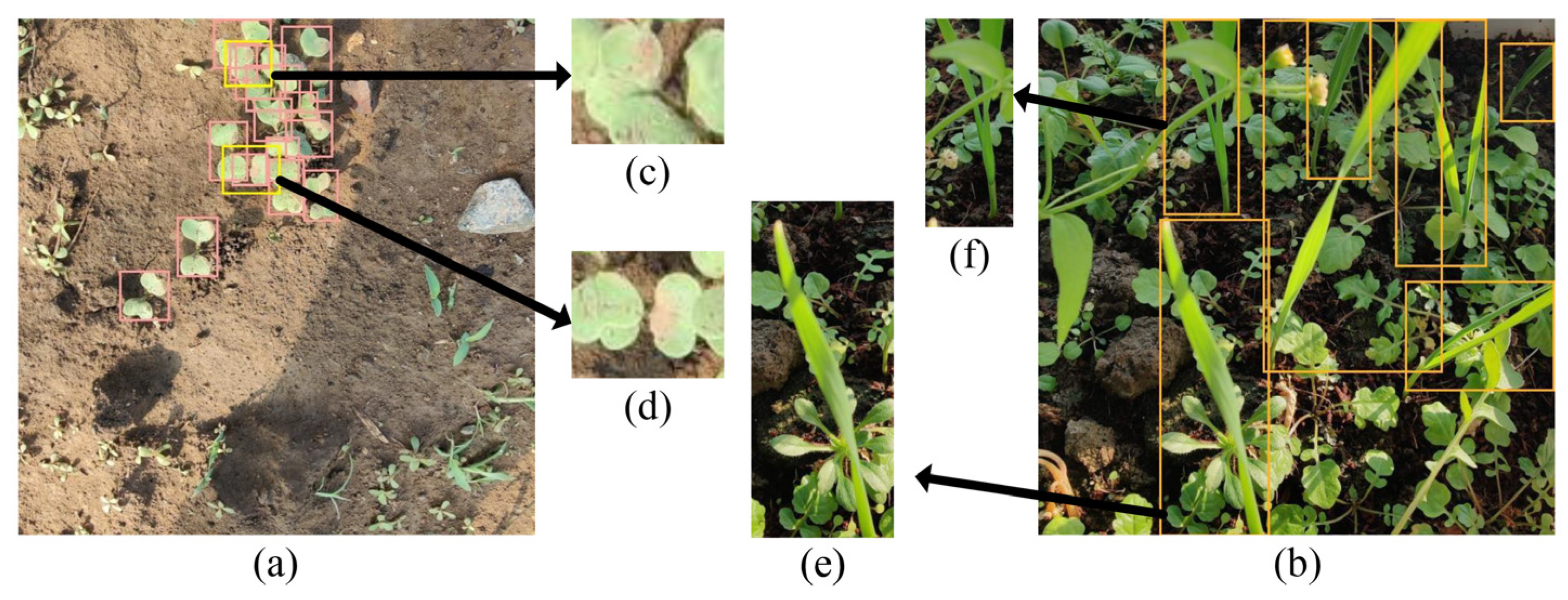
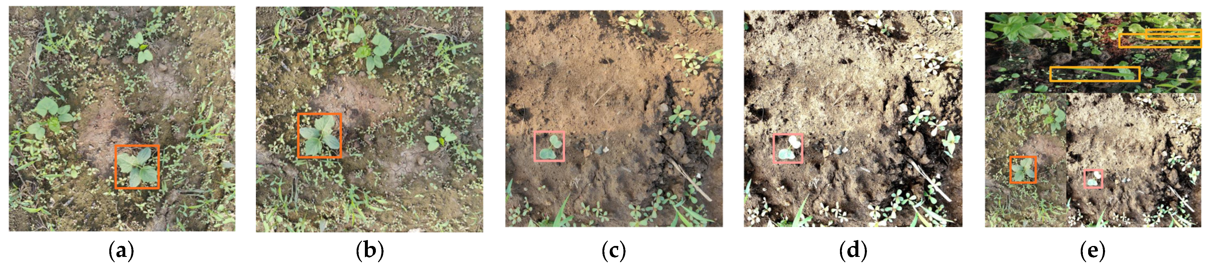
Additionally, we have identified several issues regarding the labeling process. In previous detection studies, researchers typically labeled the entire crop as the target, as shown in
Figure 1a,b. However, this method presented three potential issues.
The first issue was that because of the dense nature of the crops, as shown in
Figure 1d, the worker needs to be meticulous to identify multiple leaves belonging to the same crop. This process will produce errors in labeling. The second issue was that some crops can only be labeled to a single leaf due to occlusion, as shown in
Figure 1c. As a result, there was a significant gap in the information about the same target features, making it difficult for the deep learning model to learn the feature patterns and reducing identification accuracy. Lastly, the third issue is that crops exhibit different growth rates, resulting in some crops having only one leaf, while others may have multiple leaves, as shown in
Figure 1e,f. This inconsistency also reduced the detection accuracy. Although the whole crop labeling method can aid in identifying each crop, these three scenarios can lead to labeling errors. Additionally, in some cases, there may be a significant difference in the shape of the target, which can result in reduced accuracy for detecting the crop. Therefore, it is important to develop more effective labeling strategies to improve the accuracy of crop detection.
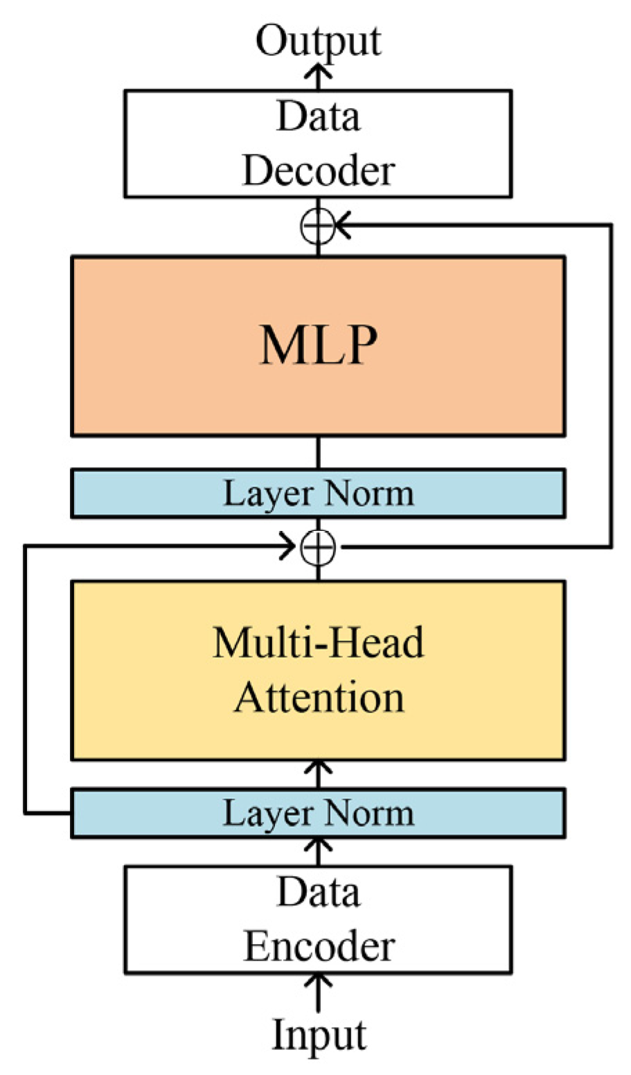
To address the issue of low accuracy in detecting crops from dense crop seedlings in complex environments, we constructed a crop seedling dataset that included crops such as soybean, wheat, radish and cucumber, grown with different planting methods, sizes and growing environments. In addition, two labeling strategies were proposed in a scientific manner for dense planting crops. Furthermore, we proposed a deep learning structure transformer mechanism applied to computer vision that has been investigated recently. Since the transformer mechanism has been shown to be more resistant to interference and to extract features more rationally [
26,
27], it improves both the detection and recognition accuracy when combined with convolutional neural networks [
28]. Therefore, we took inspiration from these studies that incorporated the transformer mechanism into their CNN-based model and expected to improve the detection accuracy of the model for various crop seedlings in complex environments.
In summary, we carried out the following work:
An image dataset was constructed, comprising seedlings from four different crops, all grown in environments with a substantial weed presence. Additionally, a dense planting method was used for some crops.
In order to improve the accuracy of the model for the detection of densely grown crops, two labeling strategies were proposed from the perspective of crop type.
A detection model for dense targets based on YOLOv5 and the transformer mechanism was proposed from the perspective of model structure.
Finally, in order to improve the detection efficiency, the model was lightened and improved based on the impact of three different features in the transformer mechanism on the accuracy.
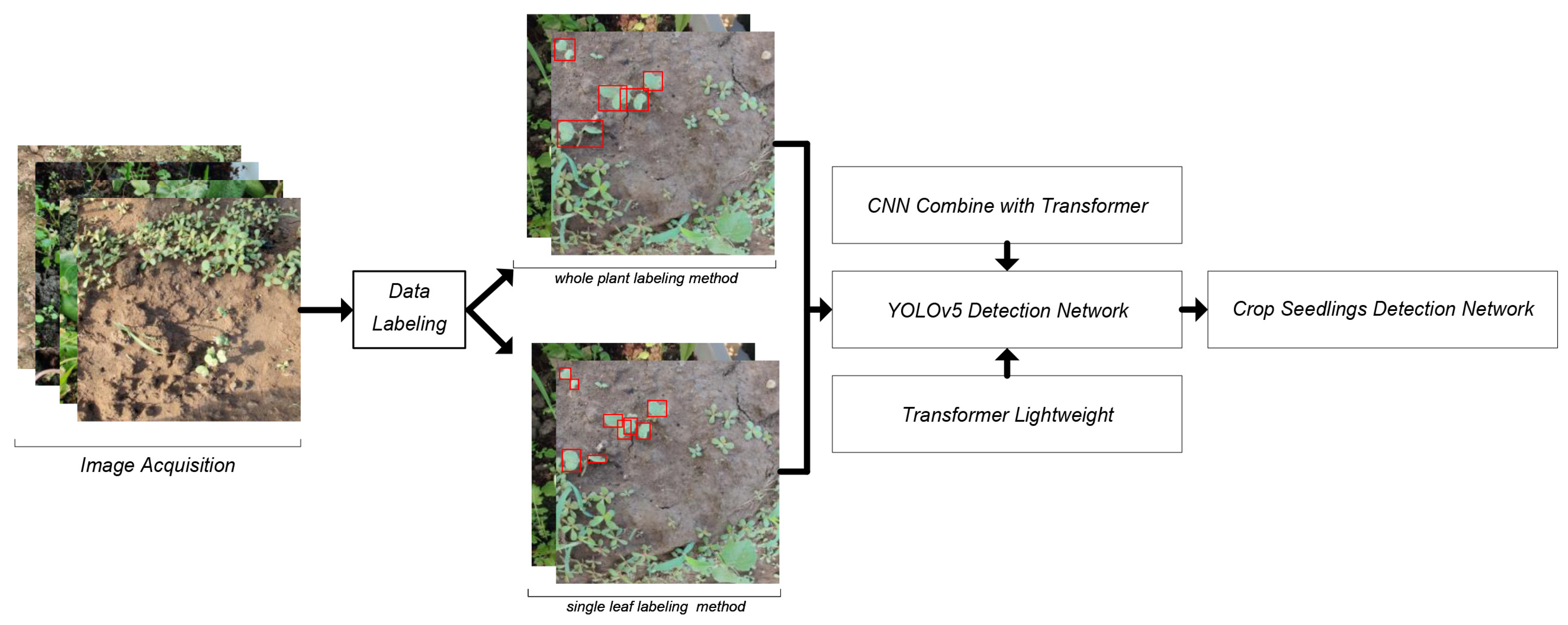
The workflow diagram of the study is shown in
Figure 2.
2. Materials and Methods
2.1. Image Acquisition
The image capture device was a smartphone Oneplus8P (the manufacturer was BBK Electronics, Shenzhen, China), with a main camera lens of 48 million pixels, and the captured picture pixels were 3000 × 3000. The camera’s ISO was set to 400, the color temperature was set to 5000 and the shutter speed was set to 1/50 s. The photographs were taken at a height ranging from 20 to 40 cm. In total, we collected 2140 digital RGB images in JPG format for use in this study.
In order to improve the model’s generalization capacity and validate its efficacy in detecting a wide range of crops in complex environmental conditions, we meticulously built a dataset of crop seedlings with our own shooting. These data would be used to train and validate the model.
Four crops were targeted, namely soybeans, radishes, cucumbers and wheat. These crops were specifically chosen for two reasons. Firstly, soybean, radish, cucumber and wheat are representative cash crops. Secondly, the seedling stages of various weed species, such as setaria viridis, eleusine indica, wild pea and petunia, bear resemblance to the seedling stages of the aforementioned crops.
The cultivation of these crops took place within a greenhouse located at Jilin Agricultural University in China. The greenhouse measures 5 m in width and 40 m in length. To create an environment rich in weed species, no weeding was conducted prior to crop planting and throughout the crop cultivation process. Specifically, soybeans and wheat were directly and randomly sown in the field, while cucumbers were planted at 20 cm intervals with 1–3 seeds placed in each planting hole. Radishes were also planted at 20 cm intervals, with more than 5 radish seeds placed in each planting hole. A total of 50 soybean and wheat seeds were planted, 27 cucumber seeds were planted and 30 planting holes were utilized for radishes.
During the seedling stage of the crops, the entire crop was photographed. Specifically, for soybeans, the seedling stage refers to the period from the emergence of cotyledons to the growth of the third true leaf. The same applies to cucumbers. For radishes, the seedling stage specifically refers to the period from the emergence of cotyledons to the growth of the first true leaf. As for wheat seedlings, the seedling stage refers to the period when the entire crop is less than 15 cm in height. Thirty specimens of each crop were planted and photographs were taken every three days starting from when the first pair of true leaves fully unfolded.
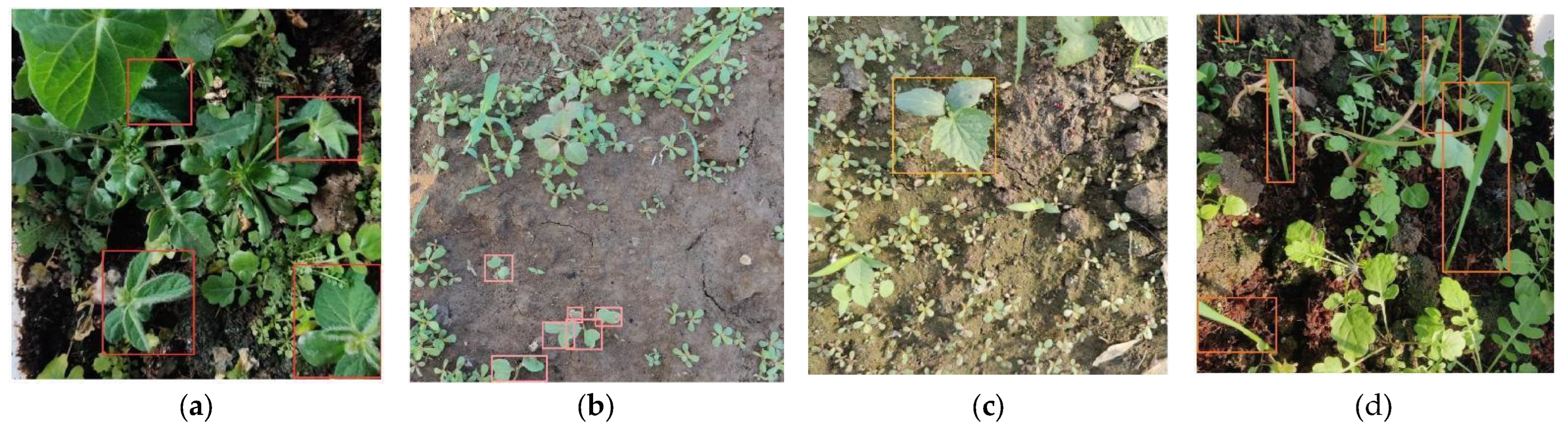
The crop seedling data comprised soybean, which was of medium size and planted sparsely, resulting in partial obscurity by weeds (
Figure 3a), making detection slightly difficult (the size represents the proportion of the target crop in the entire image). Similarly, radish was small and densely planted, with seedlings not obscured by weeds but covered by other radish seedlings (
Figure 3b), making it more challenging to detect. In addition, the cucumber was of medium size, planted sparsely and not shaded by other weeds, resulting in the least difficult detection (
Figure 3c). Although wheat was planted sparsely, the seedlings were still be covered by other seedlings, which was the same for that of densely planted radishes (
Figure 3d), which greatly increased the difficulty of detection. Detailed information on the data of each crop seedling is shown in
Table 1. The dataset was split into training and test sets with the ratio of 0.8:0.2.
2.2. Labeling Strategy and Data Enhancement
To match the model input size and address the GPU memory limitations, we first reduced the image resolution from 3000 × 3000 to 640 × 640 using bilinear interpolation. Then, Labelimg 1.8.1 (an open source, efficient image labeling tool) was used to label the crop images and the tag data format was set to VOC format.
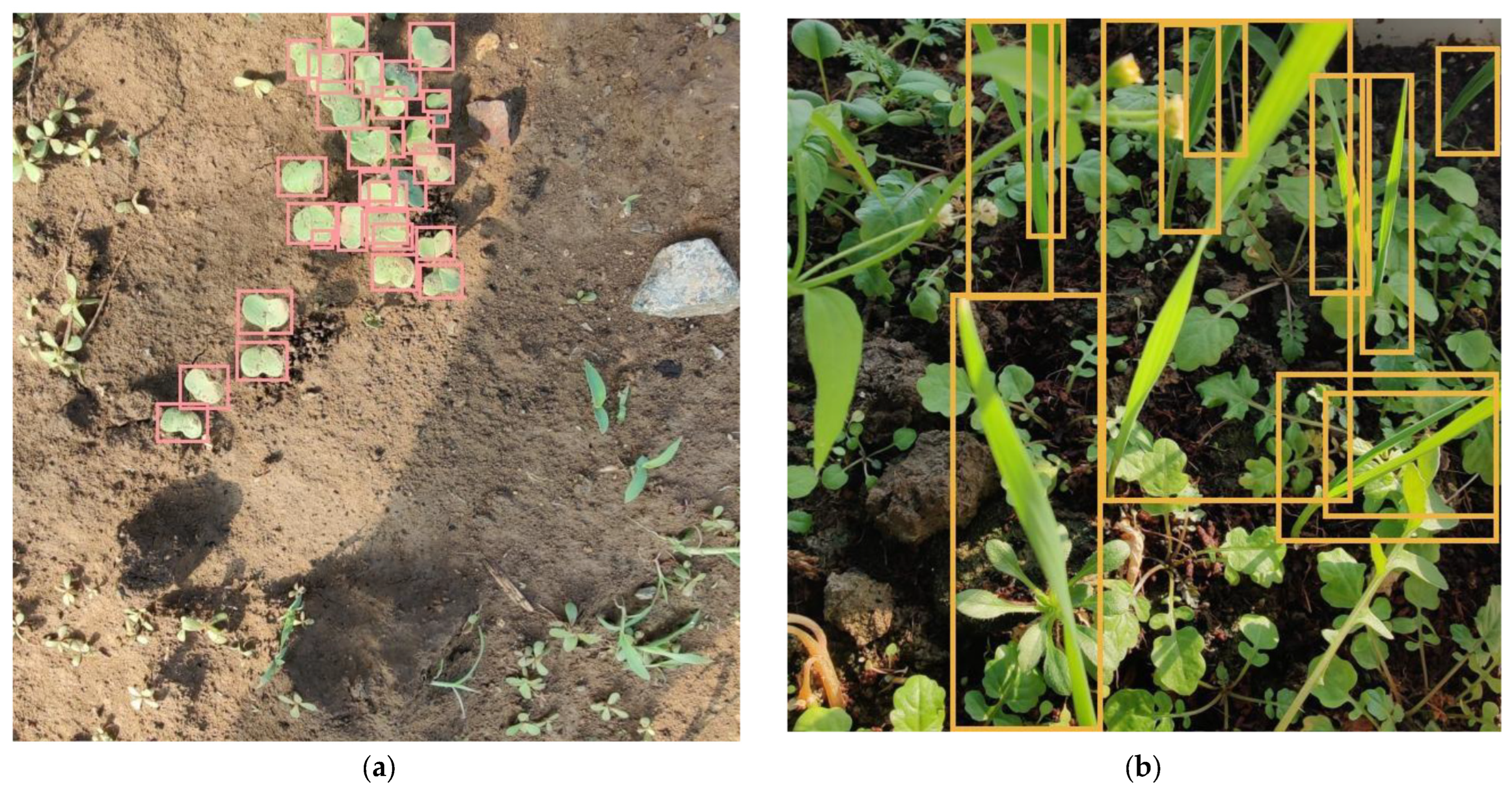
On the basis of the whole crop labeling method, we proposed the second labeling strategy as another possible option, referred to it as Strategy B, which utilized the single leaf labeling method, as shown in
Figure 4. This labeling method has the following advantages. This method involved labeling a single leaf, thereby effectively reducing the labeling difficulty. Workers only needed to label each individual leaf without considering the logical relationship between the leaves. In addition, this method resulted in a more uniform target morphology and clearer features within the labeling box, particularly in cases of dense planting. By adopting this new labeling strategy, the study was able to overcome the limitations of the whole crop labeling method as stated in the introduction and improve the accuracy in crop detection.
To avoid model overfitting and to enhance the model performance, the amount of training data was expanded by employing various techniques. Two popular methods are image enhancement and mosaic enhancement. The image enhancement method involves applying random rotation and color dithering to the images. The color dithering operation adjusts various image properties such as image saturation, sharpness, brightness and contrast. The values of saturation and sharpness range from 0 to 3.1 and the values of luminance and contrast range from 1 to 2.1. The mosaic enhancement method takes a different approach by creating a single image from multiple randomly selected images. This process involved flipping and scaling the images, dithering the colors and finally stitching them together into a single image. The mosaic method allows the model to learn multiple images simultaneously, which improves the generalization ability of the model. A schematic diagram of the above two expansion methods is shown in
Figure 5. The image enhancement was run online by the program, and it did not affect the original data. The enhancement probability we set was 50%, that is, there was a 50% possibility of enhancing the input image in one round of training.
2.3. Crop Seedlings Detection Network
The YOLOv5 is a single-stage target detection model, which is the most mature model in the YOLO series of models [
29]. Compared to YOLOv3 [
30] and YOLOv4 [
31], YOLOv5 achieves a higher computational accuracy and minimal arithmetic power consumption. The model is continuously updated, making it more mature compared to YOLOv7 [
32] and it outperforms its predecessors in various fields [
33,
34]. Therefore, YOLOv5 was used as the base detection network in this study.
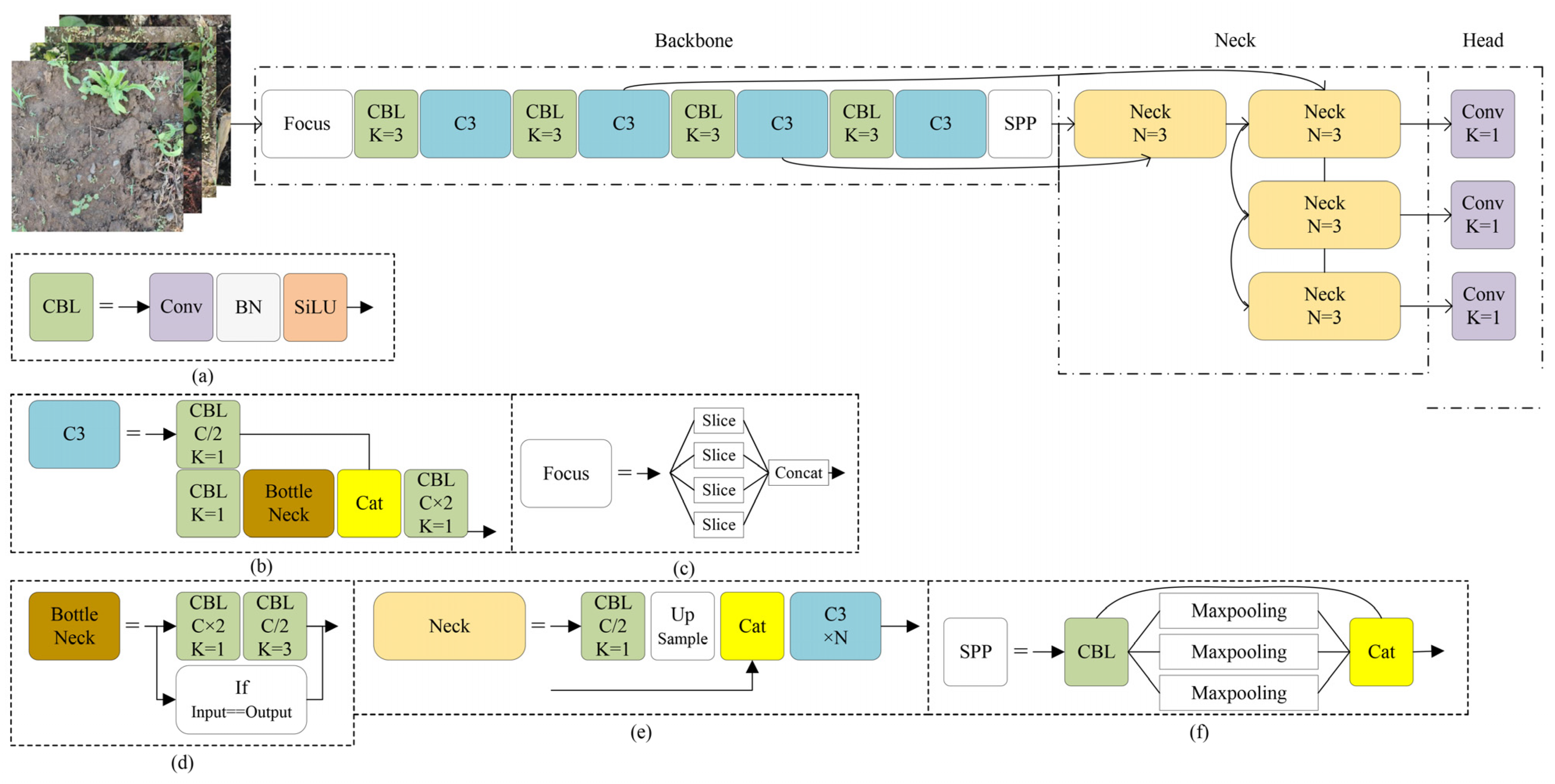
The YOLOv5 structure consists of three main parts. Through these three structures, the model could effectively extract image features and locate key areas. The schematic diagram of the model structure is shown in
Figure 6. The first part employed an improved cross-stage partial network (CSPNet) as the backbone network to extract the image-based feature information [
35]. To improve the feature extraction, the faster feature extraction C3 module and the spatial pyramid pooling (SPP) that unifies multiple scale feature maps into the same size were added to CSPNet [
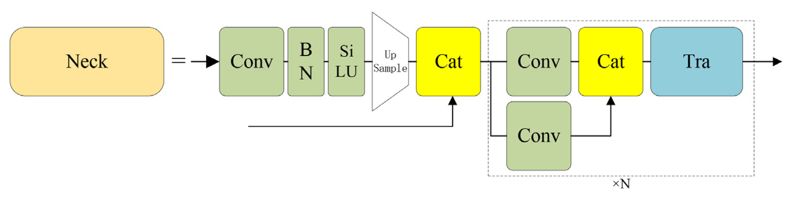
20]. The second part was the neck network that extracted and processed the base image feature information output from the backbone network. To accomplish this, it used the feature pyramid network (FPN) structure [
36], which consists of several neck blocks that perform computation and feature fusion. The neck blocks were responsible for aggregating the feature map information in the previous layer of neck blocks or the backbone network. The third component of the model was the detection head. Its primary purpose is for calculating relevant information of the detected targets in the detection box, such as the confidence level and the length and width adjustment value of the detection box. The detection head comprises three sub-components, each with a different feature map size, 76 × 76, 38 × 38, and 19 × 19, respectively. These sub-components detect small-sized, medium-sized and large-sized objects, respectively.
2.4. Training Settings and Hyperparameters
The optimization function used to train the model in this paper was the SGD function. The classification loss used the focal loss function to address the issue of imbalanced data caused by the higher number of crops in the densely grown crop images compared to the sparsely grown crops [
42]. The detection loss was calculated using the IOU function [
43], and the NMS (Non-Maximum Suppression) method [
44] was used to filter redundant detection boxes. To effectively accelerate the model learning speed, we applied the OneCycleLR method for the learning rate. To obtain the optimal detection results of the model on the crop seedling dataset of this paper, we fine-tuned the hyperparameters of YOLOv5, as shown in
Table 2. Among them, depth and width, which control the depth and width of the model, were kept constant. To obtain the optimal hyperparameters, the model underwent 500 training iterations, each consisting of 30 epochs. After each training iteration, we adjusted the hyperparameters and finally obtained the optimal set of hyperparameters with the highest accuracy during testing.
2.5. Experimental Equipment
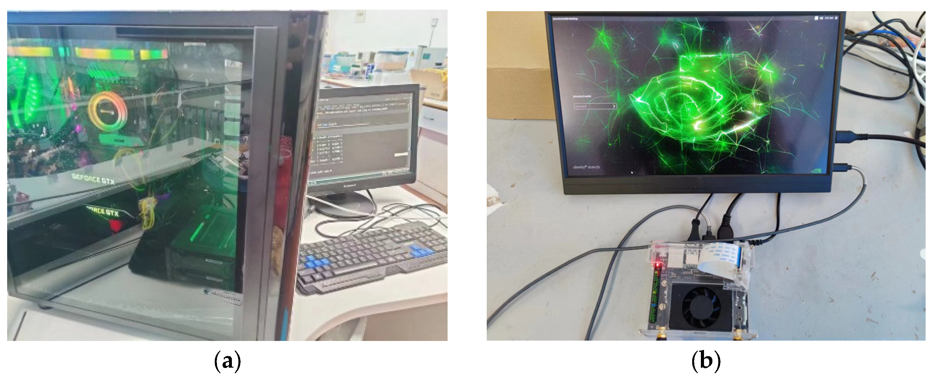
The experiments were conducted on a Windows 10 operating system, using an NVIDIA Titan X GPU and Intel Xeon E5-2696 v3 CPU to train the deep learning models in PyTorch 1.7.0 with Python 3.6. The experimental device utilized for training the model is shown in
Figure 9a.
The Jetson TX2 (as shown in
Figure 9b) operating system was Ubuntu 18.04 using the deep learning framework Pytorch 1.8. The CPU was a CPU cluster consisting of a dual-core Denver2 processor and a quad-core ARM Cortex-A57, with 4 GB of LDDR4 memory and a 256-core Pascal GPU.
2.6. Performance Evaluation
To measure the performance of each trained model on the testing set, evaluation indicators were used in this study. Specifically, we evaluated the model performance by single species average precision (AP), mean detection precision (mAP), floating-point operations per second (FLOPs), computational speed of the training platform (server speed) and the computational speed of the carrying platform (TX2 speed). The unit of speed was ms·frame
−1, which was how long it took to calculate a frame. The AP was determined by precision and recall, the formula of precision is shown in Equation (4) and the formula of recall is shown in Equation (5), where
TP is true positive,
FP is false positive and
FN is false negative.
TP,
FP and
FN are determined by the IOU threshold. The IOU value is the overlap area between the detection box calculated by the model and the manually labeled detection box.
The formula for calculating AP is shown in Equation (6) and the value of the IOU was taken as 0.5 when evaluating the AP for a single crop. The mAP is the mean value of AP for the four species. The mAP had different IOU values. The mAP was named mAP0.5 when the value of the IOU was 0.5. The mAP0.5–0.95 was the mean value of the AP for the four species between IOU thresholds from 0.5 to 0.95 at intervals of 0.05 to calculate the AP. This index represented a more rigorous evaluation of the detection accuracy.
Floating-point operations (FLOPs) measure the computational memory consumed by the model for each operation in the convolutional and fully connected layers during forward propagation of the model. The formula for calculating the FLOPs is displayed in Equation (7), where
Ci is the convolutional layer input channel and
K is the convolution kernel size.
H and
W are the height and weight of the convolutional layer output feature map, respectively, and
Co is the output channel.
I and O are the input and output numbers in the fully connected layers, respectively. The unit of
FLOPs is
G (Giga)
3. Results
3.1. Results of Two Strategies and Transformer
The results obtained from the models on the testing set are shown in
Table 3. In strategy A, the AP of the model with the transformer was improved for soybean (results of YOLOv5, YOLOv5ViT and YOLOv5ST: 90.0–91.4–91.9%), radish (77.3–80.7–81.1%) and cucumber (91.9–94.3–95.3%), demonstrating that the transformer mechanism could enhance the accuracy of the model for both dense and sparse sowing densities. However, we found that the AP for wheat was not significantly improved or even reduced. This is because wheat is planted densely and the wheat leaves are slender in shape, resulting in each detection box containing too many background features. As a result, the model was unable to focus on the region of interest of wheat.
This result also confirms our hypothesis that a large discrepancy in the feature information within the detection boxes of objects of the same category can lead to a reduction in precision. In strategy B, the same high AP was maintained for both sparsely planted cucumbers and soybeans, and an even higher AP was achieved for the model with the transformer mechanism. With strategy B, the detection box size of wheat was reduced, making each detection box contain only one leaf and reducing the feature gap in the detection box of the wheat. However, the characteristic of wheat leaves still caused too many background features to be included in the box, resulting in more dense detection boxes and a lower wheat AP for YOLOv5. Nonetheless, we observed that the model with transformer mechanism significantly improved the detection accuracy of wheat relative to strategy A (results of strategy A: 73.2–73.7–72.9%; results of strategy B: 72.7–74.0–73.1%), indicating that the transformer mechanism is well-suited for detection in complex environments and medium-sized targets.
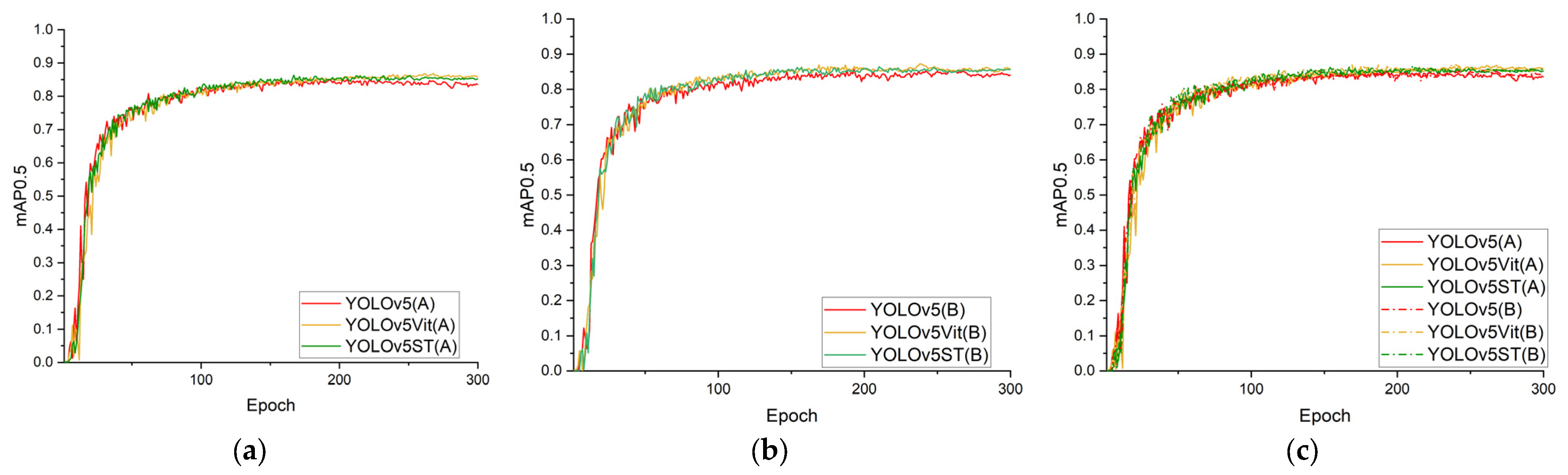
The training accuracy curves for YOLOv5, YOLOv5 ViT and YOLOv5 ST are shown in
Figure 10. The curves showed that all three models achieved convergence after about 100 rounds. Because the underlying networks were based on YOLOv5, the curves displayed similar trends across the three models, as shown in
Figure 10a. The model using strategy A had a large oscillation of the accuracy curve, especially before 100 epochs, as shown in
Figure 10b. The large oscillation represents the difficulty of the model to learn the feature patterns, thereby highlighting the issue of a large gap in the information of the target individual features that existed in the overall labeling method. The model using strategy B, as shown in
Figure 10c, had a lower initial accuracy due to the greater number of targets to be detected in each image. However, the gap in each individual feature’s information was relatively small, the oscillation amplitude was lower and the accuracy improved more rapidly.
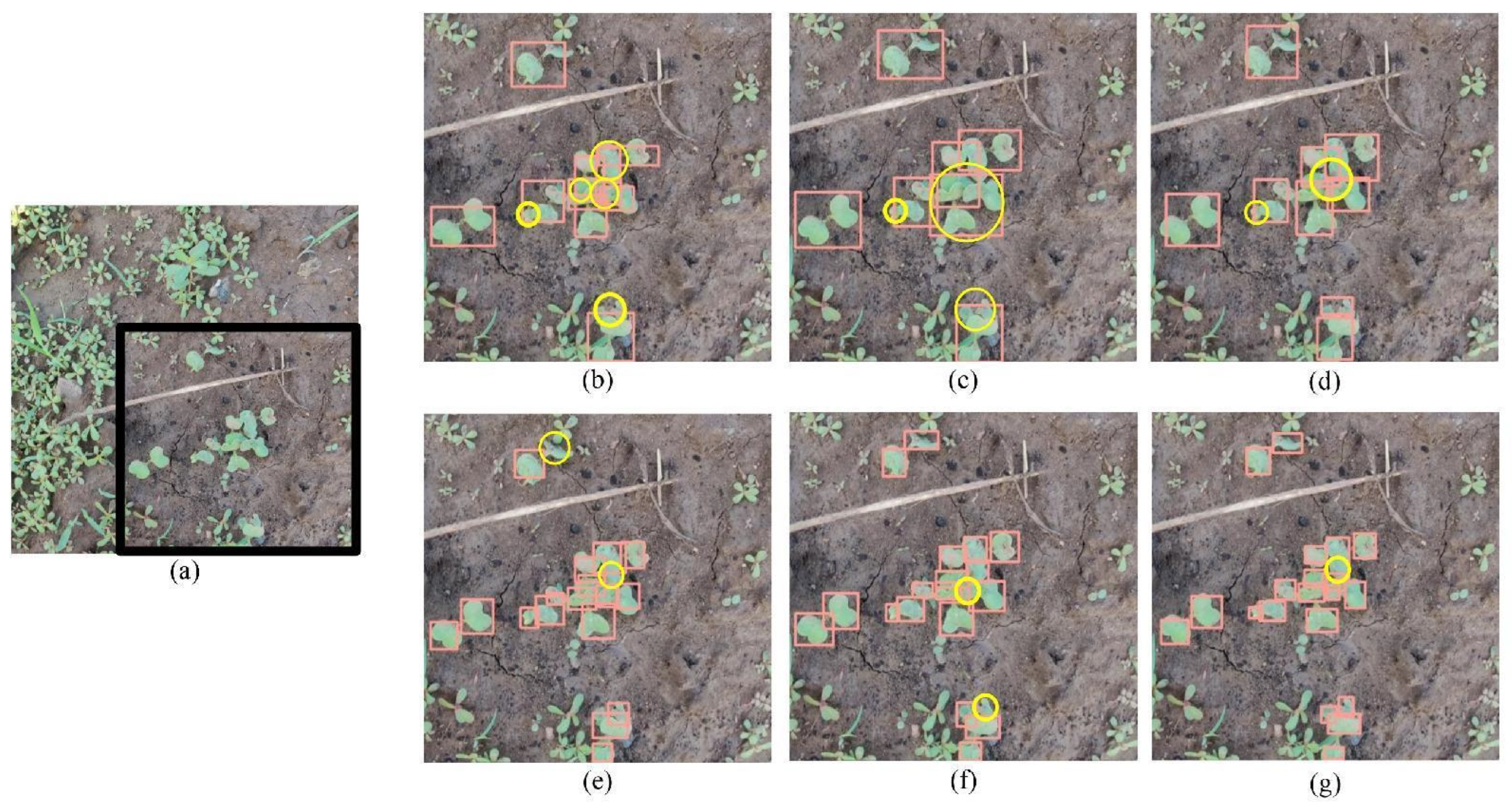
Although the mAP of strategy B did not show a significant improvement compared to strategy A, it has practical advantages in detecting individual crops. As shown in the detection map of radishes in
Figure 11, strategy B provided information on each crop, even if it was only partial, as shown in
Figure 11e–g. In contrast, strategy A produced missed individuals as shown in the detection images b, c and d. Therefore, despite the slight difference in the mAP, strategy B can provide more comprehensive and accurate information on individual crops, resolving the problem of difficult feature learning due to strategy A.
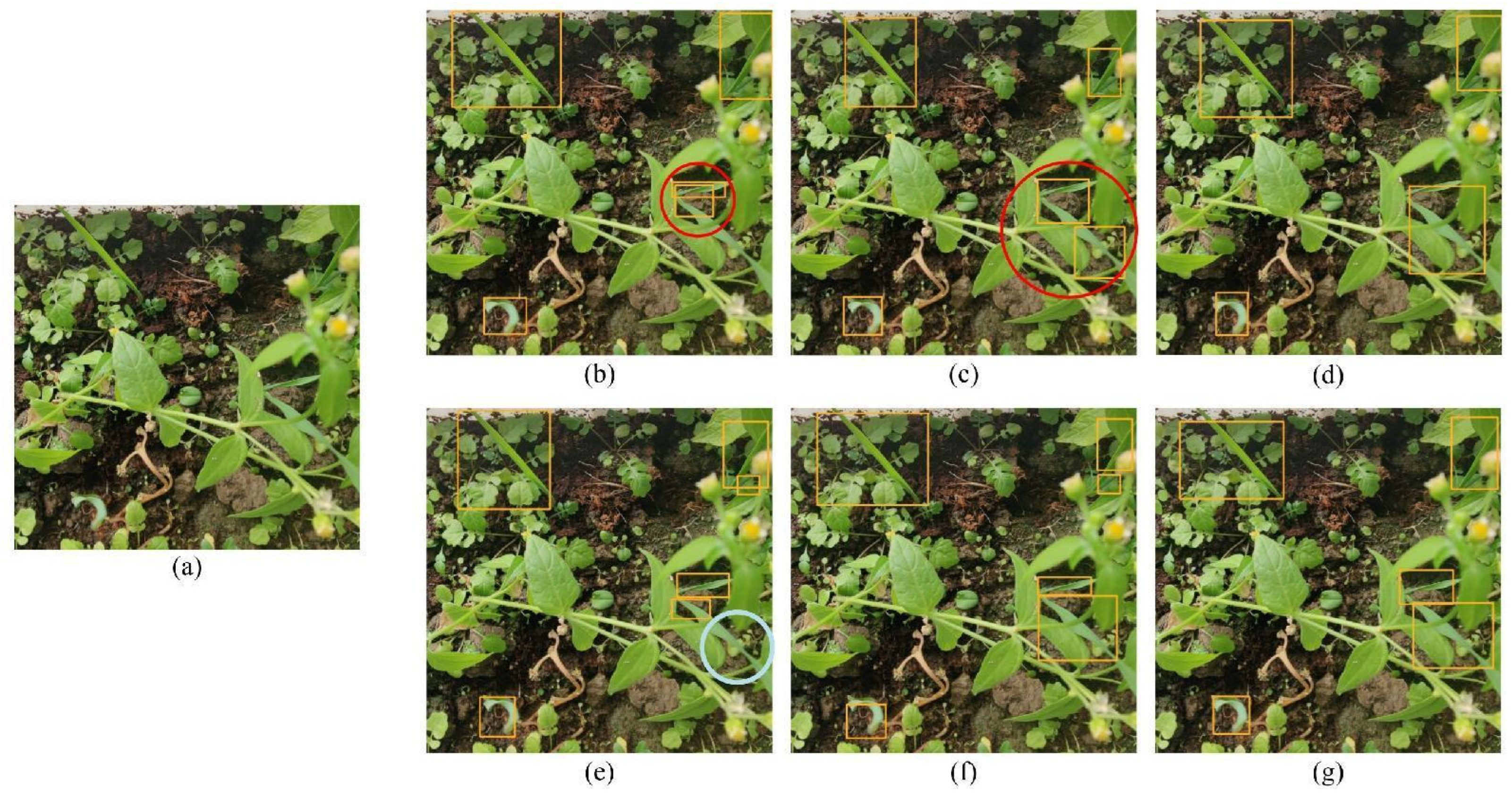
The results of the wheat assay are shown in
Figure 12. Although the whole crop labeling method was used (strategy A), multiple detection boxes for one crop were produced in the red circles (
Figure 12b,c). This phenomenon is more akin to the single leaf labeling method. In addition, the phenomenon observed in
Figure 12b highlighted the potential issue that crops with different numbers of leaves can lead to box selection confusion problems. The results in
Figure 12c highlighted another potential issue of the presence of crop shading, as a result, the model may interpret two parts of the same crop as two crops. Furthermore, it was also verified that when the background within the detection box was too complex, it could interfere with the model’s ability to effectively identify and classify the crop. Therefore, it was verified that the single leaf tagging method is more suitable for dense crop detection. These findings prove that the single leaf marker method may be more suitable for crop detection in high density fields.
In
Figure 12e, the object detection results produced by the YOLOv5 model followed strategy B but did not frame the obscured parts (indicated by blue circles). While the detection model with the transformer successfully framed the two parts that led to a separation due to occlusion in one box, verifying that the transformer effectively provides global feature extraction capability.
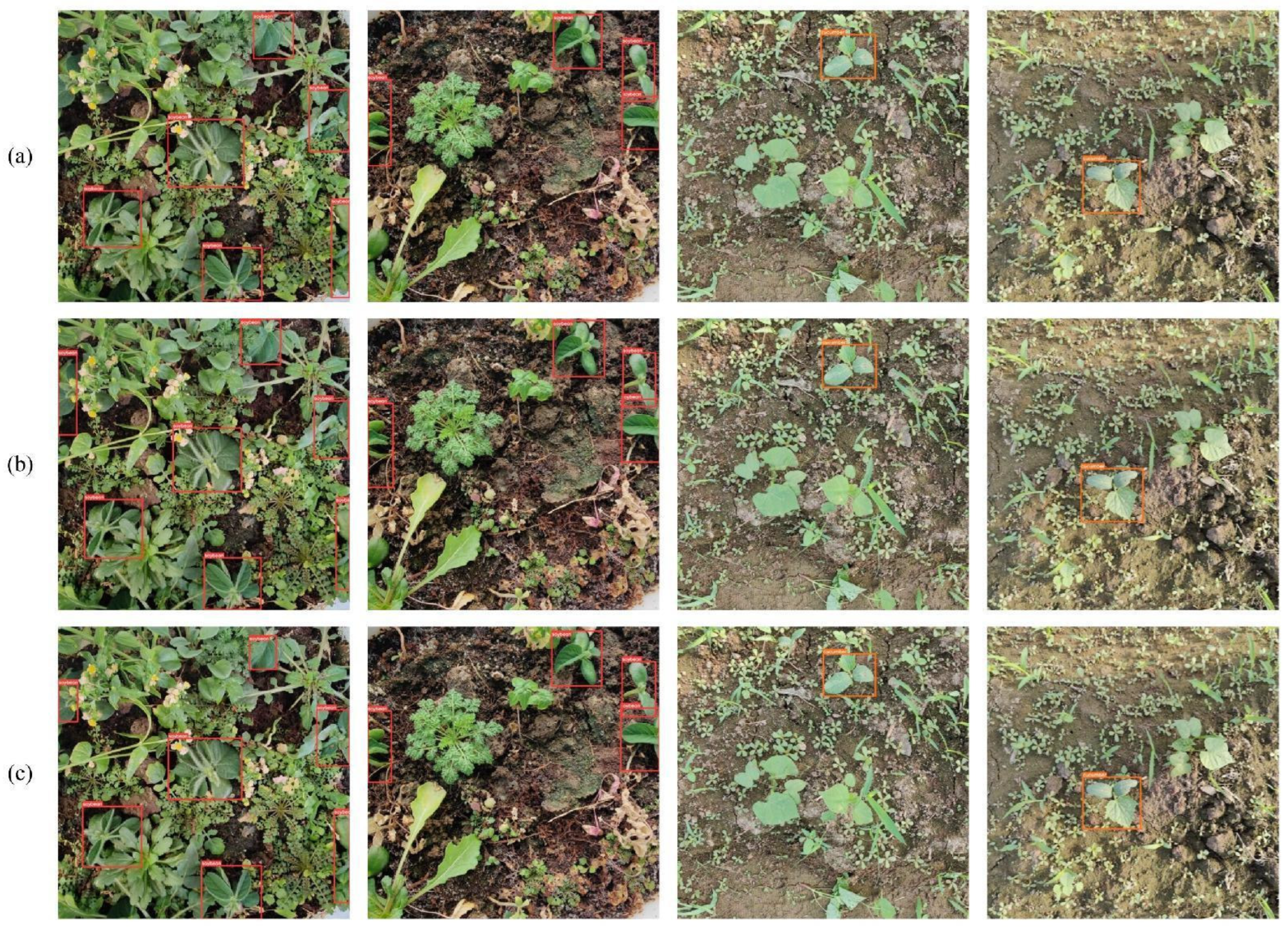
For sparsely grown crops such as cucumbers and soybeans (
Figure 13), even though the background was more complex, most of the models achieved a higher detection accuracy and produced satisfactory detection results even without any additional improvements. These findings suggested that there is no need to use strategy B for fields with low plant density during detection.
3.2. Results of the Different Transformer Detection Head
The results of eliminating the feature extraction module in the transformer mechanism are shown in
Table 4.
Benefiting from the window multi-head self-attention structure of the swim transformer, the mAP0.5 of YOLOv5ST was the highest among strategies A and B. Meanwhile, the elimination of feature blocks made the model faster. The elimination of V increased the computational speed to 164 ms·frame−1, while the computational speed after eliminating Q and V increased to 149 ms·frame−1. However, with the elimination of feature blocks, the mAP0.5 of YOLOv5ST decreased significantly. In strategy B, the computational accuracy of YOLOv5ST with feature V removed was reduced by 1.8%, and the simultaneous removal of Q and V led to a reduction in the computational accuracy of 2.8%.
The model robustness was higher for ViT with a simple structure. In strategy B, YOLOv5ViT reduced the mAP0.5 by 0.8% after eliminating V, which was smaller than that of YOLOv5ST. The simultaneous elimination of Q and V led to a reduction of 2.6% in the mAP0.5, which was similar to the reduction in YOLOv5ST. This demonstrated that the simultaneous removal of Q and V led to a reduction in the global feature extraction capability of the transformer. Although the improvement of the YOLOv5ViT computation speed was not as obvious as YOLOv5ST, which was only 23 ms·frame−1 faster on TX2, the YOLOv5ViT computation speed remained lower due to the relatively simple structure. The impact of removing the feature extraction module on the AP of cucumber was minimal. This was because the cucumber target was more prominent and the environment had fewer similar weeds without occlusions, indicating that YOLOv5 can detect this class of simple targets with a higher AP even without using the transformer mechanism.
In summary, YOLOv5ViT was the least sensitive to the effects of feature removal and had a faster speed, so YOLOv5ViT with V removed was used for further comparisons with other YOLO series models.
3.3. Comparison with Other YOLO Models
The results of each series of YOLO models are shown in
Table 5. The YOLOv5 model used in this study had smaller FLOPs than the latest YOLOv7 model, which were slightly faster to compute in the server. Since there was no structural reparameterization in YOLOv5, the computation speed in TX2 was faster than that in YOLOv7. This was the reason why we chose YOLOv5, a more mature model. The model with the transformer mechanism proposed in this paper had the same accuracy in the mAP0.5–0.95 as YOLOv7 in strategy A. Although the mAP0.5 of soybean and cucumber in strategy B was slightly lower than that of YOLOv7, both remained above 90%. The faster computation speed of our model on TX2 makes it more suitable for future embedding of the algorithm into small intelligent platforms for automated crop management applications.
4. Discussion
Accurate crop detection during the seedling stage enables the reduction in the damage inflicted by agricultural robots on crops, while simultaneously enhancing the efficiency of tasks such as fertilization and weed control. Research on crop detection using deep learning is quite extensive, such as Zou et al. [
23] who employed advanced image generation techniques and captured crop images with complex backgrounds. However, their segmentation model required additional algorithmic processing to obtain the precise location of the crops. Furthermore, their computational speed was reported as 51 ms, whereas our proposed model achieved a faster computation speed of only 16 ms. Chen et al. [
8] detected weeds in sesame fields based on the YOLOv4 detection network, but only one crop species was targeted. The same problem also occurred in the study by Hamuda [
9] et al. The study conducted by Punithavathi et al. [
24] utilized a dataset consisting of six crop species and eight weed species. However, the crops in this dataset were grown in an environment with a sparse weed presence and their computational speed was reported as 43 s, which was significantly slower compared to our model.
In our study, we also observed that the use of the single leaf labeling method resulted in a lower mAP0.5–0.95 accuracy compared to the whole crop labeling method. We speculate that this discrepancy may be attributed to the denser distribution of targets within the images when using the single leaf annotation method, which challenged the model’s ability to achieve a higher precision detection. However, the model still demonstrated a good approximation of the target position, leading to improved accuracy in mAP0.5.
In the experiments eliminating Q and V, eliminating V had the lowest influence on the accuracy, while eliminating both Q and V had the highest influence on the accuracy, as shown in
Table 4. The transformer computed the Q, K and V features of the input data, calculated the similarity weights between Q and K, and multiplied these similarity weights with V to obtain the global characteristics of V. Therefore, the results can show that the reason for the decrease in accuracy due to the simultaneous elimination of Q and V may have been that the transformer lost the ability to acquire global characteristics because the similarity weights carried the information of V (at this time, both Q and V were equal to the input data) due to our elimination of Q when calculating the similarity weights between Q and K.
In addition, we noticed that some studies used deep learning techniques for the simultaneous detection of crops and weeds. However, this paper detected crops only. This decision was made because including weeds as additional targets in environments with dense weeds would result in imbalanced data for each class, leading to decreased model accuracy. Furthermore, labeling dense weeds is an impractical task. Moreover, weed control tasks do not require the use of deep learning or machine learning for weed detection. Once the position of crops is obtained, simple threshold segmentation methods can be used to detect weeds. Finally, by utilizing the coordinates of crops, avoidance strategies can be implemented to prevent accidental harm to crops during weed control operations.
This study contributes to the detection of dense crops and the lightweight optimization of the transformer, providing accurate positioning of crop seedlings before fertilization and spraying in robotic systems. And part of the crop seedling data and the actual detection video have been made public, which can be found at the following link ‘
https://github.com/xiaozhi101/crop_detection’ (accessed on 27 April 2023). However, this study focused on the rectangular detection boxes, resulting in an insignificant improvement in wheat detection. Therefore, detection algorithms that can frame polygonal detection boxes will be investigated in the future to accurately detect crops with elongated leaves.
5. Conclusions
In this study, a target detection network was proposed for the efficient localization of crop seedlings in complex environments. The target detection network consisted of a YOLOv5 network and transformer module. First, to improve the accuracy and efficiency of the model for dense seedling detection, two labeling strategies, the whole crop labeling method (strategy A) and the single leaf labeling method (strategy B), were proposed. The results showed that the mAP0.5 could be improved from 83.1% to 84.3% using the whole crop labeling method, and from 77.3% to 81.9% for radishes (dense target). Second, the addition of the transformer module improved the mAP0.5 from 83.1% to 85% in strategy A and from 84.3% to 85.8% in strategy B, which effectively improved the detection precision of the model for complex environments and dense targets. Finally, the process of lightweight improvement of the transformer module revealed that feature extraction module V had the least impact on the features. By eliminating V, the computation speed was reduced by 1 ms·frame−1 in the server and 17 in the minicomputer TX2, and the mAP0.5 was reduced by only 0.6%, offering the possibility of real-time management of crop seedlings. Such results are particularly beneficial for complex environments and dense targets, highlighting the effectiveness of the transformer module in enhancing the performance of the model.


