
County Scale Corn Yield Estimation Based on Multi-Source Data in Liaoning Province

Abstract
:1. Introduction
2. Materials and Methods
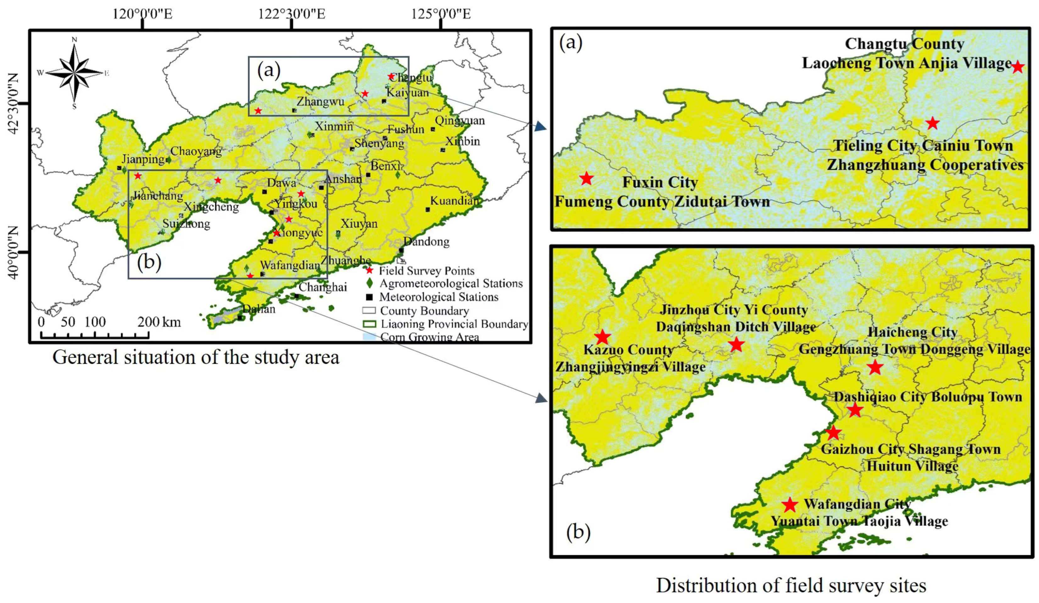
2.1. Study Area
2.2. Data Sources
2.2.1. Corn Yield Data
2.2.2. Climate Data
2.2.3. Remote Sensing Data
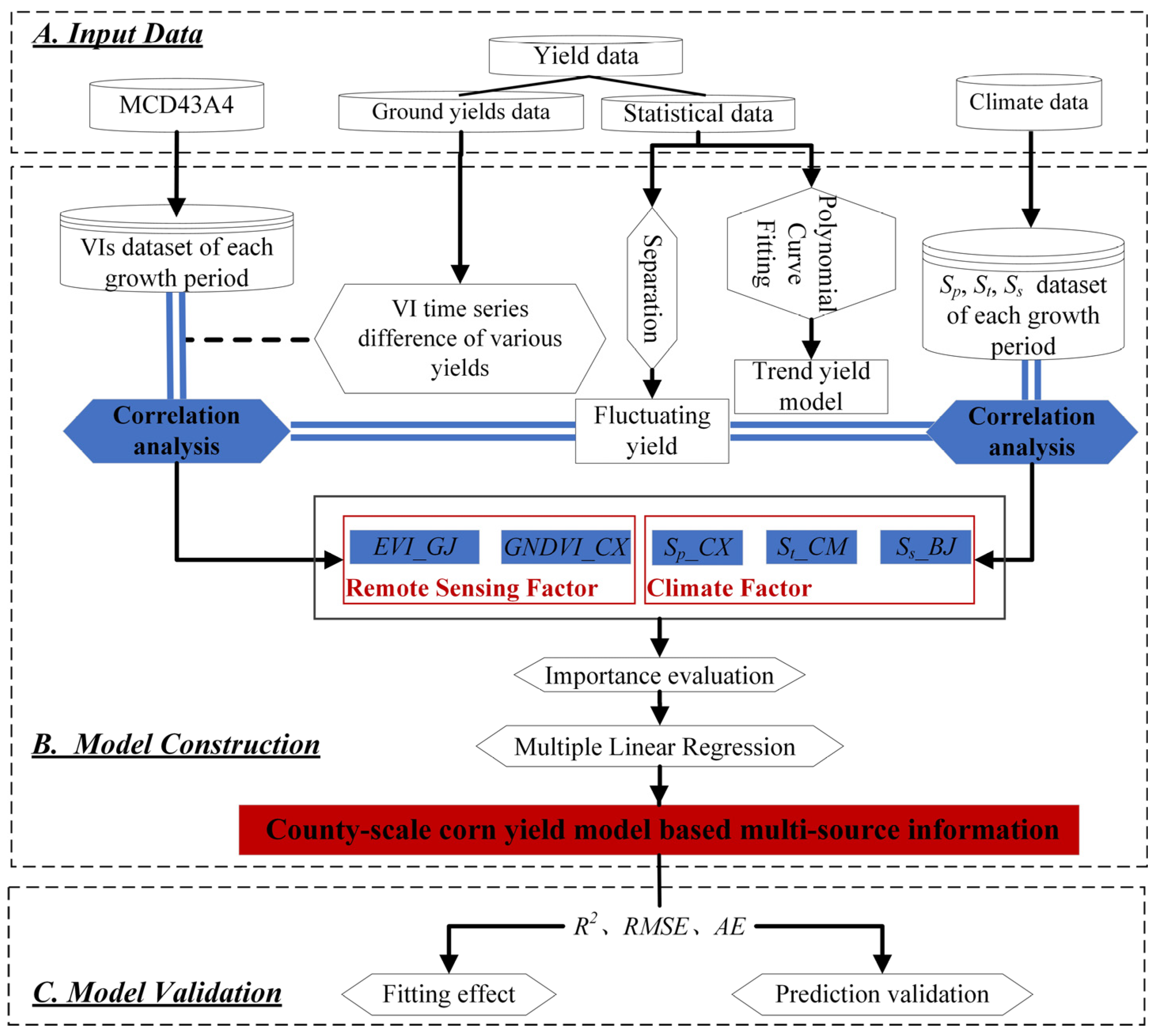
2.3. Methods
2.3.1. Factor Construction
Trend Yield
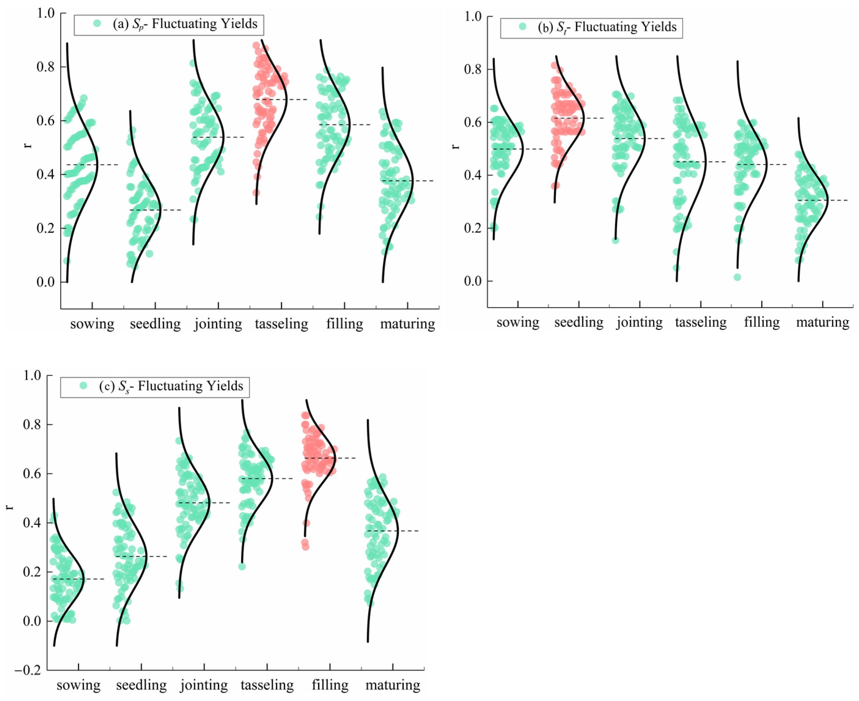
Climate Factor
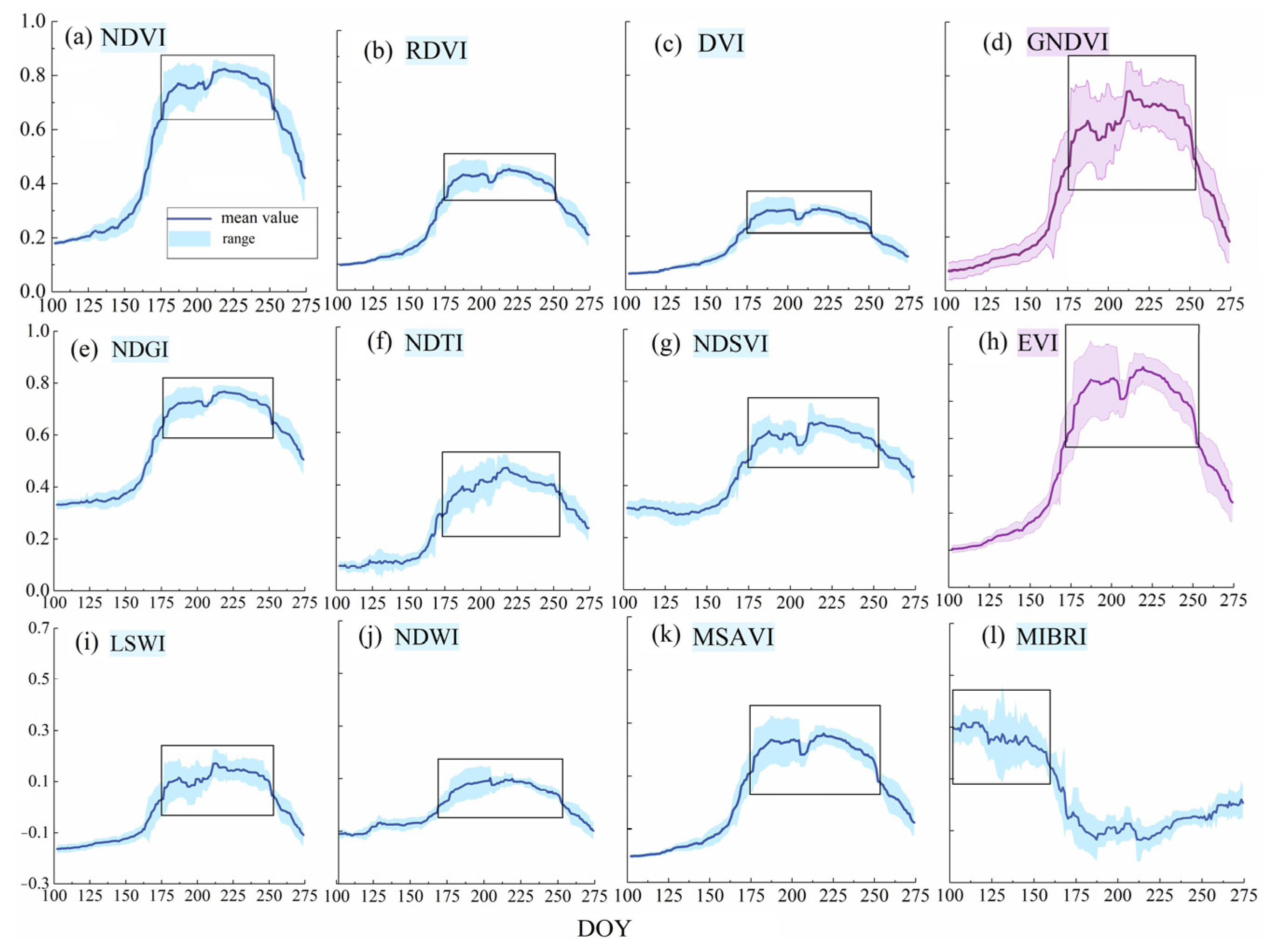
Remote Sensing Factor
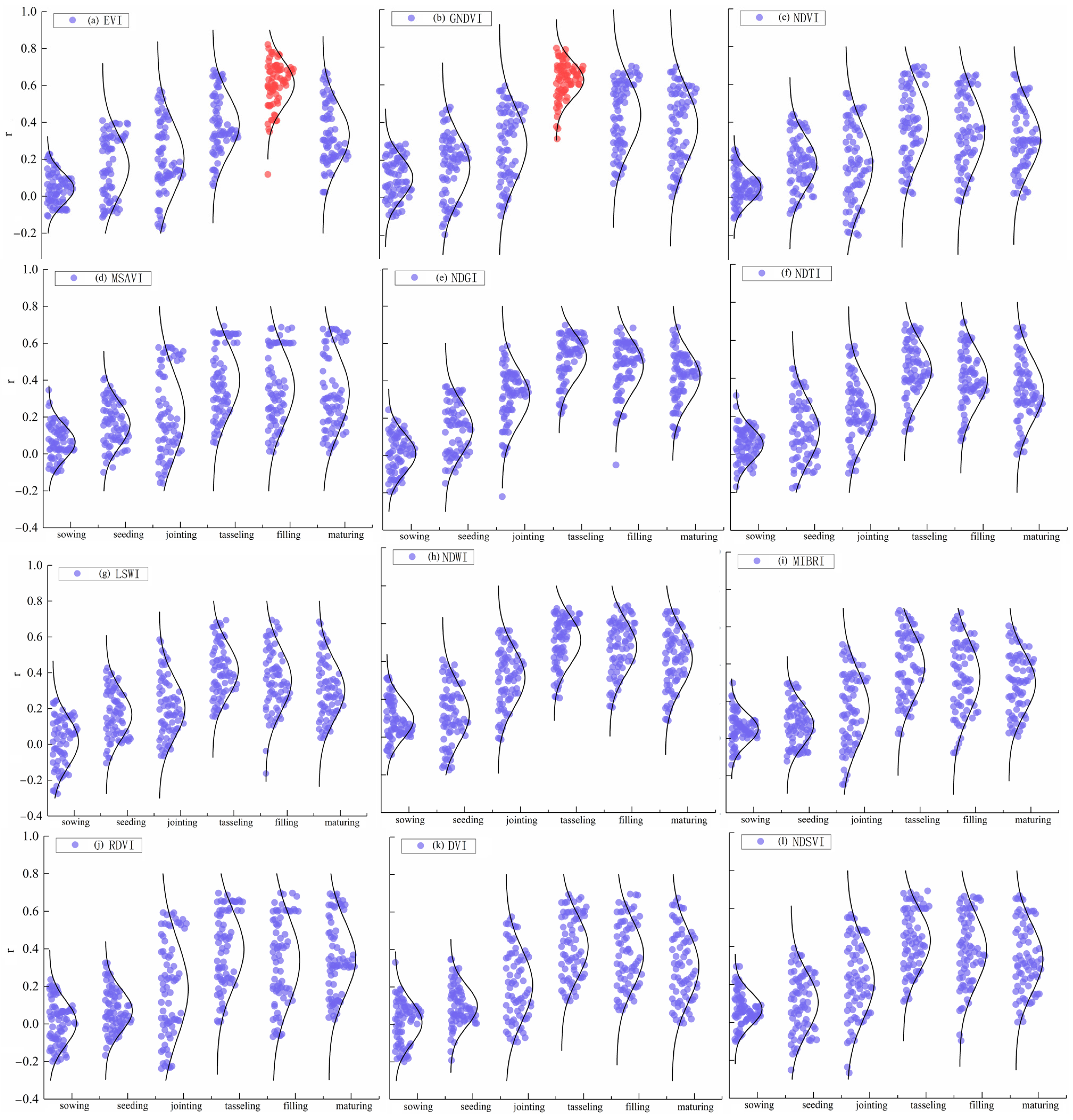
2.3.2. Climate Factor Selection Based on Correlation
2.3.3. Remote Sensing Factor Selection Based on Correlation
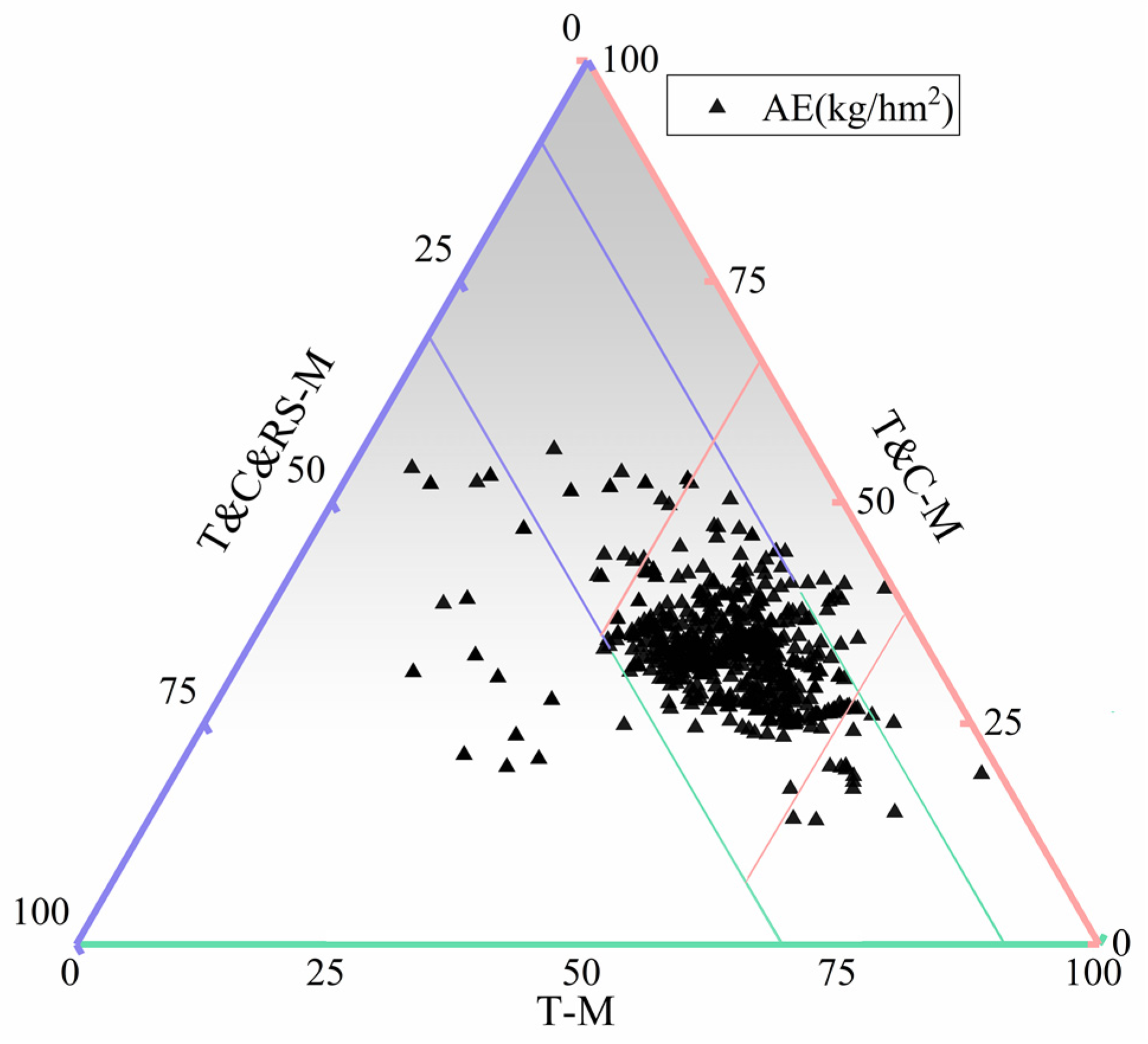
2.3.4. Factor Weight Determination for Overall Situation
3. Result
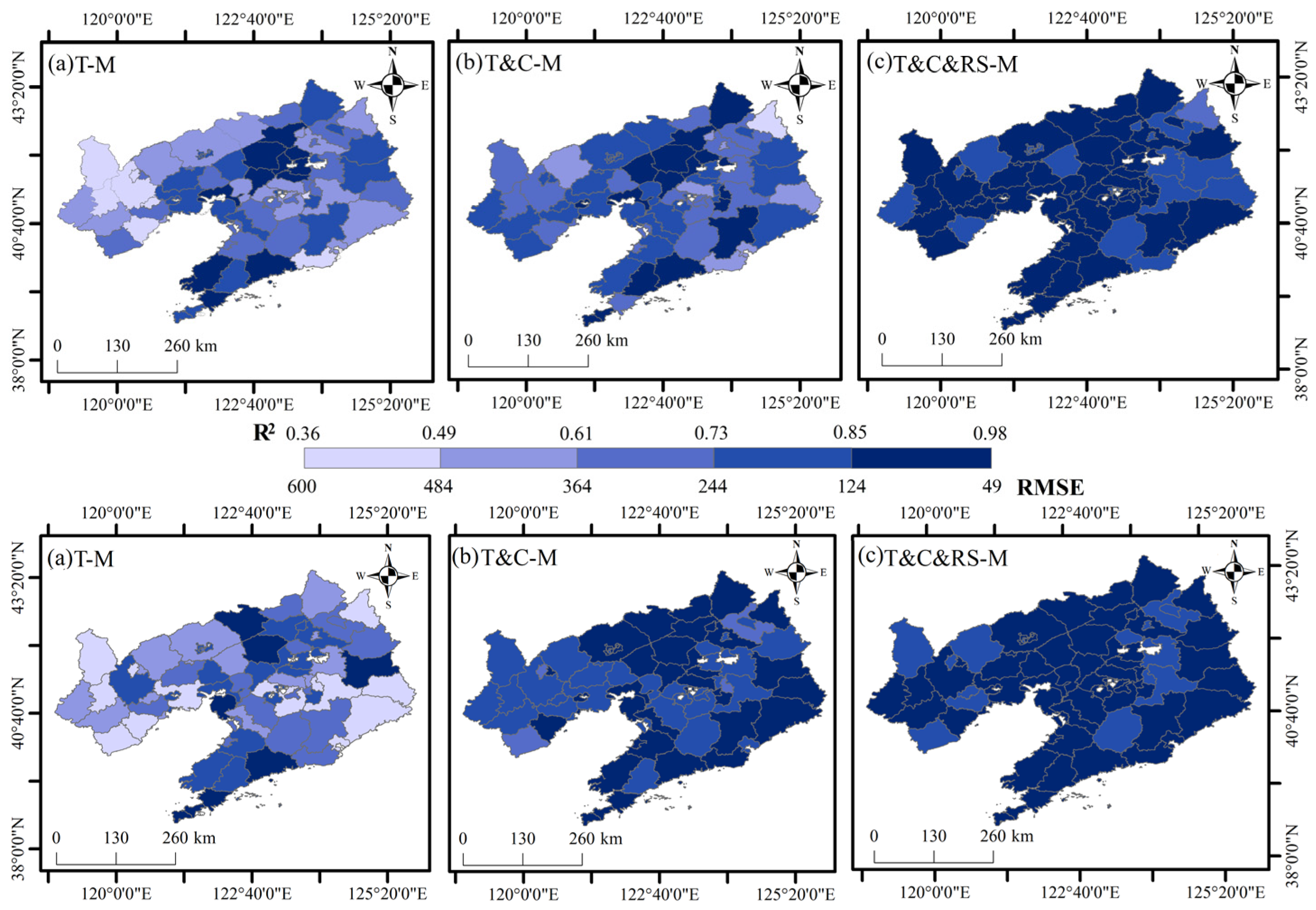
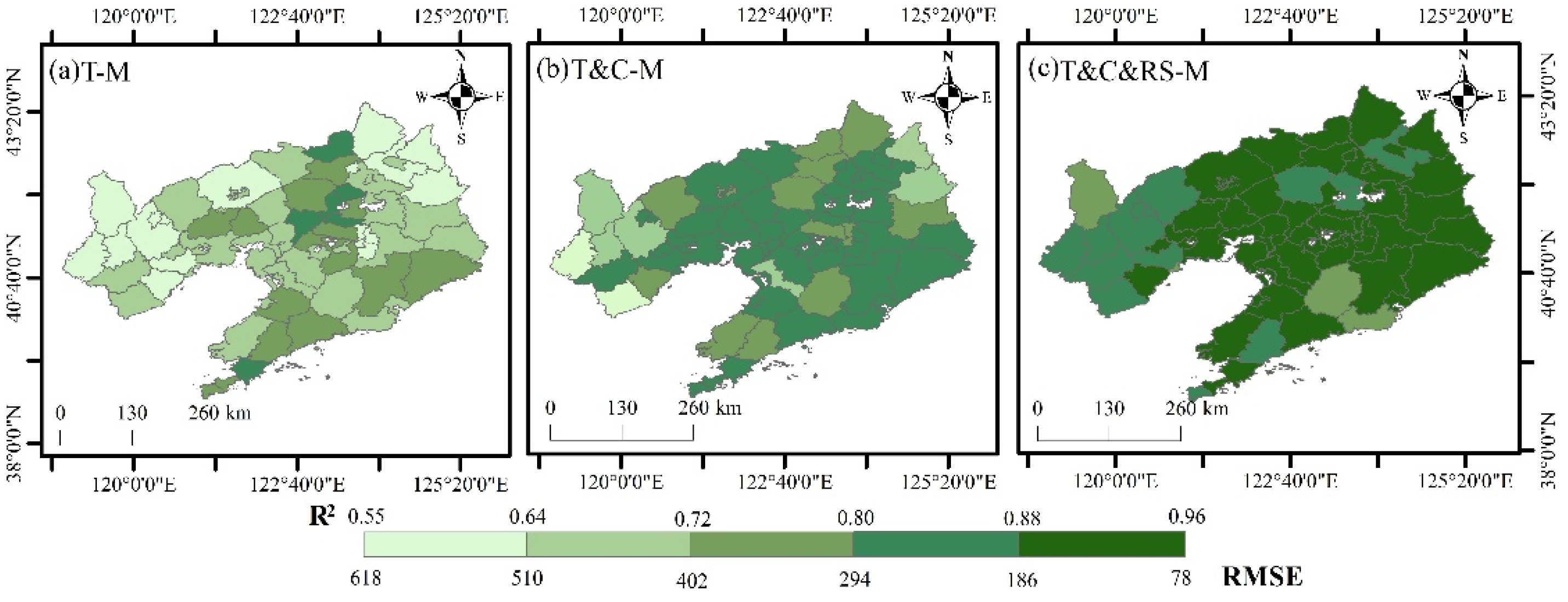
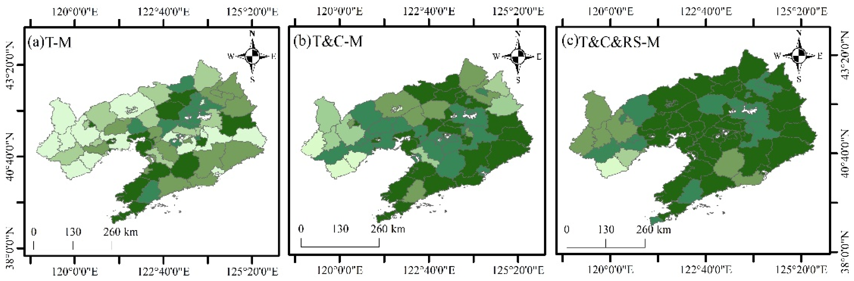
3.1. County-Level Yield Estimation Model Results
3.2. County-Level Yield Estimation Model Performance
4. Discussion
5. Conclusions
Author Contributions
Funding
Data Availability Statement
Acknowledgments
Conflicts of Interest
References
- Laborde, D.; Martin, W.; Swinnen, J.; Vos, R. COVID-19 risks to global food security. Science 2020, 369, 500–502. [Google Scholar] [CrossRef]
- Qin, X.; Feng, F.; Li, Y.; Xu, S.; Siddique, K.H.; Liao, Y. Maize yield improvements in China: Past trends and future directions. Plant Breed. 2016, 135, 166–176. [Google Scholar] [CrossRef]
- Li, S.K.; Zhao, J.R.; Dong, S.T.; Zhao, M.; Li, C.H.; Cui, Y.H.; Liu, Y.H.; Gao, J.L.; Xue, J.Q.; Wang, L.C.; et al. Advances and prospects of maize cultivation in China. Sci. Agric. Sin. 2017, 50, 1941–1959. [Google Scholar]
- Ma, D.L.; Xie, R.Z.; Yu, X.F.; Li, S.K.; Gao, J.L. Historical trends in maize morphology from the 1950s to the 2010s in China. J. Integr. Agric. 2022, 21, 2159–2167. [Google Scholar] [CrossRef]
- Assefa, Y.; Prasad, P.V.V.; Carter, P.; Hinds, M.; Bhalla, G.; Schon, R.; Jeschke, M.; Paszkiewicz, S.; Ciampitti, I.A. A New Insight into Corn Yield: Trends from 1987 through 2015. Crop Sci. 2017, 57, 2799–2811. [Google Scholar] [CrossRef]
- Li, Y.; Guan, K.; Yu, A.; Peng, B.; Zhao, L.; Li, B.; Peng, J. Toward building a transparent statistical model for improving crop yield prediction: Modeling rainfed corn in the US. Field Crop. Res. 2019, 234, 55–65. [Google Scholar] [CrossRef]
- Brisson, N.; Gary, C.; Justes, E.; Roche, R.; Mary, B.; Ripoche, D.; Zimmer, D.; Sierra, J.; Bertuzzi, P.; Burger, P.; et al. An overview of the crop model STICS. Eur. J. Agron. 2003, 18, 309–332. [Google Scholar] [CrossRef]
- Brisson, N.; Beaudoin, N.; Mary, B.; Launay, M. Conceptual Basis, Formalisations and Parameterization of the STICS Crop Model; Quae: Versailles, France, 2009; pp. 1–298. [Google Scholar]
- Jones, J.W.; Hoogenboom, G.; Porter, C.H.; Boote, K.J.; Batchelor, W.D.; Hunt, L.A.; Wilkens, P.W.; Singh, U.; Gijsman, A.J.; Ritchie, J.T. The DSSAT cropping system model. Eur. J. Agron. 2003, 18, 235–265. [Google Scholar] [CrossRef]
- Liu, K.; Harrison, M.T.; Yan, H.; Liu, D.; Meinke, H.; Hoogenboom, G.; Wang, B.; Peng, B.; Guan, K.; Jaegermeyr, J.; et al. Silver lining to a climate crisis in multiple prospects for alleviating crop waterlogging under future climates. Nat. Commun. 2023, 14, 765. [Google Scholar] [CrossRef]
- Allard, D.W.; Hendrik, B.; Davide, F.; Sander, J.; Rob, K.; Daniel, K.; Iwan, S.; Raymond, D.; Wijngaart, K.D. 25 years of the WOFOST cropping systems model. Agric. Syst. 2019, 168, 154–167. [Google Scholar]
- Sun, Y.; Zhang, S.; Tao, F.; Aboelenein, R.; Amer, A. Improving Winter Wheat Yield Forecasting Based on Multi-Source Data and Machine Learning. Agriculture 2022, 12, 571. [Google Scholar] [CrossRef]
- Jiang, H.; Hu, H.; Zhong, R.; Xu, J.; Xu, J.; Huang, J.; Wang, S.; Ying, Y.; Lin, T. A deep learning approach to conflating heterogeneous geospatial data for corn yield estimation: A case study of the US Corn Belt at the county level. Glob. Chang. Biol. 2020, 26, 1754–1766. [Google Scholar] [CrossRef]
- Rosenzweig, C.; Elliott, J.; Deryng, D.; Ruane, A.C.; Müller, C.; Arneth, A.; Boote, K.J.; Folberth, C.; Glotter, M.; Khabarov, N.; et al. Assessing agricultural risks of climate change in the 21st century in a global gridded crop model intercomparison. Proc. Natl. Acad. Sci. USA 2014, 111, 3268–3273. [Google Scholar] [CrossRef] [PubMed]
- Basso, B.; Liu, L. Seasonal crop yield forecast: Methods, applications, and accuracies. Adv. Agron. 2019, 154, 201–255. [Google Scholar]
- Niedbała, G.; Nowakowski, K.; Rudowicz-Nawrocka, J.; Piekutowska, M.; Weres, J.; Tomczak, R.J.; Tyksiński, T.; Álvarez Pinto, A. Multicriteria Prediction and Simulation of Winter Wheat Yield Using Extended Qualitative and Quantitative Data Based on Artificial Neural Networks. Appl. Sci. 2019, 9, 2773. [Google Scholar] [CrossRef]
- Panek, E.; Gozdowski, D. Relationship between MODIS Derived NDVI and Yield of Cereals for Selected European Countries. Agronomy 2021, 11, 340. [Google Scholar] [CrossRef]
- Ruonan, Q.; Xing, L.; Ge, H.; Jingfeng, X.; Xin, M.; Wei, G. Monitoring drought impacts on crop productivity of the U.S. Midwest with solar-induced fluorescence: GOSIF outperforms GOME-2 SIF and MODIS NDVI, EVI, and NIRv. Agric. For. Meteorol. 2022, 323, 109038. [Google Scholar]
- Byjesh, K.; Kumar, S.N.; Aggarwal, P.K. Simulating impacts, potential adaptation and vulnerability of maize to climate change in India. Mitig. Adapt. Strateg. Glob. Chang. 2021, 15, 413–431. [Google Scholar] [CrossRef]
- Gonzalo, R.; Juan, P.M.; Fatima, A.T.; Réka, H.; Kenneth, G.C.; Patricio, G. Climate and agronomy, not genetics, underpin recent maize yield gains in favorable environments. Proc. Natl. Acad. Sci. USA 2022, 119, 4. [Google Scholar]
- Lobell, D.B.; Schlenker, W.; Costa-Roberts, J. Climate trends and global crop production since 1980. Science 2011, 333, 616–620. [Google Scholar] [CrossRef] [PubMed]
- Xiong, W.; Asseng, S.; Hoogenboom, G.; Hernandez-Ochoa, I.; Robertson, R.; Sonder, K.; Pequeno, D.; Reynolds, M.; Gerard, B. Different uncertainty distribution between high and low latitudes in modelling warming impacts on wheat. Nat. Food 2019, 1, 63–69. [Google Scholar] [CrossRef]
- Zhang, L.; Zhang, Z.; Luo, Y.; Cao, J.; Tao, F. Combining Optical, Fluorescence, Thermal Satellite, and Environmental Data to Predict County-Level Maize Yield in China Using Machine Learning Approaches. Remote Sens. 2020, 12, 21. [Google Scholar] [CrossRef]
- Juan, C.; Zhao, Z.; Fulu, T.; Liangliang, Z.; Yuchuan, L.; Jing, Z.; Jichong, H.; Jun, X. Integrating Multi-Source Data for Rice Yield Prediction across China using Machine Learning and Deep Learning Approaches. Agric. For. Meteorol. 2021, 297, 0168–1923. [Google Scholar]
- Teal, R.K.; Tubana, B.; Girma, K.; Freeman, K.W.; Arnall, D.B.; Walsh, O.; Raun, W.R. In-season prediction of corn grain yield potential using normalized difference vegetation index. Agron. J. 2006, 98, 1488–1494. [Google Scholar] [CrossRef]
- Huang, S.; Tang, L.; Hupy, J.P.; Wang, Y.; Shao, G. A commentary review on the use of normalized difference vegetation index (NDVI) in the era of popular remote sensing. J. For. Res. 2021, 32, 1–6. [Google Scholar] [CrossRef]
- Saad El Imanni, H.; El Harti, A.; El Iysaouy, L. Wheat Yield Estimation Using Remote Sensing Indices Derived from Sentinel-2 Time Series and Google Earth Engine in a Highly Fragmented and Heterogeneous Agricultural Region. Agronomy 2022, 12, 2853. [Google Scholar] [CrossRef]
- Son, N.T.; Chen, C.F.; Chen, C.R.; Minh, V.Q.; Trung, N.H. A comparative analysis of multitemporal MODIS EVI and NDVI data for large-scale rice yield estimation. Agric. For. Meteorol. 2014, 197, 52–64. [Google Scholar] [CrossRef]
- Bolton, D.K.; Friedl, M.A. Forecasting crop yield using remotely sensed vegetation indices and crop phenology metrics. Agric. For. Meteorol. 2013, 173, 74–84. [Google Scholar] [CrossRef]
- Li, Z.; Ding, L.; Xu, D. Exploring the potential role of environmental and multi-source satellite data in crop yield prediction across Northeast China. Sci. Total Environ. 2022, 815, 152880. [Google Scholar] [CrossRef] [PubMed]
- García-Martínez, H.; Flores-Magdaleno, H.; Ascencio-Hernández, R.; Khalil-Gardezi, A.; Tijerina-Chávez, L.; Mancilla-Villa, O.R.; Vázquez-Peña, M.A. Corn Grain Yield Estimation from Vegetation Indices, Canopy Cover, Plant Density, and a Neural Network Using Multispectral and RGB Images Acquired with Unmanned Aerial Vehicles. Agriculture 2020, 10, 277. [Google Scholar] [CrossRef]
- Kamir, E.; Waldner, F.; Hochman, Z. Estimating wheat yields in Australia using climate records, satellite image time series and machine learning methods. ISPRS J. Photogramm. Remote Sens. 2020, 160, 124–135. [Google Scholar] [CrossRef]
- Peng, B.; Guan, K.; Zhou, W.; Jiang, C.; Frankenberg, C.; Sun, Y.; He, L.; Köhler, P. Assessing the benefit of satellite-based Solar-Induced Chlorophyll Fluorescence in crop yield prediction. Int. J. Appl. Earth Obs. Geoinf. 2020, 90, 102126. [Google Scholar] [CrossRef]
- Mateo-Sanchis, A.; Piles, M.; Muñoz-Marí, J.; Adsuara, J.E.; Pérez-Suay, A.; Camps-Valls, G. Synergistic integration of optical and microwave satellite data for crop yield estimation. Remote Sens. Environ. 2019, 234, 111460. [Google Scholar] [CrossRef] [PubMed]
- Kouadio, L.; Newlands, N.K.; Davidson, A.; Zhang, Y.; Chipanshi, A. Assessing the Performance of MODIS NDVI and EVI for Seasonal Crop Yield Forecasting at the Ecodistrict Scale. Remote Sens. 2014, 6, 10193–10214. [Google Scholar] [CrossRef]
- Tan, F.Y.; He, L.; Lyu, H.Q.; Song, Y.B.; Cheng, L.; Hou, Y.Y. Application of agricultural drought index based on Run Theory for the assessment of yield loss in spring maize owing to drought in Liaoning Province. Chin. J. Eco-Agric. 2020, 28, 191–199. [Google Scholar]
- Zhang, Q.; Zhang, J.; Wang, C.; Liang, C.; Deng, H.Y. Risk early warning of maize drought disaster in Northwestern Liaoning Province. China Nat. Hazards 2014, 72, 701–710. [Google Scholar] [CrossRef]
- You, N.; Dong, J.; Huang, J.; Du, G.; Zhang, G.; He, Y.; Yang, T.; Di, Y.; Xiao, X. The 10-m crop type maps in Northeast China during 2017–2019. Sci. Data 2021, 8, 41. [Google Scholar] [CrossRef]
- Ju, X.; Tu, Q.; Li, Q. Discussion on the climatological calculation of solar radiation. Trans. Atmos. Sci. 2005, 28, 516–521. [Google Scholar]
- Feng, Y.; Cui, N.; Hao, W.; Gao, L.; Gong, D. Estimation of soil temperature from meteorological data using different machine learning models. Geoderma 2019, 338, 67–77. [Google Scholar] [CrossRef]
- Zhao, Y.; Qi, J.; Wang, F.; Li, L.; Lu, J. Climate Suitability and Annual Assessment of Spring Maize During Full Breeding Period in Liaoning Province. Geogr. Sci. 2020, 40, 1210–1220. [Google Scholar]
- Strahler, A.H.; Muller, J.P.; Lucht, W.; Schaaf, C.B.; Tsang, T.; Gao, F.; Li, X.; Lewis, P.; Barnsley, M.J. MODIS BRDF/albedo product: Algorithm theoretical basis document version 5.0. MODIS Doc. 1999, 23, 42–47. [Google Scholar]
- Zhang, M.; Zhang, M.; Yang, H.; Jin, Y.; Zhang, X.; Liu, H. Mapping Regional Soil Organic Matter Based on Sentinel-2A and MODIS Imagery Using Machine Learning Algorithms and Google Earth Engine. Remote Sens. 2021, 13, 2934. [Google Scholar] [CrossRef]
- Dineshkumar, C.; Nitheshnirmal, S.; Bhardwaj, A.; Priyadarshini, K.N. Phenological Monitoring of Paddy Crop Using Time Series MODIS Data. Proceedings 2019, 24, 19. [Google Scholar]
- Yin, L.; You, N.; Zhang, G.; Huang, J.; Dong, J. Optimizing Feature Selection of Individual Crop Types for Improved Crop Mapping. Remote Sens. 2020, 12, 162. [Google Scholar] [CrossRef]
- Chen, C.; Zhu, X.; Cai, Y.; Guo, H. A hybrid yield estimation model based on the trend yield model and remote sensing correction yield model. Sci. Agric. Sin. 2017, 50, 1792–1801. [Google Scholar]
- Zhao, D.; Wang, Y.; Ren, C.; Ma, X.; Xu, Y.; Chen, W. Comparative analysis of three fitting methods of rice trend yield. Chin. J. Eco-Agric. 2017, 25, 345–355. [Google Scholar]
- Yang, X.; Lin, E.; Ma, S.; Ju, H.; Guo, L.; Xiong, W.; Li, Y.; Xu, Y. Adaptation of agriculture to warming in Northeast China. Clim. Chang. 2007, 84, 45–58. [Google Scholar] [CrossRef]
- Patil, M.E.; Roshini, M.; Chitrarupa, M.; Laxmaiah, B.; Arun, S.; Thiagarajan, R. A Hybrid Approach for Crop Yield Prediction using Supervised Machine Learning. In Proceedings of the 2022 8th International Conference on Smart Structures and Systems (ICSSS), Chennai, India, 21–22 April 2022; pp. 1–6. [Google Scholar]
- Hou, Y.; Zhang, Y.; Wang, L.; Lv, H.; Song, Y. Climatic suitability model for spring maize in Northeast China. Chin. J. Appl. Ecol. 2013, 24, 3207–3212. [Google Scholar]
- Masoudi, M. Estimation of the spatial climate comfort distribution using tourism climate index (TCI) and inverse distance weighting (IDW)(case study: Fars Province, Iran). Arab. J. Geosci. 2021, 14, 363. [Google Scholar] [CrossRef]
- Khouni, I.; Louhichi, G.; Ghrabi, A. Use of GIS based Inverse Distance Weighted interpolation to assess surface water quality: Case of Wadi El Bey, Tunisia. Environ. Technol. Innov. 2021, 24, 101892. [Google Scholar] [CrossRef]
- Xin, N. China Agrometeorology; China Agriculture Press: Beijing, China, 1999. [Google Scholar]
- Song, Y.; Wang, J.; Yang, F. Meteorological Services for Food Security; China Meteorological Press: Beijing, China, 2006. [Google Scholar]
- Su, Z.; Liu, Z.; Bai, F.; Zhang, Z.; Sun, S.; Huang, Q.; Liu, T.; Liu, X.; Yang, X. Cultivar selection can increase yield potential and resource use efficiency of spring maize to adapt to climate change in Northeast China. J. Integr. Agric. 2021, 20, 371–382. [Google Scholar] [CrossRef]
- Zhao, Y.; Xiao, D.; Bai, H.; Tang, J.; Liu, D. Future Projection for Climate Suitability of Summer Maize in the North China Plain. Agriculture 2022, 12, 348. [Google Scholar] [CrossRef]
- Rouse, J.W.; Haas, R.H.; Schell, J.A.; Deering, D.W. Monitoring vegetation systems in the Great Plains with ERTS. NASA Spec. Publ. 1974, 351, 309. [Google Scholar]
- Huete, A.; Didan, K.; Miura, T.; Rodriguez, E.P.; Gao, X.; Ferreira, L.G. Overview of the radiometric and biophysical performance of the MODIS vegetation indices. Remote Sens. Environ. 2002, 83, 195–213. [Google Scholar] [CrossRef]
- Qi, J.; Chehbouni, A.; Huete, A.R.; Kerr, Y.H.; Sorooshian, S. A modified soil adjusted vegetation index. Remote Sens. Environ. 1994, 48, 119–126. [Google Scholar] [CrossRef]
- Broge, N.H.; Leblanc, E. Comparing prediction power and stability of broadband and hyperspectral vegetation indices for estimation of green leaf area index and canopy chlorophyll density. Remote Sens. Environ. 2001, 76, 156–172. [Google Scholar] [CrossRef]
- Gitelson, A.A.; Kaufman, Y.J.; Merzlyak, M.N. Use of a green channel in remote sensing of global vegetation from EOS-MODIS. Remote Sens. Environ. 1996, 58, 289–298. [Google Scholar] [CrossRef]
- Roujean, J.L.; Breon, F.M. Estimating PAR absorbed by vegetation from bidirectional reflectance measurements. Remote Sens. Environ. 1995, 51, 375–384. [Google Scholar] [CrossRef]
- Xiao, X.; Boles, S.; Liu, J.; Zhuang, D.; Liu, M. Characterization of forest types in Northeastern China, using multi-temporal SPOT-4 VEGETATION sensor data. Remote Sens. Environ. 2002, 82, 335–348. [Google Scholar] [CrossRef]
- Qi, J.; Marsett, R.; Heilman, P.; Bieden-bender, S.; Moran, S.; Goodrich, D.; Weltz, M. RANGES improves satellite-based information and land cover assessments in southwest United States. Eos Trans. Am. Geophys. Union 2002, 83, 601–606. [Google Scholar] [CrossRef]
- Gao, L.; Zhang, C.; Yun, W.; Ji, W.; Ma, J.; Wang, H.; Li, C.; Zhu, D.H. Mapping crop residue cover using Adjust Normalized Difference Residue Index based on Sentinel-2 MSI data. Soil Tillage Res. 2022, 220, 105374. [Google Scholar] [CrossRef]
- Meyer, G.E.; Neto, J.C. Verification of color vegetation indices for automated crop imaging applications. Comput. Electron. Agric. 2008, 63, 282–293. [Google Scholar] [CrossRef]
- Gao, B.C. Normalized difference water index for remote sensing of vegetation liquid water from space. Imaging Spectrom. Int. Soc. Opt. Photonics 1995, 2480, 225–236. [Google Scholar]
- Datta, D.; Chandra, S.; Nath, C.P.; Kar, G.; Ghosh, S.; Chaturvedi, S.; Bhatnagar, A.; Singh, G.; Singh, V. Soil-plant water dynamics, yield, quality and profitability of spring sweet corn under variable irrigation scheduling, crop establishment and moisture conservation practices. Field Crop. Res. 2022, 279, 108450. [Google Scholar] [CrossRef]
- Cakir, R. Effect of water stress at different development stages on vegetative and reproductive growth of corn. Field Crop. Res. 2004, 89, 1–16. [Google Scholar] [CrossRef]
- Shaw, R.H. Crop Reactions to Water and Temperature Stresses in Humid, Temperate Climates; CRC Press: Boca Raton, FL, USA, 2019; pp. 49–65. [Google Scholar]
- Coelho, D.T.; Dale, R.F. An Energy-Crop Growth Variable and Temperature Function for Predicting Corn Growth and Development: Planting to Silking 1. Agron. J. 1980, 72, 503–510. [Google Scholar] [CrossRef]
- Alessi, J.; Power, J.F. Corn emergence in relation to soil temperature and seeding depth 1. Agron. J. 1971, 63, 717–719. [Google Scholar] [CrossRef]
- Walne, C.H.; Reddy, K.R. Temperature Effects on the Shoot and Root Growth, Development, and Biomass Accumulation of Corn (Zea mays L.). Agriculture 2022, 12, 443. [Google Scholar] [CrossRef]
- Warrington, I.J.; Kanemasu, E.T. Corn growth response to temperature and photoperiod I. Seedling emergence, tassel initiation, and anthesis 1. Agron. J. 1983, 75, 749–754. [Google Scholar] [CrossRef]
- Xu, C.; Zhang, P.; Wang, Y.; Luo, N.; Tian, B.; Liu, X.; Wang, P.; Huang, S. Grain yield and grain moisture associations with leaf, stem and root characteristics in maize. J. Integr. Agric. 2022, 21, 1941–1951. [Google Scholar] [CrossRef]
- Fang, H.; Liang, S.; Hoogenboom, G. Integration of MODIS LAI and vegetation index products with the CSM–CERES–Maize model for corn yield estimation. Int. J. Remote Sens. 2011, 32, 1039–1065. [Google Scholar] [CrossRef]
- Oliveira, M.F.d.; Ortiz, B.V.; Morata, G.T.; Jiménez, A.F.; Rolim, G.d.S.; Silva, R.P.d. Training Machine Learning Algorithms Using Remote Sensing and Topographic Indices for Corn Yield Prediction. Remote Sens. 2022, 14, 6171. [Google Scholar] [CrossRef]
- Yuan, M.; Ekici, A.; Lu, Z.; Monteiro, R. Dimension reduction and coefficient estimation in multivariate linear regression. J. R. Stat. Soc. Ser. B Stat. Methodol. 2007, 69, 329–346. [Google Scholar] [CrossRef]
- Johnson, D.M.; Rosales, A.; Mueller, R.; Reynolds, C.; Frantz, R.; Anyamba, A.; Pak, E.; Tucker, C. USA Crop Yield Estimation with MODIS NDVI: Are Remotely Sensed Models Better than Simple Trend Analyses? Remote Sens. 2021, 13, 4227. [Google Scholar] [CrossRef]
- Fu, Z.; Jiang, J.; Gao, Y.; Krienke, B.; Wang, M.; Zhong, K.; Cao, Q.; Tian, Y.; Zhu, Y.; Cao, W.; et al. Wheat Growth Monitoring and Yield Estimation based on Multi-Rotor Unmanned Aerial Vehicle. Remote Sens. 2020, 12, 508. [Google Scholar] [CrossRef]
- Cao, J.; Zhang, Z.; Tao, F.; Zhang, L.; Luo, Y.; Han, J.; Li, Z. Identifying the Contributions of Multi-Source Data for Winter Wheat Yield Prediction in China. Remote Sens. 2020, 12, 750. [Google Scholar] [CrossRef]
- Zhao, J.; Pan, F.; Xiao, X.; Hu, L.; Wang, X.; Yan, Y.; Zhang, S.; Tian, B.; Yu, H.; Lan, Y. Summer Maize Growth Estimation Based on Near-Surface Multi-Source Data. Agronomy 2023, 13, 532. [Google Scholar] [CrossRef]


| Category | Name | Spatial Resolution | Temporal Resolution | Source |
|---|---|---|---|---|
| Remote Sensing data | MCD43A4 (Version 6) | 500 m | Daily | Download on the Google Earth Engine (Dataset Provider: NASA LP DAAC at the USGS EROS Center) |
| Crop Type Cover Products | 10 m | Year | Provided by You et al. [38] (https://doi.org/10.6084/m9.figshare.13090442, accessed on 16 October 2020) | |
| Climate data | Precipitation data | Weather Stations | Daily | China Meteorological Administration (http://data.cma.cn, accessed on 20 October 2021) |
| Temperature data | Weather Stations | Daily | Same as Above | |
| Sunshine data | Weather Stations | Daily | Same as Above | |
| Corn Yield data | County-level Corn Yield in Liaoning | County | Year | County Statistical Yearbook |
| Measured Yield | Field Scale | Year | Provided by Liaoning Academy of Agricultural Sciences |
| Fertility Stage | Tl | To | Th | Kc | b |
|---|---|---|---|---|---|
| Sowing Stage | 10 | 17 | 25 | 0.354 | 4.77 |
| Seedling Stage | 14 | 26 | 30 | 0.773 | 5.08 |
| Jointing Stage | 17 | 26 | 33 | 0.773 | 5.08 |
| Tasseling Stage | 16 | 23 | 35 | 1.288 | 5.16 |
| Filling Stage | 14 | 22 | 32 | 1.167 | 5.21 |
| Maturing Stage | 13 | 20 | 30 | 0.615 | 5.24 |
| Vegetation Index | Equation |
|---|---|
| Normalized Differenced Vegetation Index, NDVI [56] | |
| The Enhanced Vegetation Index, EVI [57] | |
| Modified Soil Adjusted Vegetation Index, MSAVI [58] | |
| Differenced Vegetation Index, DVI [59] | |
| Green Normalized Differenced Vegetation Index, GNDVI [60] | |
| Renormalized Differenced Vegetation Index, RDVI [61] | |
| Land Surface Water Index, LSWI [62] | |
| Normalized Difference Senescent Vegetation Index, NDSVI [63] | |
| Normalized Difference Tillage Index, NDTI [64] | |
| Normalized Difference Greenness Index, NDGI [65] | |
| Normalized Difference Water Index, NDWI [66] | |
| Mid-IR Bispectral Index, MIRBI [67] |
| Coefficient | a | b | c | d | e | k | Coefficient | a | b | c | d | e | k | ||
|---|---|---|---|---|---|---|---|---|---|---|---|---|---|---|---|
| Eastern Liaoning | Shuncheng | 195.92 | −273.42 | 91.08 | 250.44 | 149.19 | 199.35 | Western Liaoning | Taihe | −312.18 | 189.83 | −491.35 | 213.84 | 107.79 | 162.99 |
| Fushun | −222.51 | −307.47 | 32.15 | 242.09 | 141.24 | 192.99 | Heishan | −213.74 | 177.76 | −438.9 | 188.75 | 88.75 | 151 | ||
| Pingshan | −231.53 | 283.17 | −216.48 | 357.15 | 213.44 | 250.75 | Yixian | −359.28 | 305.47 | −366.92 | 326.25 | 226.25 | −261.44 | ||
| Xihu | 164.47 | 350.68 | −45.4 | 134.69 | 47.83 | 115.26 | Linghai | 303.36 | 5.86 | −216.48 | −176.29 | 203.36 | 242.69 | ||
| Xinbin | −214.01 | −116.98 | 202.77 | 283.36 | 183.66 | 26.93 | Beizhen | 480.16 | 189.7 | −274.9 | −358.17 | 258.17 | −286.54 | ||
| Qingyuan | 206.21 | 263.11 | −38.22 | −309.51 | 216.72 | 50.85 | Haizhou | −248.37 | 23.97 | 291.27 | 274.42 | 180.11 | −219.53 | ||
| Mingshan | −175.99 | 28.18 | −74.53 | 300.79 | 220.07 | 240.58 | Xinqiu | −157.99 | 130.44 | −104.5 | −253.85 | 151.48 | 201.18 | ||
| Nanfen | 197.08 | 264.25 | −8.54 | −251.78 | 97.08 | 157.66 | Taiping | −203.71 | 136.22 | −98.37 | 138.25 | 63.94 | 109.55 | ||
| Benxi | −203.81 | 256.73 | −104.64 | 313.92 | 242.22 | 259.14 | Qinghemen | 206.13 | 163.69 | −188.32 | 143.29 | 43.64 | −114.59 | ||
| Huanren | −176.49 | 173.84 | 52.03 | 164.7 | 65.86 | 132.69 | Xihe | 203.38 | 446.62 | 170.44 | 331.7 | −208.57 | 241.25 | ||
| Zhenan | −183.9 | 363.62 | 8.54 | 20.96 | −257.36 | 340.33 | Fumeng | 252.56 | 268.22 | 352.01 | 185.06 | 73.14 | 138.51 | ||
| Kuandian | 153.65 | 378.28 | −108.56 | −338.13 | 247.33 | 269.86 | Zhangwu | −382.21 | 114.23 | 401.79 | 250.42 | 144.12 | 195.54 | ||
| Donggang | −198.5 | 89.66 | −16.38 | 178.48 | 73.19 | 142.79 | Shuangta | −352.47 | 4.16 | 66.22 | 193.68 | 252.47 | 281.97 | ||
| Fengcheng | 144.88 | 293.46 | 183.95 | 244.88 | −171.12 | 195.9 | Longcheng | 240.41 | −303.67 | 311.33 | 301.71 | −248.8 | 241.37 | ||
| Gongchangling | 189.19 | 467.84 | −124.14 | 296.52 | 200.5 | 237.22 | Chaoyang | −197.28 | 274.62 | 383.68 | −281.13 | −146.82 | 197.46 | ||
| Taizihe | 212.76 | 491.77 | −12.15 | 17.56 | −147.57 | 198.06 | Jianping | 330.4 | 194.3 | 71.27 | 214.93 | 230.4 | 264.32 | ||
| Liaoyang | −250.94 | 169.85 | 137.36 | 70.93 | 69.85 | 135.88 | Kazuo | −369.33 | 364.09 | −346.69 | −228 | 264.09 | 291.27 | ||
| Dengta | −155.25 | 435.85 | 250.8 | 248.79 | 148.36 | 199.03 | Beipiao | −167.24 | −67.67 | 124.14 | 162.14 | 70.45 | 129.71 | ||
| Northern Liaoning | Yinzhou | −170.09 | 55.11 | 241.45 | 209.24 | 104.96 | 163.96 | Lingyuan | −244.73 | 270.43 | −67.99 | 370.43 | 199.27 | −296.35 | |
| Qinghe | −189.26 | 330.01 | 4.34 | 363.89 | 270.16 | 291.11 | Lianshan | −197.01 | 177.8 | 342.31 | 180.53 | 84.65 | 144.42 | ||
| Tieling | −248.62 | 498.2 | 394.73 | 300.77 | 195.72 | 236.58 | Longgang | −236.11 | 167.77 | 255.83 | 353.84 | 253.84 | −283.07 | ||
| Xifeng | −202.42 | 134.9 | 321.75 | 250.01 | 145.95 | 196.04 | Nanpiao | −241.59 | 494.91 | 473.58 | 283.06 | 37.36 | 109.89 | ||
| Changtu | −167.06 | 41.15 | 349 | 342.2 | 238.45 | 273.76 | Suizhong | −226 | 346.26 | 247.57 | 273.16 | 178.65 | 222.92 | ||
| Diaobingshan | −224.05 | 441.28 | 282.14 | 207.83 | 125.69 | 180.55 | Jianchang | −157.33 | 83.93 | 151.1 | 66.79 | 168.72 | −294.98 | ||
| Kaiyuan | 181.35 | 136.19 | 10.27 | −398.64 | 268.15 | 294.52 | Xingcheng | −337.84 | 289.06 | −183.95 | −213.3 | 103.38 | 162.71 | ||
| Southern Liaoning | Ganjingzi | −485.56 | 257.32 | −147.08 | 161 | 61.56 | 128.8 | Panshan | −190.24 | 35.01 | 82.17 | 33.99 | 264.83 | 291.86 | |
| Lvshun | −199.86 | 28.31 | −136.11 | 276.33 | 173.74 | 219 | Central Liaoning | Sujiatun | −215.21 | 478.17 | −228.54 | −254. 32 | 134.27 | 187.42 | |
| Jinzhou | −226.99 | 269.61 | −246.14 | 347.34 | 231.73 | 265.38 | Hunnan | −244.18 | 444.13 | −77.95 | −140.79 | 32.87 | 106.3 | ||
| Changhai | 330.63 | −224.26 | −280.63 | 299.41 | 191.92 | −233.54 | Shenbei | −201.67 | 144.54 | −311.58 | 229.06 | 113.53 | 170.82 | ||
| Wafangdian | −211.69 | 137.77 | 152.87 | 136.82 | 32.41 | −105.93 | Yuhong | 166.13 | −246.52 | −320.2 | 40.13 | 160.85 | 208.68 | ||
| Pulandian | −210.37 | 292.22 | −185.4 | 247.44 | 129.19 | 183.35 | Liaozhong | 51.8 | 87.89 | −282.44 | 144.08 | 44.08 | 115.26 | ||
| Zhuanghe | −479.1 | 210 | −179.1 | 217.1 | 114.43 | 171.54 | Kangping | −238.63 | 29.38 | −144.64 | 275.48 | 163.95 | 210.78 | ||
| Qianshan | −155.17 | 182.14 | −248.88 | 279.72 | 170.12 | 216.1 | Faku | −196.27 | 272.76 | −90.37 | −352.5 | 245.04 | 276.03 | ||
| Taian | −189.22 | 217.09 | −138.59 | 321.61 | 221.61 | 257.29 | Xinmin | 248.91 | −446.02 | −24.57 | 46.91 | 243.53 | 275.18 | ||
| Xiuyan | −214.08 | 7.56 | −281.77 | 231.04 | 187.33 | 229.86 | |||||||||
| Haicheng | −161.83 | 425.58 | −301.81 | 344.43 | 244.43 | 275.55 | |||||||||
| Dawa | −167.48 | 264.4 | 188.98 | 396.24 | 261.76 | 289.41 | |||||||||
| Bayuquan | 191.55 | 436.91 | −326.66 | 107.01 | −213.52 | −245.61 | |||||||||
| Laobian | −219.48 | 345.9 | −259.35 | 276.88 | 184.84 | 227.88 | |||||||||
| Gaizhou | 215.44 | 196.15 | −258.14 | 331.4 | −19.64 | −255.71 | |||||||||
| Dashiqiao | −252.72 | 482.23 | −339.07 | −153.18 | 50.77 | 122.55 |
Disclaimer/Publisher’s Note: The statements, opinions and data contained in all publications are solely those of the individual author(s) and contributor(s) and not of MDPI and/or the editor(s). MDPI and/or the editor(s) disclaim responsibility for any injury to people or property resulting from any ideas, methods, instructions or products referred to in the content. |
© 2023 by the authors. Licensee MDPI, Basel, Switzerland. This article is an open access article distributed under the terms and conditions of the Creative Commons Attribution (CC BY) license (https://creativecommons.org/licenses/by/4.0/).
Share and Cite
Qu, G.; Shuai, Y.; Shao, C.; Peng, X.; Huang, J. County Scale Corn Yield Estimation Based on Multi-Source Data in Liaoning Province. Agronomy 2023, 13, 1428. https://doi.org/10.3390/agronomy13051428
Qu G, Shuai Y, Shao C, Peng X, Huang J. County Scale Corn Yield Estimation Based on Multi-Source Data in Liaoning Province. Agronomy. 2023; 13(5):1428. https://doi.org/10.3390/agronomy13051428
Chicago/Turabian StyleQu, Ge, Yanmin Shuai, Congying Shao, Xiuyuan Peng, and Jiapeng Huang. 2023. "County Scale Corn Yield Estimation Based on Multi-Source Data in Liaoning Province" Agronomy 13, no. 5: 1428. https://doi.org/10.3390/agronomy13051428