Ensemble Learning Simulation Method for Hydraulic Characteristic Parameters of Emitters Driven by Limited Data

Abstract

The emitter is one of the most critical components in drip irrigation. The flow path geometry parameters have a significant effect on the emitter’s hydraulic performance and have a direct impact on the emitter’s irrigation uniformity and lifetime. The hydraulic characteristics of the emitter are the key indicators of its performance. However, obtaining the hydraulic characteristics of the emitter is complex. Typically, only a small number of calibrations are performed for specific equipment models, making it difficult to obtain the parameter. Therefore, limited data corresponding to the morphological parameters and the flow rate were simulated using the FLUENT software, and the influence of the characteristics was analyzeanalyzed, based on which a flow rate prediction model was constructed using the ensemble learning (CatBoost) model. The extended data set was generated by stochastic simulation and parameter fitting. The flow index and flow coefficient prediction model were built and evaluated using the CatBoost model again with the augmented data set as a benchmark. The results show that the significant correlation between the geometric structure and the flow index and flow coefficient provides the basis for the correlation model. CatBoost can fit the complex nonlinear relationships between the parameters well, achieving excellent simulation accuracy for the flow rate (R² = 0.9987), flow index (R² = 0.9961), and flow coefficient (R² = 0.9946), where the path width has the highest importance score in the model construction for the flow index (score = 55.97) and flow coefficient (score = 45.2). Furthermore, the CatBoost models used in this study achieved the best prediction results compared to seven typical models (XGBoost, Bagging, Random Forest, Tree, Adaboost, and KNN).

1. Introduction

According to the United Nations, the global population has reached 8 billion as of November 2022. The production of food security is facing a serious challenge with the increase in the world population. The issue of food security is related to the continuous growth and future destiny of mankind [1]. Freshwater resources on the earth’s surface account for only 2.5% of the total water volume [2]. Therefore, it is crucial to guarantee food security production in a situation of water shortage [3]. Traditional agricultural irrigation methods have resulted in significant water wastage due to the lack of precise control of irrigation volume [4]. Water-saving irrigation technology must be vigorously implemented to improve the shortcomings of traditional irrigation methods. To meet the water needs of agricultural production while achieving the optimal allocation and utilization of water resources.

Drip irrigation, as one of the water-saving irrigation technologies, is an effective method to solve the water shortage in arid and water-scarce areas [5]. As one of the most critical components in the drip irrigation system, the emitter works on the principle of pressurizing water through a narrow flow path inside and using the flow path boundary to make the water flow turbulent and dissipate the energy completely with the help of turbulent vortex dissipation. Finally, the water flow drips into the soil at a small uniform flow rate [6]. The internal flow path size of the emitter is tiny, generally around 0.5–1.2 mm, and the structure is complex. The geometric parameters of the flow path significantly affect the hydraulic performance of the emitter, which has a direct impact on the irrigation uniformity and the operating life of the emitter [7]. The variation in the hydraulic performance of the emitter is significantly influenced by the internal geometric parameters of the flow path [8].

The emitter flow index and flow coefficient are important parameters for evaluating emitter performance. The flow index can reflect the sensitivity of the water flow pattern within the drip head and the emitter flow to pressure changes [9,10]. In [11], the effect of tooth width, tooth base distance, and tooth height on the hydraulic performance of the flow pattern index was investigated using the CFD numerical simulation technique with orthogonal tests. Under a certain condition of flow path length and depth, the tooth base distance, tooth height, and width of the rotor have significant effects on the flow index. The flow index is positively correlated with tooth base spacing and tooth width, and negatively correlated with tooth height. The study of [12] found that the flow path depth was positively correlated with both the flow index and the flow coefficient; the flow index decreased with the increase in tooth height, and the flow coefficient showed a trend of increasing and then decreasing with the rise of tooth angle.

Of the current research in this area, there is still a relatively small amount of research into the structural parameters of the internal flow path of the emitter. The existing research mainly uses the development of molds or rapid prototyping technology to process different geometric parameters of the emitter, resulting in complex, lengthy, and expensive experiments [13]. In recent years, with the rapid advances in computer technology, the simulation of complex flow problems has developed rapidly. Computational Fluid Dynamics (CFD) has received more and more attention. Various standard large-scale commercial computational software, such as FLUENT, ANSYS, and CFX, have been introduced [14]. The “numerical test” method allows the designer to fully understand the flow laws and efficiently evaluate and select multiple design options for optimal design in the fastest and most economical way. This method significantly reduces the workload of physical experimental studies such as laboratory and testing and obtains the best design by satisfying multiple constraints [15]. In [16], the hydraulic performance of a rectangular labyrinth emitter with a rectangular flow path model after the addition of teeth and the variation law of the velocity field in the flow path after the addition of teeth were studied using the CFD fluid analysis technique. In [17], the internal flow field motion of three emitters at different pressures was compared using numerical simulation methods, and it was found that the probability of emitter clogging increased as the operating pressure increased. However, the CFD modeling process is complex and requires high technical requirements for the personnel involved. Therefore, the limited simulation results based on CFD can be used to construct an “end-to-end” hydraulic characteristic parameter prediction model through machine learning, which can greatly improve the usability of parameter prediction in practical applications.

The rapid development of artificial intelligence (AI) algorithms has effectively improved the ability to fit complex nonlinear relationships. With the development of artificial intelligence technology, models derived from neural networks and decision tree theory have become the two mainstream categories of AI algorithms [18]. Although DNN models, represented by deep learning, have become a more popular research area due to their high accuracy of the fitting. However, DNNs usually require a longer training time, and the collective data needed for training is more significant, so this method is not a suitable choice [19]. In contrast, decision tree-based methods have efficient and accurate fitting performance in the face of small datasets and can intuitively obtain feature importance rankings [20]. Based on this, classical decision-tree algorithms such as Random Forest, GBDT, and XGBoost have been developed based on the theory of Ensemble Learning (EL) [21]. CatBoost uses symmetric decision trees as the base learner, which can efficiently and reasonably handle category-based features with excellent fitting performance and breakneck training speed [22]. For other problems in agricultural water resources, the CatBoost model has been applied as a core model [23], demonstrating its excellent fitting ability.

Based on practical needs, this study proposes to use a small amount of data from FLUENT software simulation as a basis. The CatBoost model is used as the core fitting algorithm to construct an extended data set through stochastic simulation and parameter fitting, and then the CatBoost model is used again to construct the flow index and flow coefficient prediction models, respectively. The objectives of this study are: (1) To analyze the effects of different morphological parameters on the flow characteristics of the flow field in the flow path based on the simulation results of CFD. (2) To analyze the relationship between morphological and hydraulic parameters based on the extended data set. (3) To evaluate the simulation accuracy of the proposed CatBoost model for flow rate, flow index, and flow coefficient and to compare the accuracy advantages with those of the commonly used typical models.

2. Materials and Methods

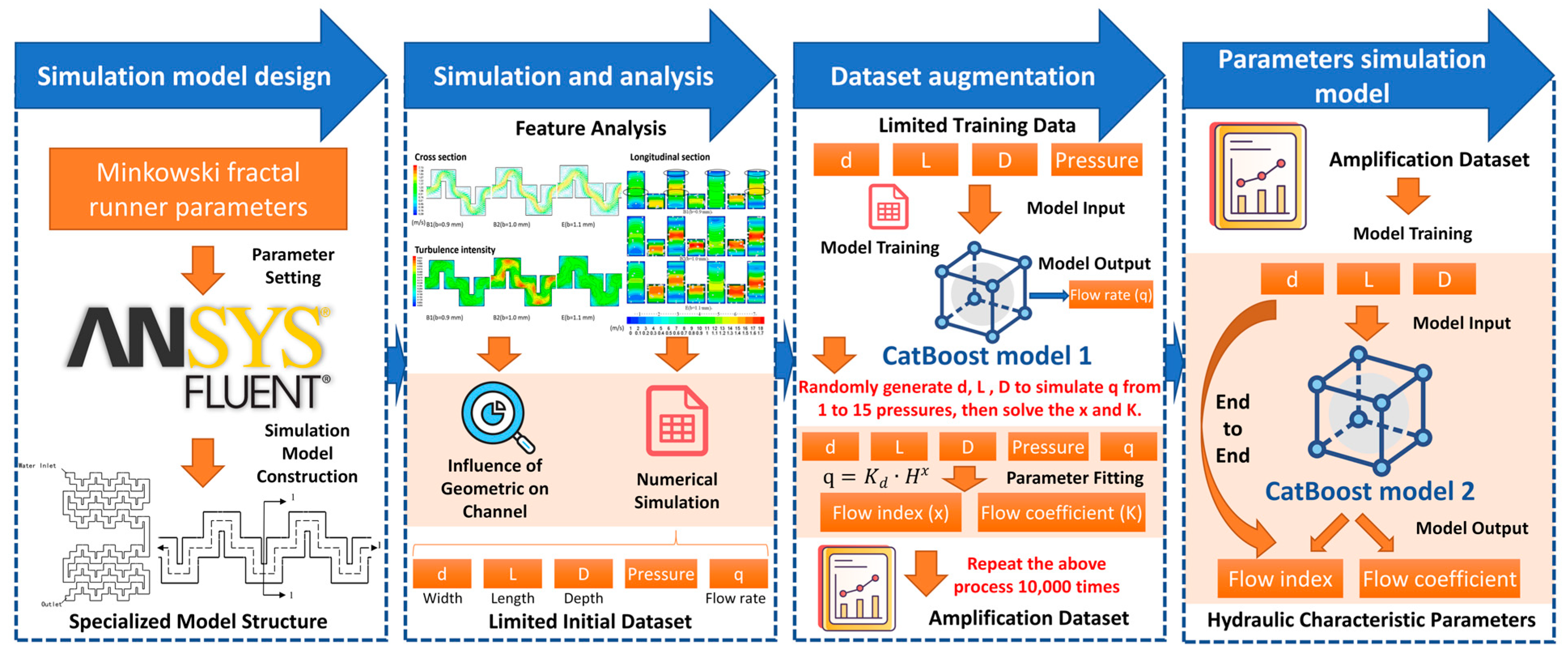
The framework of this study is shown in Figure 1, where the FLUENT software was used to simulate a model of a specific emitter type as a benchmark to simulate the flow rate at different pressures. Based on this, a small amount of simulation data were obtained to construct a fitting relationship between the four parameters of emitter depth, width, length and pressure, and flow rate to build a predictive model of emitter flow rate. Based on this model, the depth, width, and length parameters were randomly selected, as was the flow rate at 1–15 m pressure, and then the results of 15 simulations were used for regression analysis to derive the flow index and flow coefficient. The above process was repeated 10,000 times to form a data set of critical parameters of the emitter. Based on this, the model relationship between depth, width, and length as input conditions and flow index and flow was further implemented using the CatBoost model. Under the condition of a small amount of simulated real-world data, in order to maximize the use and reflect the actual accuracy, the model training in this study was used to evaluate the fitting accuracy by the leave-one-out cross-validation (LOOCV) method.

2.1. Method of Physical Simulation and Analysis of the Emitter

2.1.1. Numerical Methods

• Mathematical modeling

The standard k-ε turbulence model was used in this paper. The water flow in the emitter was considered as an unpressurized flow with negligible heat exchange, so only the continuity equation, the Navier-Stokes equation, and the turbulence equation were considered as the governing equations:

Continuous equations:

$$\frac{\partial \left(\mathrm{u}\right)}{\partial \mathrm{x}}+\frac{\partial \left(\mathrm{v}\right)}{\partial \mathrm{y}}+\frac{\partial \left(\mathrm{w}\right)}{\partial \mathrm{z}}=0$$

(1)

$$\frac{\partial \mathrm{u}}{\partial \mathrm{x}}+\frac{\partial \mathrm{v}}{\partial \mathrm{y}}+\frac{\partial \mathrm{w}}{\partial \mathrm{z}}=0$$

(2)

N-S equation:

$$\frac{\partial \left(\mathsf{\rho }\mathrm{u}\right)}{\partial \mathrm{t}}+\nabla ·\left(\mathsf{\rho }\mathrm{uu}\right)=\mathsf{\mu }{\nabla }^2\mathrm{u}-\frac{\partial \mathrm{p}}{\partial \mathrm{x}}+{\mathrm{S}}_{\mathrm{u}}$$

(3)

$$\frac{\partial \left(\mathsf{\rho }\mathrm{v}\right)}{\partial \mathrm{t}}+\nabla ·\left(\mathsf{\rho }\mathrm{vu}\right)=\mathsf{\mu }{\nabla }^2\mathrm{v}-\frac{\partial \mathrm{p}}{\partial \mathrm{y}}+{\mathrm{S}}_{\mathrm{v}}$$

(4)

$$\frac{\partial \left(\mathsf{\rho }\mathrm{w}\right)}{\partial \mathrm{t}}+\nabla ·\left(\mathsf{\rho }\mathrm{wu}\right)=\mathsf{\mu }{\nabla }^2\mathrm{w}-\frac{\partial \mathrm{p}}{\partial \mathrm{z}}+{\mathrm{S}}_{\mathrm{w}}$$

(5)

k-ε model:

$$\frac{\partial \left(\mathsf{\rho }\mathrm{k}\right)}{\partial \mathrm{t}}+\frac{\partial \left({\mathsf{\rho }\mathrm{ku}}_{\mathrm{i}}\right)}{\partial {\mathrm{x}}_{\mathrm{i}}}=\frac{\partial }{\partial {\mathrm{x}}_{\mathrm{j}}}\left[\left(\mathsf{\mu }+\frac{{\mathsf{\mu }}_{\mathrm{t}}}{{\mathsf{\sigma }}_{\mathrm{k}}}\right)\frac{\partial \mathrm{k}}{\partial {\mathrm{x}}_{\mathrm{j}}}\right]+{\mathrm{G}}_{\mathrm{k}}-\mathsf{\rho }\mathsf{\epsilon }$$

(6)

$$\frac{\partial \left(\mathsf{\rho }\mathsf{\epsilon }\right)}{\partial \mathrm{t}}+\frac{\partial \left({\mathsf{\rho }\mathsf{\epsilon }\mathrm{u}}_{\mathrm{i}}\right)}{\partial {\mathrm{x}}_{\mathrm{i}}}=\frac{\partial }{\partial {\mathrm{x}}_{\mathrm{j}}}\left[\left(\mathsf{\mu }+\frac{{\mathsf{\mu }}_{\mathrm{t}}}{{\mathsf{\sigma }}_{\mathsf{\epsilon }}}\right)\frac{\partial \mathsf{\epsilon }}{\partial {\mathrm{x}}_{\mathrm{j}}}\right]+\frac{{\mathrm{C}}_{1\mathsf{\epsilon }}}{\mathrm{k}}{\mathrm{G}}_{\mathrm{k}}-{\mathrm{C}}_{2\mathsf{\epsilon }}\mathsf{\rho }\frac{{\mathsf{\epsilon }}^2}{\mathrm{k}}$$

(7)

where $\mathrm{u}$ is the velocity vector, $\mathrm{u}$, $\mathrm{v},$ and $\mathrm{w}$ are velocity components, ${\mathrm{S}}_{\mathrm{u}},{ \mathrm{S}}_{\mathrm{v}}$ and ${\mathrm{S}}_{\mathrm{w}}$ are generalized source terms, ${\mathrm{u}}_{\mathrm{i}}$ is the time-averaged velocity, ${\mathsf{\mu }}_{\mathrm{t}}$ is the turbulent viscosity, $\mathrm{k}$ is the turbulent kinetic energy, $\mathsf{\epsilon }$ is the dissipation rate, ${\mathrm{G}}_{\mathrm{k}}$ is the turbulent energy generation term due to the mean velocity gradient, ${\mathrm{C}}_{1\mathsf{\epsilon }}$ = 1.44, ${\mathrm{C}}_{2\mathsf{\epsilon }}$ = 1.92, $\partial \mathrm{k}$ = 1.0, ${\mathsf{\sigma }}_{\mathsf{\epsilon }}$ = 1.3.

• Initial and Boundary Conditions

The inlet of the flow channel was set as the pressure inlet (in the range of 0.01–0.15 MPa). The value was taken as the working pressure at each 0.01 MPa interval. There were 15 horizontal inlets. The pressure output was atmospheric pressure. The wall boundary was a non-slip boundary, taking into account the influence of the viscous subsurface, using standard wall function processing.

• Model solving

The finite volume method was used to discrete the control equations. The discrete format was based on discrete convection terms in first-order windward format and discrete diffusion terms in central difference format. The steady-state calculation, solved by the separate SIMPLE algorithm, was calculated with a convergence accuracy of 0.0001.

2.1.2. Physical Model Design of the Emitter

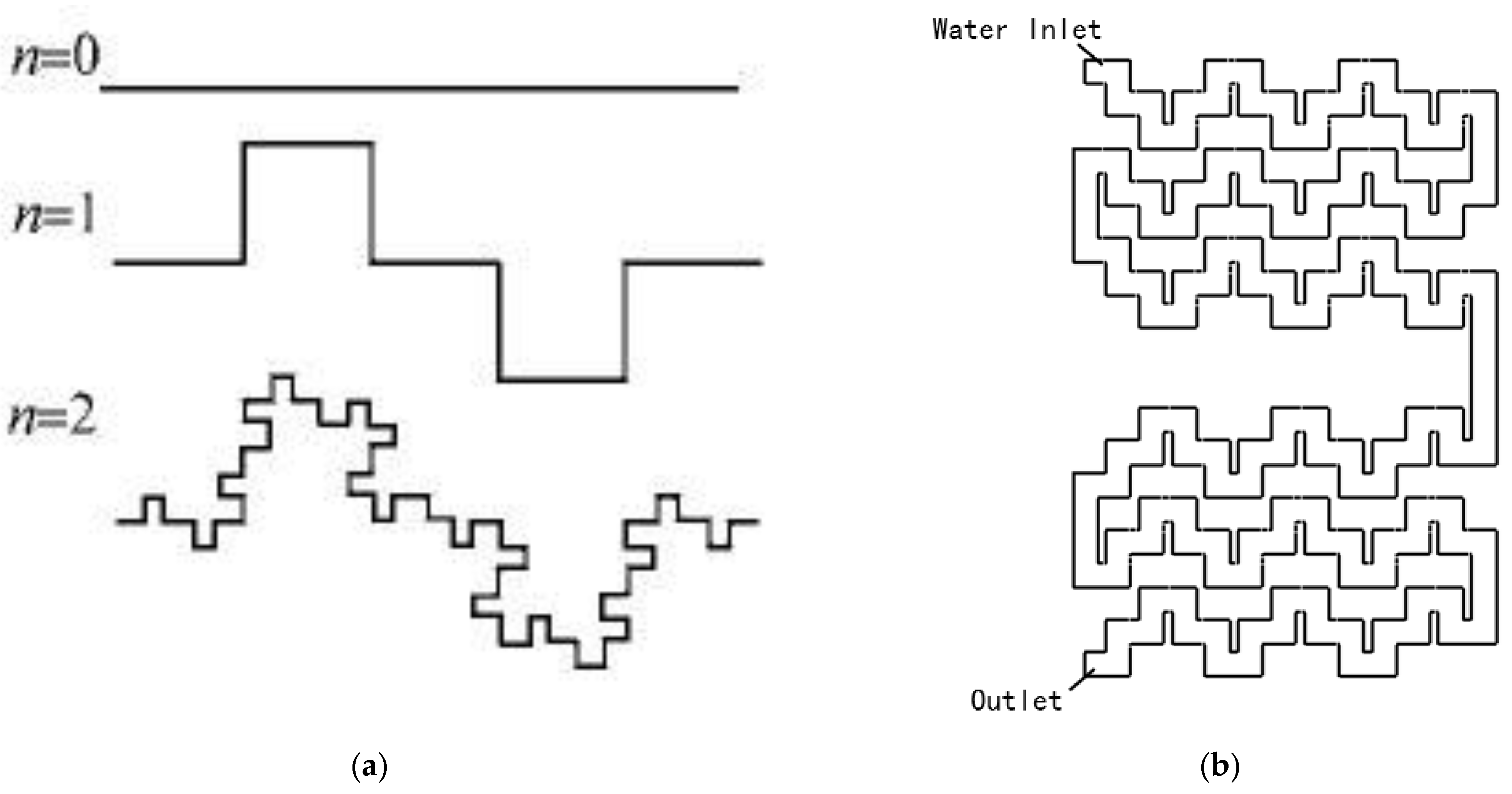
The design of the emitter flow path mainly uses the Minkowski fractal flow path; the basic square steps are as follows: (1) as in Figure 2 (n = 0), a straight line of length Lm is selected; (2) as in Figure 2 (n = 1), the straight line segment is divided into five equal parts and retains the first, third and fifth segments are retained, the second and fourth segments are changed to the angle of 90° in turn perpendicular to the three long Lm/5 straight line segments selected path width; (3) as in Figure 2 (n = 2), the five straight line segments of length Lm/5 are divided into five equal parts, and the first, third, and fifth line segments in each group of five equal parts are retained, and the second and fourth line segments are changed to three straight line segments of length Lm/25 at an angle of 90°. The Minkowski fractal curve generated by n = 2 iterations is used as the boundary. The distance b is extended to the other side and modified, keeping the geometric parameters of the flow path energy dissipation unit unchanged. The Minkowski fractal flow path is formed, as shown in Figure 2b.

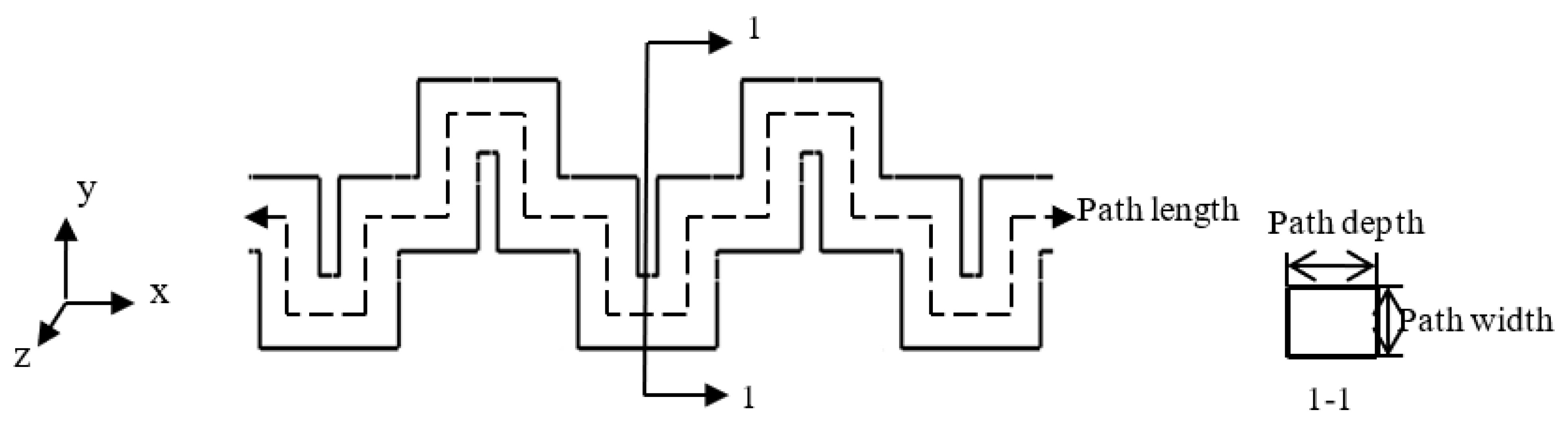
Based on their generation process and fractal characteristics (Figure 3), the generated path energy dissipation units have the same structural parameters, such as path tooth height and rotation angle, when a certain Euclidean length Lm is determined. Therefore, only three independent factors of path width (b), path depth (D), and path length (L) need to be selected as the structural geometry parameters for path design to control the structural dimensions of the path. The Minkowski fractal flow path with 13 different structural parameters was designed and constructed, and the geometric modeling was conducted in the Pro/E platform.

2.1.3. Model Validation

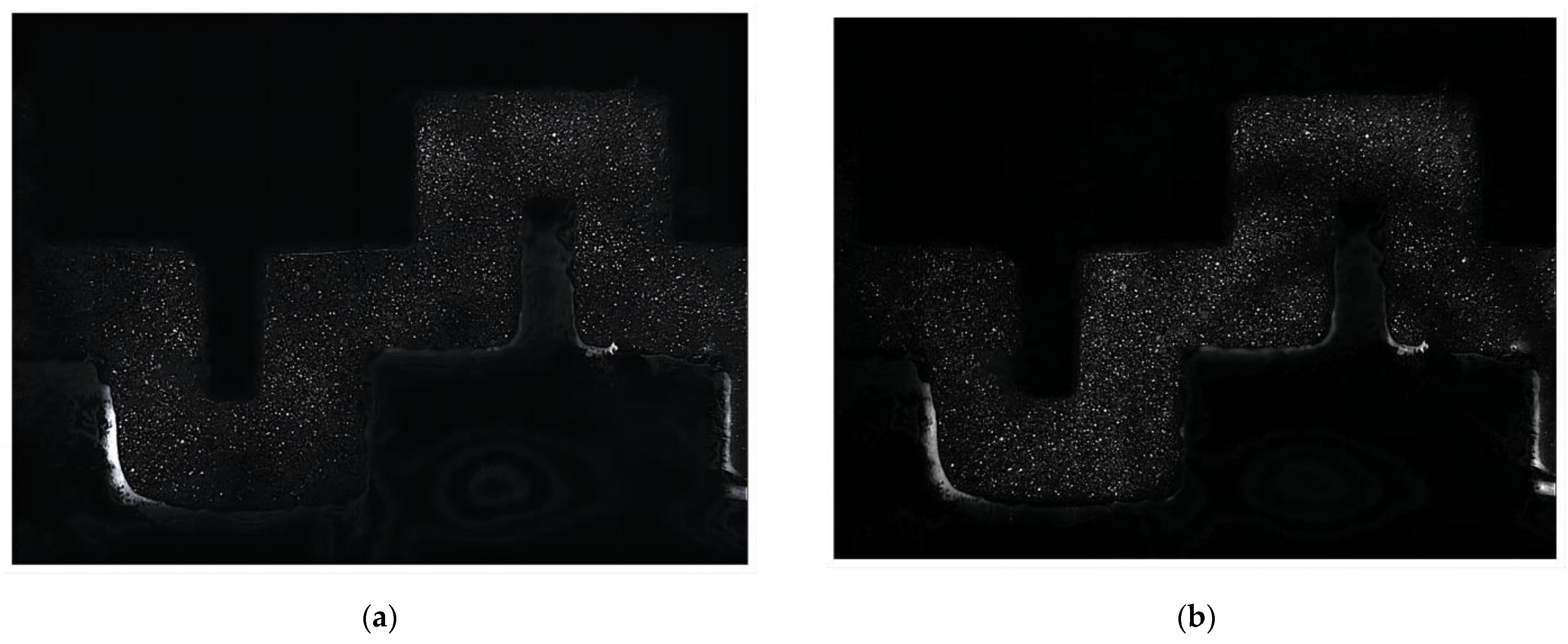
Digital Particle Image Velocimetry (DPIV) is a method of digitizing traditional image velocimetry PIV technology. The leading equipment of the Digital Particle Image Velocimetry system, the image acquisition equipment is the Kodak MEGA PLUS II camera (resolution 1600 × 1200, 2 M). The camera lens is an objective microscope lens (specification: 4×, model G10-211) manufactured by Beijing Daheng Camera Factory; the laser light source system is a Q-modulated Nd: YAG double-pulse laser manufactured by LABEST. The fluorescent particles were selected for testing. The primary material was polystyrene, the density was about 1020 kg/m³, and the concentration was 1–2%. The image acquisition, display, and computational analysis software are TSI insight3G, and the set interval time is 0.01 s. Taking flow path B3 as an example, Figure 4 shows the particle distribution images in the flow path structure unit at the adjacent moments before and after. Image post-processing was performed using the Tecplot software included with insight 3.

2.1.4. Numerical Design of Experiments

According to the characteristics of the fractal flow path, it is known that the width, depth, and length of the flow path are the key parameters. Therefore, three basic parameters were selected for the study in the following ranges: path width within [0.9 mm, 1.3 mm], path depth within [0.9 mm, 1.3 mm], and path length within [128 mm, 256 mm]. Five levels of each parameter were selected, with one set of duplicates, resulting in 13 different structural geometry parameters for the paths (

Table 1. Experimental design parameters for different structural geometry parameters of the Minkowski fractal flow path.

Path Type	Path Width (b, mm)	Path Depth (D, mm)	Path Length (L, mm)
B1	0.9	1.1	192
B2	1	1.1	192
B3	1.2	1.1	192
B4	1.3	1.1	192
D1	1.1	0.9	192
D2	1.1	1.0	192
D3	1.1	1.2	192
D4	1.1	1.3	192
L1	1.1	1.1	128
L2	1.1	1.1	160
L3	1.1	1.1	224
L4	1.1	1.1	256
E	1.1	1.1	192

).

2.1.5. Analysis Method

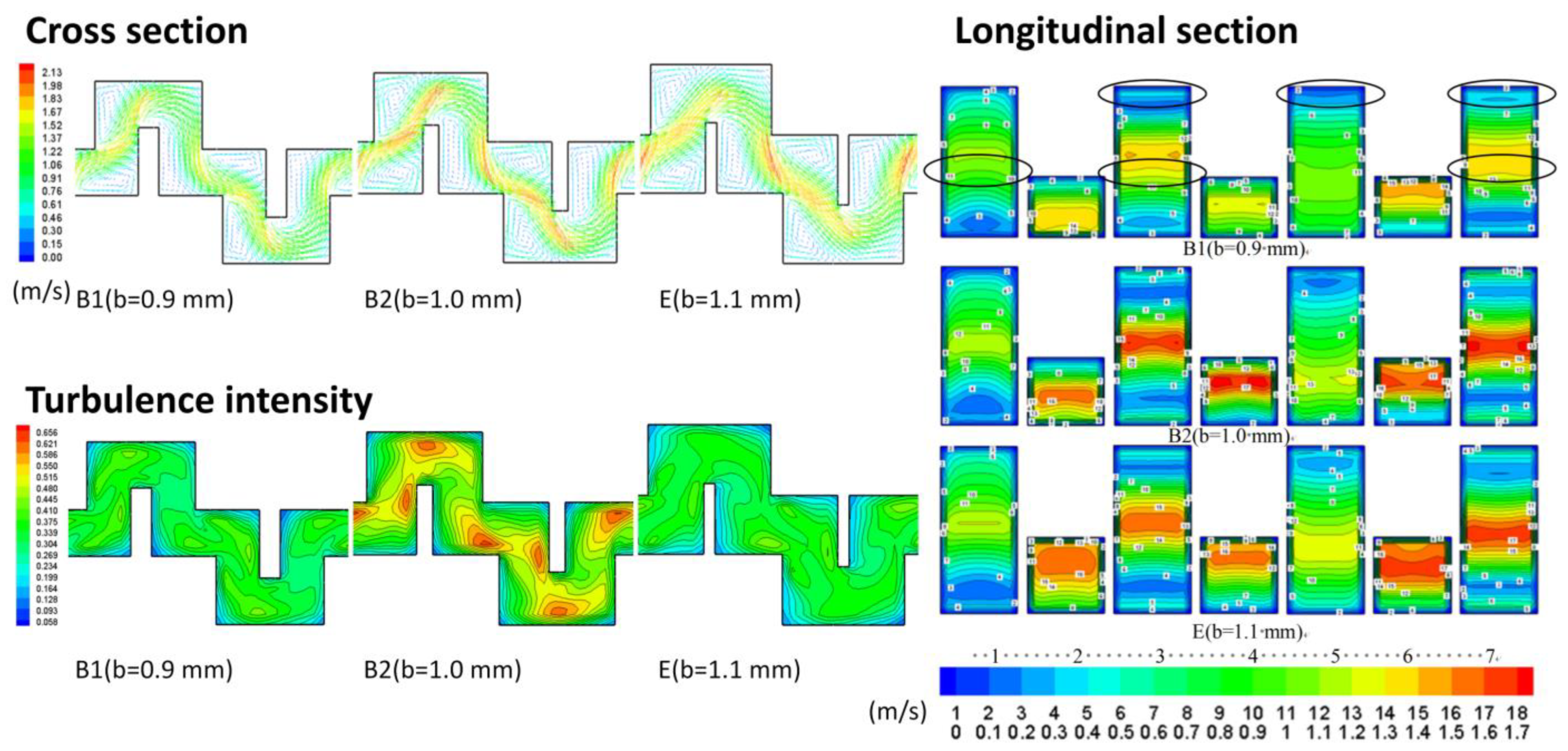
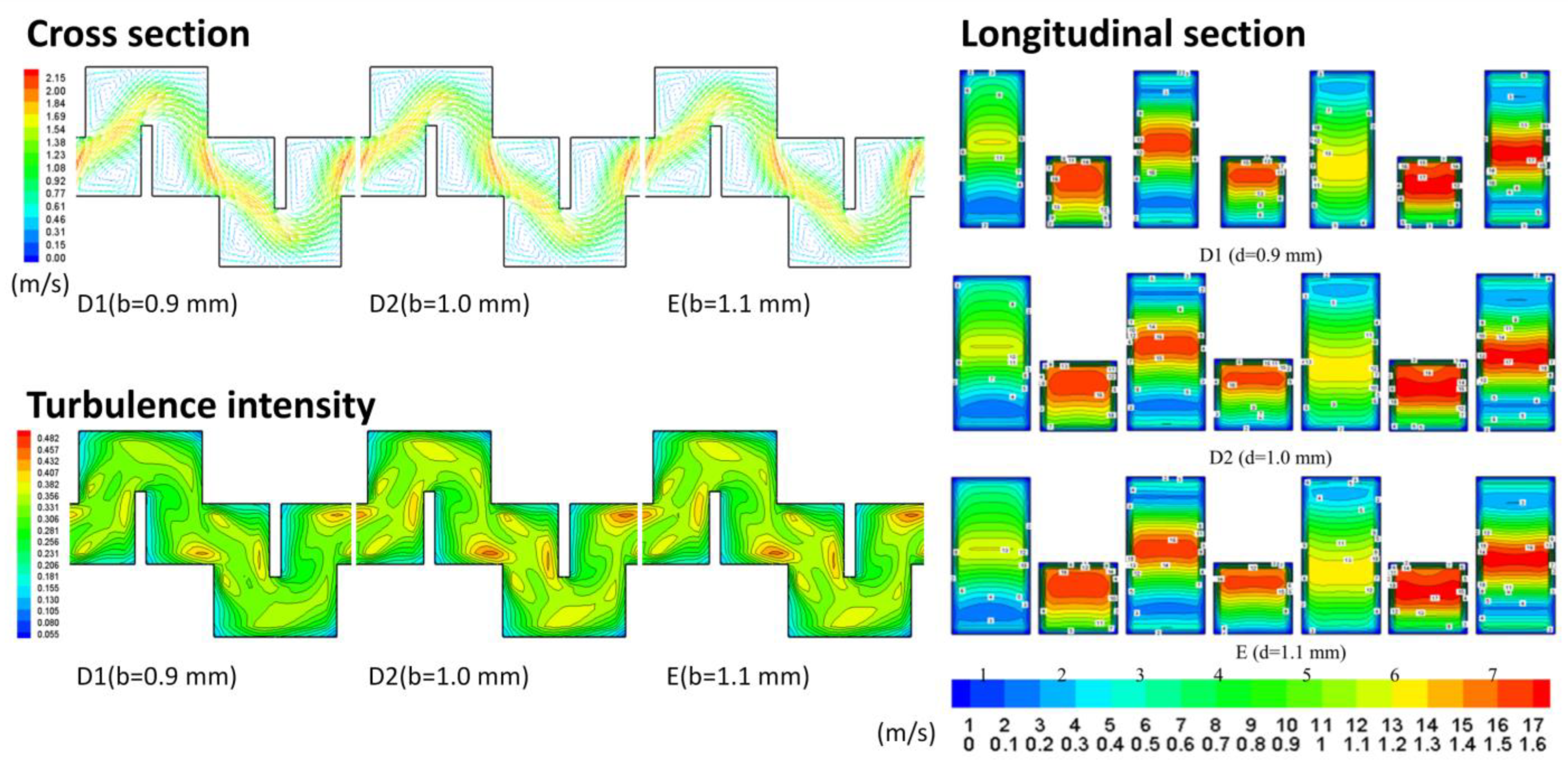
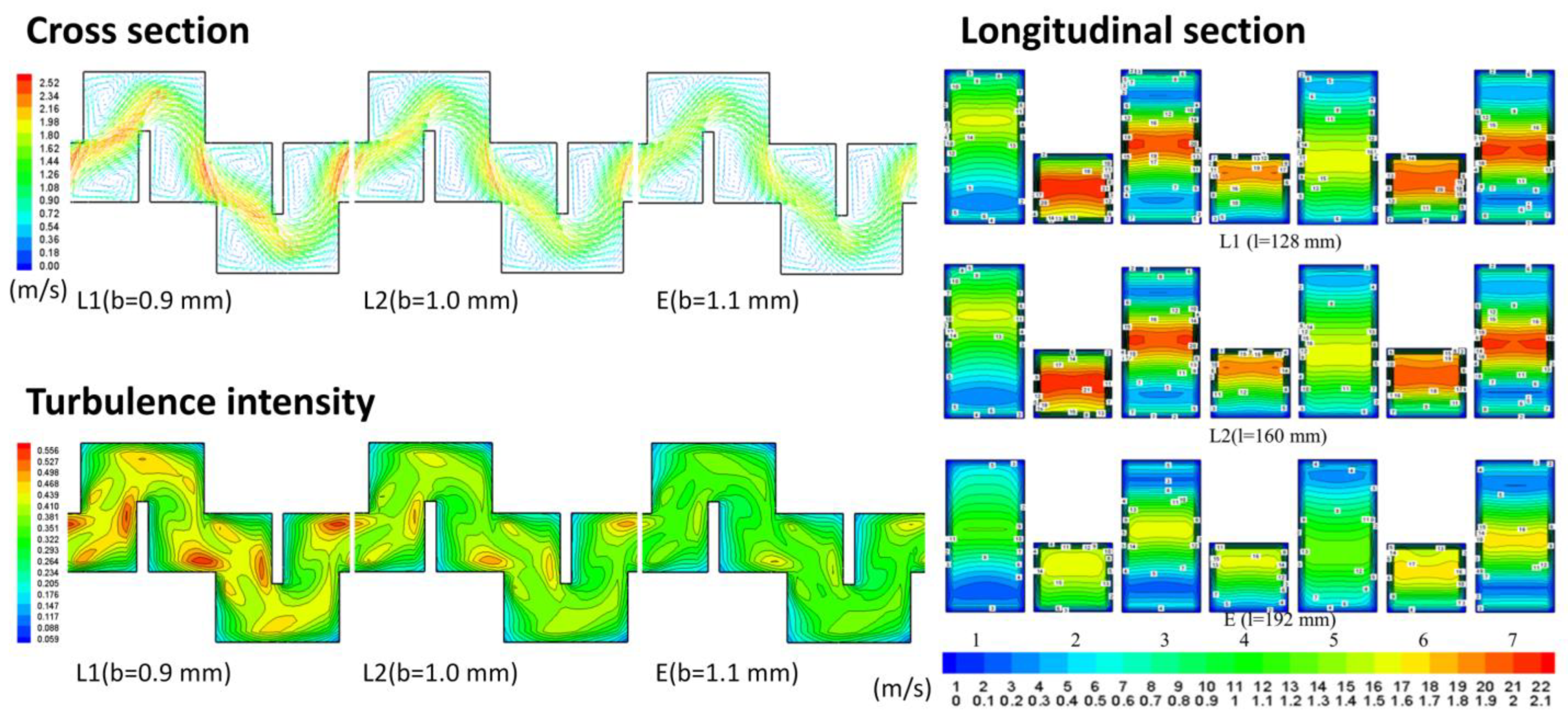
Numerical simulations are performed using FLUENT 6.3 for the constructed fractal flow channels with different structural parameters. By visualizing the microscopic internal flow field, the variation of the flow field and hydraulic properties can be studied. It facilitates the analysis of the flow characteristics and mechanism of the internal flow field. Three groups of representative flow channels (B1, B2, E), (D1, D2, E), and (L1, L2, E) are selected for different flow channel widths, depths, and lengths to visualize the distribution of internal flow characteristic parameters at an operating pressure of 0.1 MPa.

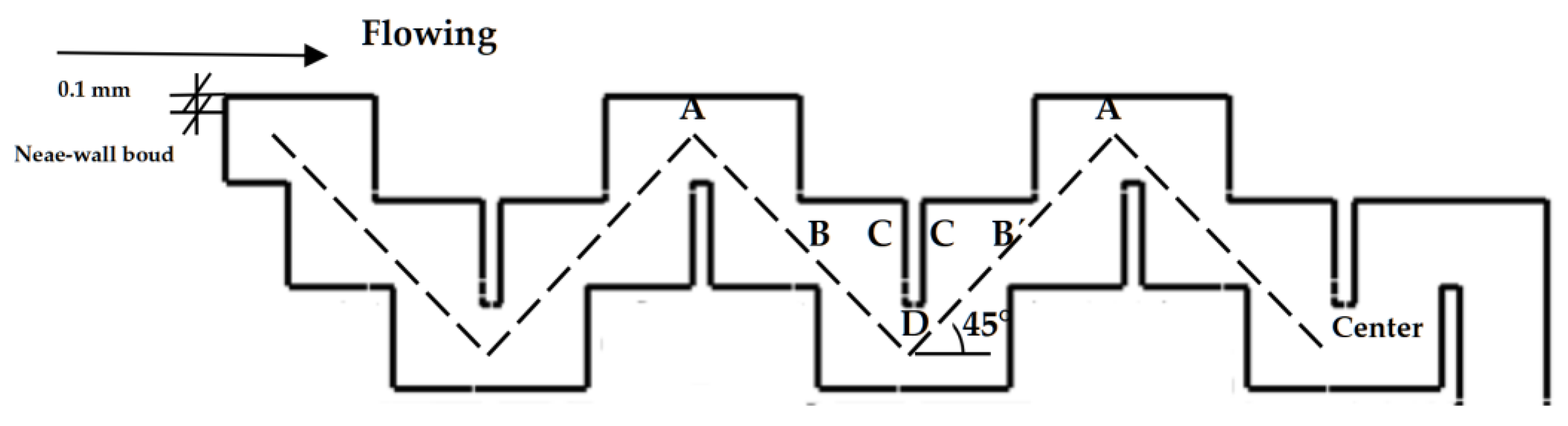
• Cross-sectional velocity distribution

As in Figure 5, the fractal flow path section (Z = 0.5D) is taken, and the near wall surface is set at 0.1 mm from the top wall as the structural change along the boundary. The centerline of the flow path is selected from the midpoint of the inlet width of the flow path unit section, as shown in the schematic diagram. The Minkowski fractal flow path has several energy dissipation units with the same structure, so the analysis was refined to the flow path structural units. The velocity vector distribution of the cross-sectional (Z = 0.5D) flow path structural unit is visualized, and its velocity mass motion characteristics are analyzed.

• Longitudinal profile flow velocity distribution

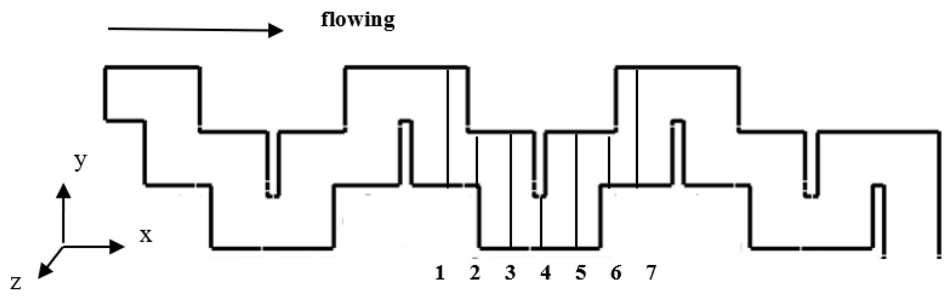
Seven longitudinal sections in the Y-Z plane were taken equidistantly at different locations along the forward direction of the water flow in the flow path unit section, as shown in Figure 6. The velocity contours of the seven longitudinal sections are observed to analyze the velocity distribution characteristics in the longitudinal sections.

• Turbulence intensity distribution map

Turbulence intensity reflects the intensity of flow pulsation. It is an important index to describe the turbulent motion characteristics of water flow, which can be used to measure the strength of the flow field. Therefore, turbulence intensity is also used as an analysis index in this paper when analyzing the flow motion characteristics within the flow path. The isotropic distribution of the turbulence intensity within the flow path structure unit is analyzed.

• Hydraulics performance analysis

According to the design, 13 fractal flow paths were simulated to calculate the fractal flow path discharge at 0.01 MPa operating pressure in the 0.01–0.15 MPa range. The following equation is used to describe the hydraulic performance of the flow path, the calculated flow value, and the operating pressure using regression calculations to obtain the flow index $\mathrm{x}$ and flow coefficient ${\mathrm{K}}_{\mathrm{d}}$ of different fractal flow paths at different operating levels.

$$\mathrm{q}={\mathrm{K}}_{\mathrm{d}}·{\mathrm{H}}^{\mathrm{x}}$$

(8)

where $\mathrm{q}$ is the flow rate, $\mathrm{H}$ is the working pressure, ${\mathrm{K}}_{\mathrm{d}}$ is the flow coefficient, and $\mathrm{x}$ is the exponent flow.

2.2. CatBoost Model

CatBoost is a gradient-boosting decision tree-based machine learning framework that implements extensions and improvements to the Gradient Boosting Decision Tree (GBDT) algorithm [24]. Unlike the traditional GBDT, the category feature processing process first randomly sorts all samples. Then, for a given value taken in the category-based features, each part of that feature to numerical is averaged based on the category label ranked before that sample, adding weighting factors for priority and precedence. This practice reduces the noise caused by low-frequency features in the category features. In the regression problem, the stress calculation is generally obtained by averaging the label values. Let a permutation be $\mathsf{\sigma }$ = (1, 2, …, n), then ${\mathrm{x}}_{{\mathsf{\sigma }}_{\mathrm{p},\mathrm{k}}}$ can be replaced by:

$${\mathrm{x}}_{{\mathsf{\sigma }}_{\mathrm{p},\mathrm{k}}}=\frac{{{\displaystyle \sum }}_{\mathrm{j}=1}^{\mathrm{p}-1}\left[{\mathrm{x}}_{{\mathsf{\sigma }}_{\mathrm{j},\mathrm{k}}}={\mathrm{x}}_{{\mathsf{\sigma }}_{\mathrm{p},\mathrm{k}}}\right]{\mathrm{Y}}_{{\mathsf{\sigma }}_{\mathrm{j}}}+\mathrm{a}\ast \mathrm{p}}{{{\displaystyle \sum }}_{\mathrm{j}=1}^{\mathrm{p}-1}\left[{\mathrm{x}}_{{\mathsf{\sigma }}_{\mathrm{j},\mathrm{k}}}={\mathrm{x}}_{{\mathsf{\sigma }}_{\mathrm{p},\mathrm{k}}}\right]+\mathrm{a}}$$

(9)

where, $\mathrm{a}$ is the weight coefficient greater than 0, and $\mathrm{p}$ is the added last term.

CatBoost obtains new features by combining category-based elements to improve prediction performance. When constructing a new tree, CatBoost uses a greedy approach to consider combinations to build the choice of split points. No variety is considered when the tree is split for the first time. At the next split, it combines all combinations of the current tree and category-based features with all category-based features in the dataset. It dynamically converts the new varieties of category-based features into numerical parts. Its pseudo code process is shown in Algorithm 1—Pseudocode for the tree construction method of the Catboost model.

Algorithm 1: Building a tree in CatBoost

Input: $\mathrm{M},{\left\{\left({\mathrm{X}}_{\mathrm{i}},{\mathrm{y}}_{\mathrm{i}}\right)\right\}}_{\mathrm{i}=1}^{\mathrm{n}},\mathsf{\alpha },\mathrm{L},{\left\{{\mathsf{\sigma }}_{\mathrm{i}}\right\}}_{\mathrm{i}=1}^{\mathrm{s}}, \mathrm{Mode}$

$\mathrm{grad} \leftarrow \mathrm{CalcGradient} \left(\mathrm{L}, \mathrm{M},\mathrm{y}\right)$

$\mathrm{r}\leftarrow \mathrm{random} \left(1,\mathrm{s}\right)$

$\mathbf{if} \mathrm{Mode}=\mathrm{Plain} \mathbf{then}$

$\mathrm{G}\leftarrow \left({\mathrm{grad}}_{\mathrm{r}}\left(\mathrm{i}\right) \mathrm{for} \mathrm{i} =1\dots \mathrm{n}\right)$

$\mathbf{if} \mathrm{Mode}=\mathrm{Ordered} \mathbf{then}$

$\mathrm{G}\leftarrow \left({\mathrm{grad}}_{\mathrm{r},{\mathsf{\sigma }}_{\mathrm{r}}\left(\mathrm{i}\right)-1}\left(\mathrm{i}\right) \mathrm{for} \mathrm{i}=1\dots \mathrm{n}\right)$

$\mathbf{T}\leftarrow \mathrm{empty} \mathrm{tree};$

$\mathbf{foreach} \mathrm{step} \mathrm{of} \mathrm{top}-\mathrm{down} \mathrm{procedure} \mathbf{do}$

$\mathbf{foreach} \mathrm{candidate} \mathrm{split} \mathrm{c} \mathbf{do}$

${\mathrm{T}}_{\mathrm{c}}\leftarrow \mathrm{add} \mathrm{split} \mathrm{c} \mathrm{to} \mathrm{T}$

$\mathbf{if} \mathrm{Mode}=\mathrm{Plain} \mathbf{then}$

$\mathsf{\Delta }\left(\mathrm{i}\right)\leftarrow \mathrm{avg}\left({\mathrm{grad}}_{\mathrm{r}}\left(\mathrm{p}\right){ \mathrm{forp}:\mathrm{leaf} }_{\mathrm{r}}\left(\mathrm{p}\right)={\mathrm{leaf}}_{\mathrm{r}}\left(\mathrm{i}\right)\right) \mathrm{for} \mathrm{i}=1\dots \mathrm{n}$

$\mathbf{if} \mathrm{Mode}=\mathrm{Ordered} \mathbf{then}$

$\mathsf{\Delta }\left(\mathrm{i}\right)\leftarrow \mathrm{avg}\left({\mathrm{grad}}_{\mathrm{r},{\mathsf{\sigma }}_{\mathrm{r}}\left(\mathrm{i}\right)-1}\left(\mathrm{p}\right){ \mathrm{forp}:\mathrm{leaf}}_{\mathrm{r}}\left(\mathrm{p}\right)={\mathrm{leaf}}_{\mathrm{r}}\left(\mathrm{i}\right),{\mathsf{\sigma }}_{\mathrm{r}}\left(\mathrm{p}\right)<{\mathsf{\sigma }}_{\mathrm{r}}\left(\mathrm{i}\right)\right)$

$\mathrm{for} \mathrm{i}=1\dots \mathrm{n}$

In addition, CatBoost replaces the gradient estimation method in the traditional algorithm with ordered boosting, which reduces the bias of the gradient estimation and improves the generalization ability of the model. To obtain unbiased gradient estimation, CatBoost trains a separate model ${\mathrm{M}}_{\mathrm{i}}$ for each sample ${\mathrm{X}}_{\mathrm{i}}$, the model ${\mathrm{M}}_{\mathrm{i}}$ is obtained by using a training set that does not contain samples ${\mathrm{X}}_{\mathrm{i}}$. The gradient estimate over the sample is obtained using ${\mathrm{M}}_{\mathrm{i}}$. The gradient is used to train the base learner and obtain the final model. The pseudo-code of the ordered boosting algorithm is shown in Algorithm 2—Ordered boosting algorithm.

Algorithm 2: Ordered boosting

Input: ${\left\{\left({\mathrm{X}}_{\mathrm{k}},{\mathrm{y}}_{\mathrm{k}}\right)\right\}}_{\mathrm{k}=1}^{\mathrm{n}},\mathrm{I};$

$\mathsf{\sigma }\leftarrow \mathrm{random} \mathrm{permutation} \mathrm{of} \left[1, \mathrm{n}\right];$  ${\mathrm{M}}_{\mathrm{i}}\leftarrow 0 \mathrm{for} \mathrm{i}=1\dots \mathrm{n}$

$\mathbf{for} \mathrm{t}\leftarrow 1 \mathbf{to} \mathrm{I} \mathbf{do}$

$\mathbf{for} \mathrm{i}\leftarrow 1 \mathbf{to} \mathrm{n} \mathbf{do}$

${\mathrm{r}}_{\mathrm{i}}\leftarrow {\mathrm{y}}_{\mathrm{i}} - {\mathrm{M}}_{\mathsf{\sigma }\left(\mathrm{i}\right)-1}\left({\mathrm{X}}_{\mathrm{i}}\right)$

$\mathbf{for} \mathrm{i}\leftarrow 1 \mathbf{to} \mathrm{n} \mathbf{do}$

$\mathsf{\Delta }\mathrm{M}\leftarrow$  $\mathrm{Learn} \mathrm{Model} \left(\left({\mathrm{X}}_{\mathrm{j}},{\mathrm{r}}_{\mathrm{j}}\right):\mathsf{\sigma }\left(\mathrm{j}\right)\le \mathrm{i}\right)$

${\mathrm{M}}_{\mathrm{i}}\leftarrow {\mathrm{M}}_{\mathrm{i}}+\mathsf{\Delta }\mathrm{M}$

${\mathbf{return} \mathrm{M}}_{\mathrm{n}}$

In this study, the default hyperparameter values (

Table 2. Information on the main parameters of the CatBoost model.

Parameters	Type	Default Value	Explanations
iterations	int	1000	The maximum number of trees can be built when solving machine learning problems.
learning rate	float	0.03	The learning rate. It is used for reducing the gradient step.
depth	int	6	Depth of the tree. The range of supported values depends on the processing unit type and the type of the selected loss function.
l2_leaf_reg	float	3	Coefficient at the L2 regularization term of the cost function. Any positive value is allowed.
loss_function	string	MSE	Loss function
border_count	int	128	The number of splits for numerical features. Allowed values are integers from 1 to 65,535 inclusively. Recommended values are up to 255. Larger values slow down the training.
ctr_border	int	1	The number of category feature separators.

) were used for the parameter configuration of CatBoost to facilitate model evaluation and subsequent application.

2.3. Cross-Validation and Evaluation Criteria

K-fold cross-validation is an essential method in machine learning. The data set is randomly divided into k copies, with the training set taking k-1 copies and the test set taking one copy. Each data set is used as a training set, and the remaining k-1 data sets are used as training sets. Thus, a total of K iterations are required for each round of training. Considering the small amount of data simulated by CFD simulation, this study uses leave-one-out cross-validation (LOOCV) to evaluate the generalization fit accuracy of the model [25]. LOOCV is a unique form of k-fold cross-validation, which can be considered as n-fold cross-validation when k is equal to the sample size n. This means that one datum at a time is taken out as the only element of the test set. All remaining (n-1) data points are the corresponding training set, and n iterations are required for each round of training. The model hyperparameters and generalization ability are evaluated by calculating the average error over all iterations (Figure 7). The advantage of LOOCV is that each data set is treated individually as a test set, so it is not affected by the training of the test set. The advantage of LOOCV is that each datum is individually conducted as a test set. It is not affected by the test set training set partitioning method, can make full use of the data, prevent model overfitting from occurring, and assess the actual generalization ability of the model. The combined error $\mathrm{LOOCV}\left(\mathrm{n}\right)$ can be expressed as:

$$\mathrm{LOOCV}\left(\mathrm{n}\right)=\frac{1}{\mathrm{n}}{{\displaystyle \sum }}_{\mathrm{i}=1}^{\mathrm{n}}{\mathrm{MSE}}_{\mathrm{i}}$$

(10)

Four evaluation measures were selected to indicate the performance of the CatBoost model.

The mean absolute error (MAE):

$$\mathrm{MAE}=\frac{1}{\mathrm{m}}{{\displaystyle \sum }}_{\mathrm{i}=1}^{\mathrm{m}}\left|\left({\mathrm{y}}_{\mathrm{i}}-\stackrel{\wedge }{{\mathrm{y}}_{\mathrm{i}}}\right)\right|$$

(11)

The mean squared error (MSE):

$$\mathrm{MSE}=\frac{1}{\mathrm{m}}{\displaystyle \sum }_{\mathrm{i}=1}^{\mathrm{m}}{\left({\mathrm{y}}_{\mathrm{i}}-\stackrel{\wedge }{{\mathrm{y}}_{\mathrm{i}}}\right)}^2$$

(12)

The root mean squared error (RMSE):

$$\mathrm{RMSE}=\sqrt{\frac{1}{\mathrm{m}}{\displaystyle \sum }_{\mathrm{i}=1}^{\mathrm{m}}{\left({\mathrm{y}}_{\mathrm{i}}-\stackrel{\wedge }{{\mathrm{y}}_{\mathrm{i}}}\right)}^2}$$

(13)

The mean absolute percentage error (MAPE):

$$\mathrm{MAPE}=\frac{100}{\mathrm{n}}{\displaystyle \sum }_{\mathrm{i}=1}^{\mathrm{n}}\left|\frac{\stackrel{\wedge }{{\mathrm{y}}_{\mathrm{i}}}-{\mathrm{y}}_{\mathrm{i}}}{\stackrel{\wedge }{{\mathrm{y}}_{\mathrm{i}}}}\right|$$

(14)

The coefficient of determination (R²):

$${\mathrm{R}}^2=1-\frac{{{\displaystyle \sum }}_{\mathrm{i}}{\left(\stackrel{\wedge }{{\mathrm{y}}_{\mathrm{i}}}-{\mathrm{y}}_{\mathrm{i}}\right)}^2}{{{\displaystyle \sum }}_{\mathrm{i}}{\left(\overline{{\mathrm{y}}_{\mathrm{i}}}-{\mathrm{y}}^{\mathrm{i}}\right)}^2}$$

(15)

In the above formulas, $\stackrel{\wedge }{{\mathrm{y}}_{\mathrm{i}}}$ is the predicted value, ${\mathrm{y}}_{\mathrm{i}}$ is the true value, and $\overline{{\mathrm{y}}_{\mathrm{i}}}$ is the average value. MAE can reflect the actual situation of the predicted value error. MSE is the expected value of the square of the difference between the estimated and the observed value; it can evaluate the degree of the data change, and the smaller the MSE, the better accuracy of the prediction model. RMSE is the arithmetic square root of MSE. MAPE is equivalent to normalizing the error at each point, reducing the impact of the absolute error from individual outliers. R² can eliminate the influence of dimension on the evaluation measure.

2.4. Model Training

The training environment for the experiments in this study is a graphics workstation configured with a CPU: Intel(R) Core(TM) i9-10980XE CPU @ 3.00 GHz, GPU: NVIDIA GeForce RTX 3090, and RAM: 64 GB. Model training uses the Anaconda platform as the model training base, Spyder as the integrated development tool, CatBoost version 0.25.1 as the model framework, and the underlying Python version 3.7. Considering that CatBoost models can conveniently mobilize GPU arithmetic for computation, and the configuration of the experimental environment can further enhance the efficiency of model training.

2.5. CFD Simulation Results

The FLUENT software was used for the numerical simulation, and the k-ε model was selected to solve the flow field using the SIMPLE algorithm. The flow path inlet is set as a pressure inlet, and the value is taken as the drop inlet pressure every 1 m in the range of 1–15 m, with a total of 15 horizontal inputs. The outlet of the flow path is set to atmospheric pressure, and the wall is treated with the wall function. The simulated flow values were obtained, as shown in

Table 3. Simulated flow values in the fractal flow path at different working pressures.

Path Type	Flow Rate (m/s)
Pressure (m)	1	2	3	4	5	6	7	8	9	10	11	12	13	14	15
B1	0.939	1.328	1.619	1.862	2.076	2.268	2.445	2.608	2.762	2.908	3.043	3.173	3.297	3.415	3.529
B2	0.986	1.376	1.671	1.918	2.135	2.338	2.534	2.692	2.862	3.016	3.152	3.289	3.421	3.548	3.670
B3	1.386	1.947	2.368	2.725	3.038	3.320	3.578	3.817	4.041	4.251	4.450	4.641	4.825	5.004	5.171
B4	1.537	2.167	2.645	3.046	3.397	3.714	4.007	4.274	4.525	4.763	4.990	5.203	5.408	5.606	5.796
D1	0.993	1.410	1.724	1.990	2.223	2.435	2.625	2.805	2.974	3.131	3.279	3.422	3.560	3.691	3.816
D2	1.223	1.730	2.116	2.441	2.726	2.982	3.217	3.436	3.640	3.832	4.015	4.187	4.353	4.514	4.665
D3	1.338	1.892	2.311	2.664	2.976	3.255	3.514	3.753	3.976	4.185	4.383	4.571	4.755	4.928	5.096
D4	1.452	2.051	2.507	2.890	3.226	3.530	3.808	4.066	4.307	4.532	4.752	4.953	5.149	5.338	5.522
L1	1.475	2.082	2.543	2.932	3.273	3.578	3.857	4.115	4.358	4.586	4.805	5.013	5.215	5.403	5.591
L2	1.320	1.866	2.282	2.630	2.939	3.213	3.466	3.698	3.920	4.123	4.324	4.510	4.683	4.861	5.023
L3	1.056	1.484	1.809	2.072	2.316	2.524	2.739	2.945	3.091	3.275	3.441	3.593	3.710	3.869	3.994
L4	1.048	1.486	1.817	2.096	2.339	2.561	2.765	2.950	3.129	3.292	3.551	3.598	3.743	3.879	4.009
E	1.212	1.714	2.097	2.418	2.700	2.952	3.186	3.402	3.606	3.793	3.973	4.147	4.309	4.468	4.617

.

3. Results

3.1. Influence of Different Geometric Parameters on the Flow Characteristics of the Flow Field in the Flow Path

(1) For the effect of flow characteristics of the flow field in the flow path of different widths (b) (Figure 8). The overall flow characteristics of the flow field in the cross-section are the velocity in the flow path varies periodically, the high-speed mass drives the low-speed liquid mass, the low-speed liquid mass stalls the high-speed liquid mass flow, and mixes to show the characteristics of turbulent flow. The flow field in the longitudinal direction of the flow characteristics: The velocity distribution varies more in the vertical direction of the flow channel width. The velocity variation along the channel depth x direction is small. A secondary flow phenomenon appears within the flow field distribution. As the flow path width increases, the velocity of the central zone and the vortex zone in the flow path develop sufficiently, but the increase from B2 to E flow path is not significant. The overall distribution of turbulence intensity is characterized as follows: the turbulence intensity reaches its maximum at the corners of the flow path and out between the teeth. The turbulence intensity in the vortex zone is over 10%, which belongs to the high turbulence zone. The high pulsation of the turbulent flow can slow down particle deposition, while the shear force generated by the vortex has a destructive effect on particle agglomeration.

(2) For the effect of the flow characteristics of the flow field in the flow path at different depths (D) (Figure 9). The maximum flow velocities of flow paths D1, D2, and E are 2.15 m/s, 2.13 m/s, and 2.13 m/s, respectively. The flow velocity at the outer edge of the vortex region is within [0.30 m/s, 0.46 m/s] for VD1, [0.30 m/s, 0.46 m/s] for VD2, [0.30 m/s, 0.45 m/s] for VE. From the longitudinal section, the changes in the size of the velocity distribution in the main flow area and near the wall are insignificant as the flow path depth increases. 1, 3, 5, and 7 wide flow path cross-sectional prominent flow area locations are located in the middle of the cross-section. 2, 4, and 6 narrow flow path central flow area locations are located in the upper part of the flow path cross-section, and their locations are not shifted with the change of flow path depth. In general, the flow field structure within the fractal flow path is similar in depth direction. With the evolution of the flow path depth, the flow velocity, turbulence intensity distribution, and size do not differ much. The flow characteristics are very similar in the depth direction.

(3) For the effect of different path lengths (L) on the flow path characteristics (Figure 10). The velocity decreases linearly as the flow path length increases, and the maximum flow velocities in flow paths L1, L2, and E are 2.52 m/s, 2.28 m/s, and 2.13 m/s, respectively. The velocities at the outer edge of the vortex zone are within [0.49 m/s, 0.66 m/s], [0.40 m/s, 0.53 m/s], and [0.30 m/s, 0.45 m/s]. From the longitudinal cross-sectional velocity field, the velocity in the main flow area and near the wall shows a significant decreasing trend with increasing path depth, which is consistent with the cross-sectional variation law. The change in flow path depth does not shift the position of the main flow region. Based on this in the flow path design, the flow path length can be changed to adjust the hydraulic performance of the emitter. The turbulence intensity distribution structure is similar for different flow path lengths, and the turbulence intensity decreases as the flow path length increases. L1, L2, and E flow paths turbulence intensity in flow path turbulence intensity was in the range of [6.5%, 55.6%], [6.1%, 52.5%], and [5.9%, 48.2%], respectively.

3.2. Correlation between Different Structural Geometric Parameters and Macroscopic Hydrodynamic Properties

Figure 11 shows the variation of flow index and flow coefficient (at the 0.05 level) under the influence of different parameters in the extended data set, calculated using the Pearson correlation coefficient method. The values of d, D, and L are taken in the ranges of [0.9 mm, 1.3 mm], [0.9 mm, 1.3 mm], and [128 mm, 256 mm], respectively. The extended data set is obtained from the uniformity of the data distribution by fitting the flow prediction model and coefficient. The uniformity of b, D, and L shows that the extended data set can effectively cover the specified range. From the correlation of the hydraulic characteristic parameters, the flow coefficient has the highest correlation coefficient with b (r = 0.6114). While the flow index has the highest negative correlation relationship with L (r = −0.2534), and the flow index and the flow coefficient show some negative correlation relationship with each other (r = −0.2943).

3.3. Accuracy of Flow Simulation with Small Amount of Simulation Data

Figure 12 shows the accuracy of the emitter flux prediction model based on a small number of simulated data sets. Each point in the figure shows the relationship between the true and predicted values for a moment in the leave-one-out cross-validation that was not included in the model training. The overall prediction accuracy of the model is high, with average MAE, MSE, RMSE, MAPE, and R² of 0.0261, 0.0025, 0.0498, and 0.9987, respectively. The flow prediction model trained by CatBoost can accurately perform flow prediction for different emitter parameters and pressures.

Figure 13 shows the importance scores of the input variables of the emitter flow prediction model, demonstrating the degree of importance of the different input variables in influencing the prediction accuracy of the model. The average importance scores of the four input variables are ranked as follows: pressure (46.20) > b (27.28) > L (16.74) > D (9.78). Overall, the change in pressure has the most significant effect on the prediction of the model flow. The distribution of important scores for each indicator over the training period is quite consistent. The 25–75% importance scores of pressures, b, L, and D were within [40.96, 50.72], [23.39, 32.66], [12.36, 22.23] and [7.72, 12.27], respectively.

3.4. Prediction Accuracy of Flow Index and Flow Coefficient under Extended Dataset Conditions

Figure 14 shows the accuracy of the prediction model for the emitter flow index based on the extended dataset. The figure contains a total of 10,000 iterations of cross-validation of the actual versus predicted values of the flow index for each of the omitted test points. The cross-validation results show that the model can predict the flow index with high accuracy, with average MAE, MSE, RMSE, MAPE, and R² of 0.0021, 0.00002, 0.0047, and 0.9961, respectively. The CatBoost model can accurately predict the corresponding flow index at pressures of 1–15 m by inputting three parameters (d, D, and L).

Figure 15 shows the importance scores of the input variables for the model prediction of the emitter flow index. The average importance scores of the three input indicators are ordered as b (55.97) > L (25.71) > D (18.32). Overall, the change in b has the most significant effect on the prediction of the model flow index, and the importance score distribution of each indicator over training is significantly clustered. The 25–75% importance scores of b, L, and D are in the range of [55.07, 56.75], [25.15, 26.33], and [17.96, 18.69], respectively.

Figure 16 shows the accuracy of the prediction model for the emitter flow coefficient based on the extended data set. The figure also shows the relationship between the actual and predicted values. The flow coefficient for each of the 10,000 iterations of cross-validation on the full dataset, excluding the test points. The cross-validation results show that the model can also predict the flow coefficient with high accuracy, with average MAE, MSE, RMSE, MAPE, and R² of 0.0261, 0.00026, 0.0161, and 0.9946, respectively. The CatBoost model can accurately predict the corresponding flow coefficient at 1–15 m pressure by inputting three parameters (d, D, and L).

Figure 17 illustrates the importance scores of the input variables for the emitter flow coefficient prediction model. In contrast to the trend of the importance scores for the flow index, the average importance scores for the three input variables are in the following order: b (45.20) > D (27.98) > L (26.82). The overall change in b has the most significant effect on the prediction of the model flow coefficient, and the distribution of importance scores for each indicator is significantly clustered. The importance of D exceeds that of L in predicting the flow coefficient. Variables b, D, and L have importance scores in the range of 25–75% within [44.33, 46.05], [27.13, 28.82], and [26.15, 27.50], respectively.

3.5. Comparison of Prediction Accuracy of Different Models for Flow Rate, Flow Index and Flow Coefficient

In order to evaluate the prediction accuracy of the proposed models, some classical machine learning models similar to CatBoost were selected for comparison, namely XGBoost [26], Bagging [27], Random Forest [28], Tree [29], Adaboost [30] and KNN [31]. Different models were trained using the simulated and extended datasets, respectively, and the accuracy of the model predictions was also evaluated using LOOCV.

Table 4. Comparison of the accuracy of different models for predicting flow rate, flow index, and flow coefficient.

Algorithm	Flow Rate				Flow Index				Flow Coefficient
	MSE	MAE	RMSE	R2	MSE	MAE	RMSE	R2	MSE	MAE	RMSE	R2
CatBoost	0.0025	0.0261	0.0498	0.9987	0.00002	0.0021	0.0047	0.9961	0.0003	0.0261	0.0161	0.9946
XGBoost	0.0274	0.1171	0.1655	0.9864	0.00005	0.0043	0.0072	0.9909	0.0007	0.0141	0.0258	0.9891
Bagging	0.0439	0.1174	0.2097	0.9783	0.0005	0.0044	0.0074	0.9903	0.0006	0.0143	0.0243	0.9877
Random Forest	0.0675	0.1867	0.2598	0.9667	0.00008	0.0053	0.0092	0.9851	0.0008	0.0143	0.0277	0.9841
Tree	0.1317	0.2862	0.3629	0.9351	0.0002	0.0052	0.0123	0.9729	0.0012	0.0105	0.0339	0.9763
Adaboost	0.1835	0.3476	0.4284	0.9094	0.0005	0.0184	0.0224	0.9105	0.0096	0.0836	0.0982	0.8011
KNN	0.4489	0.5047	0.6701	0.7784	0.0034	0.0461	0.0583	0.3162	0.0351	0.1465	0.1876	0.2769

compares the accuracy of the different models in predicting flow rate, flow index, and flow coefficient. Overall, the CatBoost model used in this study has the best accuracy in predicting different indices. The prediction accuracy of the other models is ranked as follows: CatBoost > XGBoost > Bagging > Random Forest > Tree > Adaboost > KNN, while XGBoost, which is also an ensemble learning model with CatBoost, also achieves good prediction accuracy, while KNN has difficulty in achieving good prediction results for different metrics.

4. Discussion

As one of the most efficient irrigation technologies, drip irrigation technology can achieve more than 90% water-saving efficiency and has been widely used worldwide [17]. The small size of the emitter path, generally around 0.5–1.2 mm, and the variation of its path geometry directly affect the hydraulic performance of the emitter, which has a significant impact on its anti-clogging performance, irrigation uniformity, and service life [6]. Current research on the relationship between flow path structural parameters and hydraulic properties has received some attention [15,16]. However, the real reason for the change in hydraulic properties is that the change in flow path structural parameters affects the characteristic flow parameters of the internal flow field. Studies on the relationship between the flow path structural parameters, internal flow characteristics, and hydraulic characteristics of emitters are rare.

There have been studies on hydraulic performance, mainly using the flow index and flow coefficient as evaluation indices. Among the findings on the effect of structural parameters on the flow index, many studies have shown that flow path geometry parameters have a more pronounced effect on the flow index. Ref. [32] studied the relationship between hydraulic performance and flow path length of inlaid sheet emitters and concluded that as the flow path length increases, there is a correlation with the flow index. Ref. [33] performed an ANOVA on triangular loop flow paths and found that the flow path width had a significant effect on the flow index. 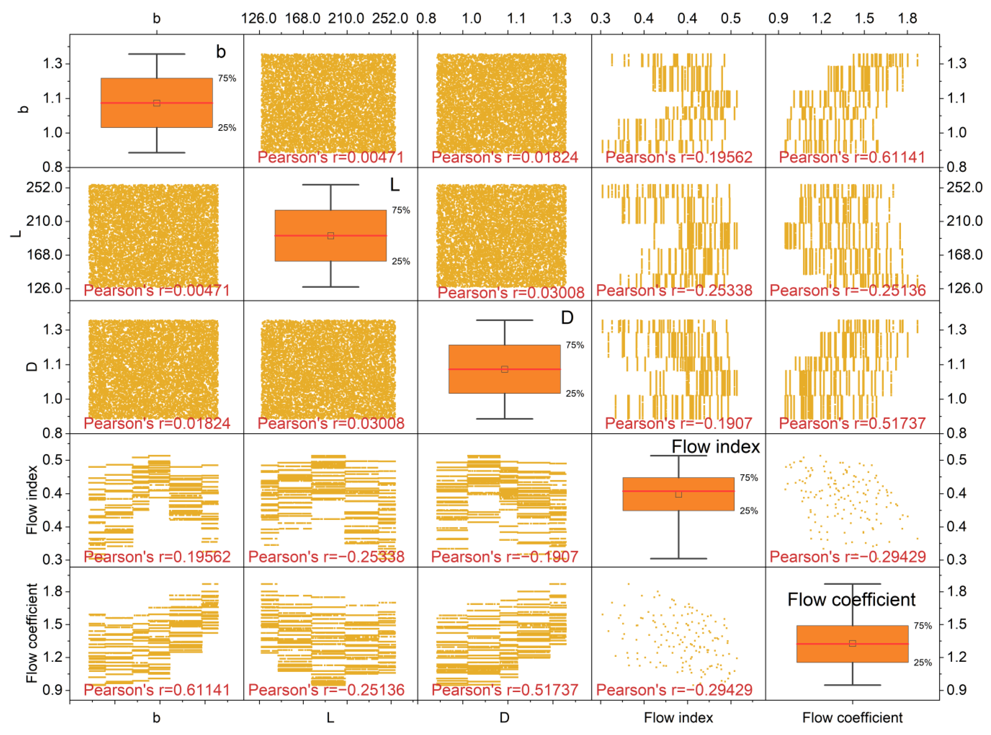In [34], the flow path width, twist angle, height, upper bottom width, and offset were selected as key flow path parameters to perform ANOVA and extreme difference analysis on the hydraulic performance of the toothed labyrinth flow path. It was found that the top-bottom width and turning angle had a significant effect on the flow index. 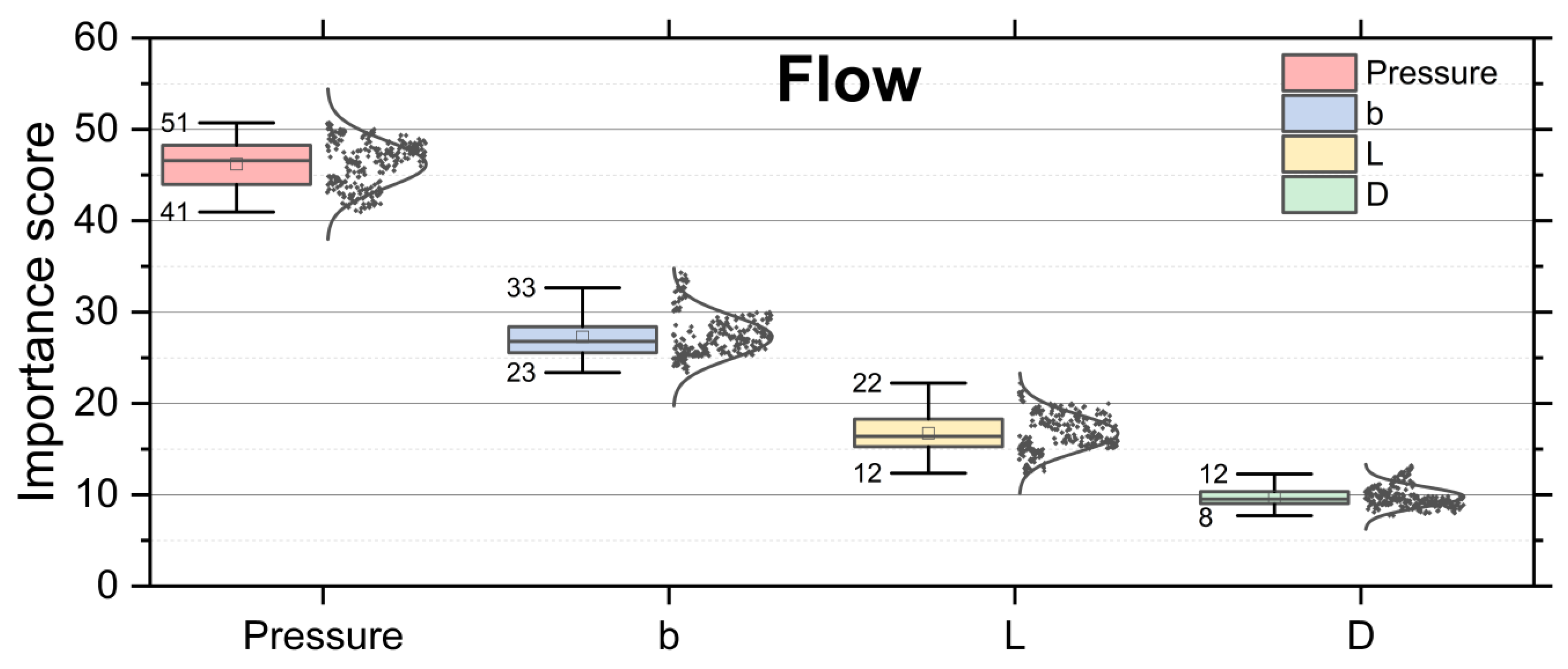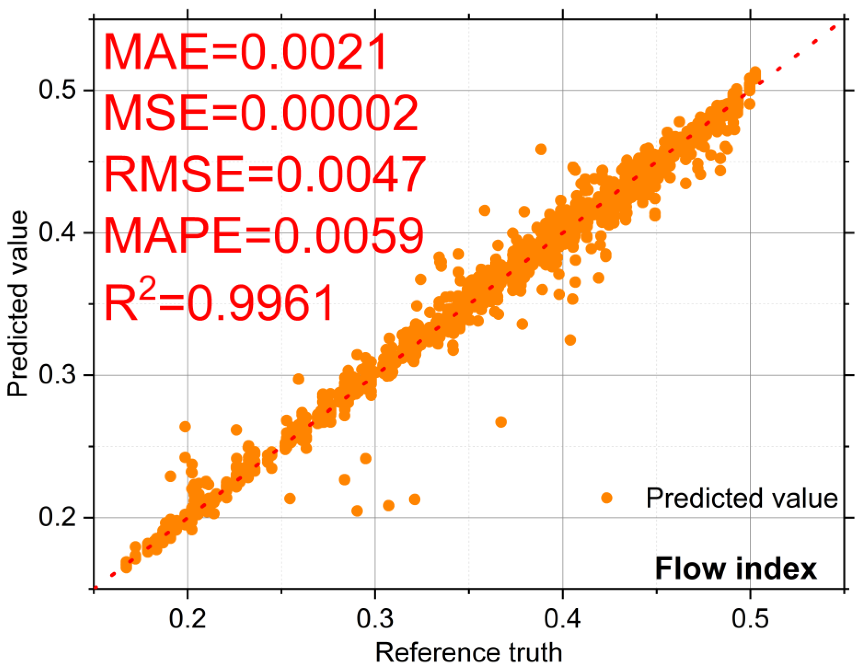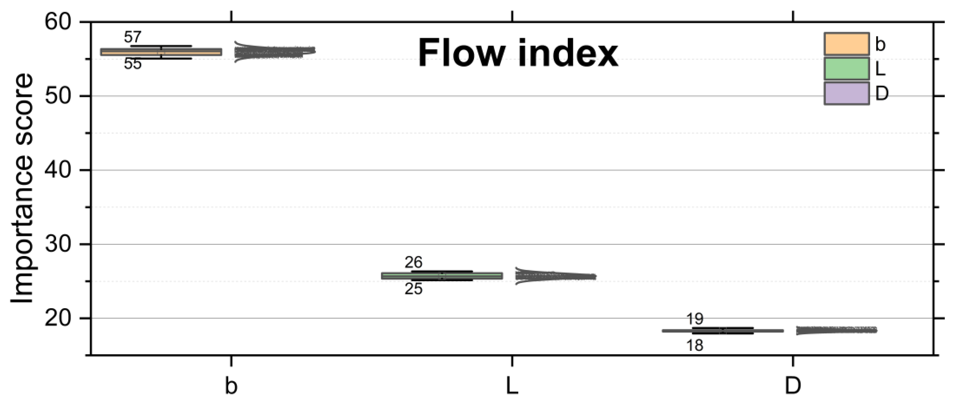This is consistent with the results shown in Figure 11 of this study. Among them, the correlation coefficient between the flow index and b reaches 0.6114, which has a significant positive correlation. The correlation coefficient with L also reaches −0.2514, with a more obvious negative correlation characteristic. In addition, the average model importance score of the b parameter on the flow index is 55.97, which significantly affects the predictive effect of the flow index (Figure 15).

As a scale factor characterizing the emitter scale, the flow coefficient has a dominant effect on the flow rate and is proportional to the flow rate. Studies on the relationship between flow path geometry and flow coefficient variation have all concluded that flow path structural parameters significantly affect the flow coefficient, which is consistent with the results of this study (Figure 11). In the case of the inlay patch flow path, [32] concluded that the flow coefficient decreases as the length of the flow path increases. Ref. [33] concluded that the height of the flow path unit, the inlet size, the height of the flow path, and the depth all have a significant effect on the flow coefficient of the triangular return flow path. Ref. [34] concluded that the depth, width, inlet size, and unit height of the labyrinth flow path all significantly affect the flow coefficient. Ref. [13] concluded that the flow path geometry significantly affects the flow coefficient of the patch emitter. The flow coefficient varies significantly as the cross-sectional area increases and decreases as the number of cells increases. 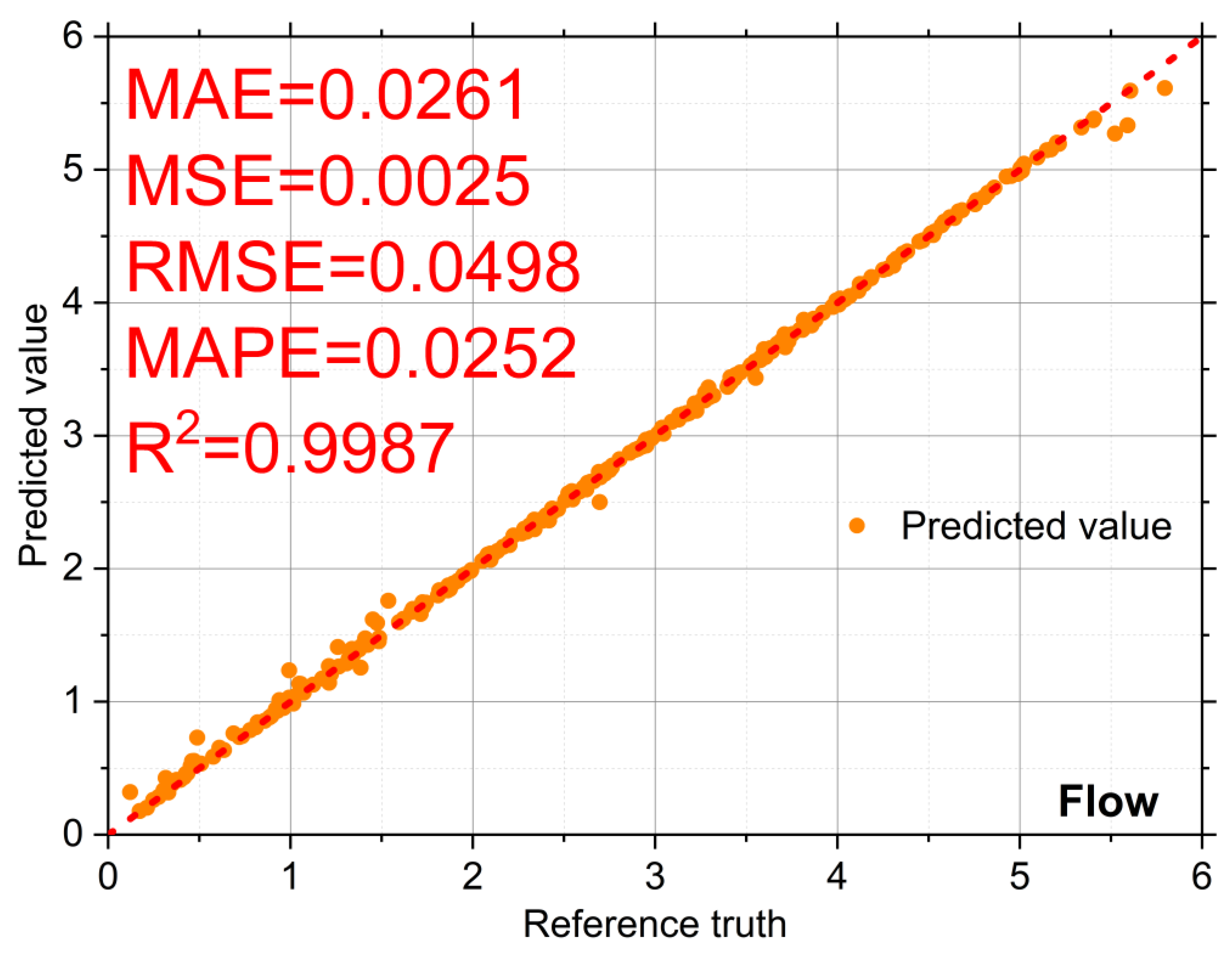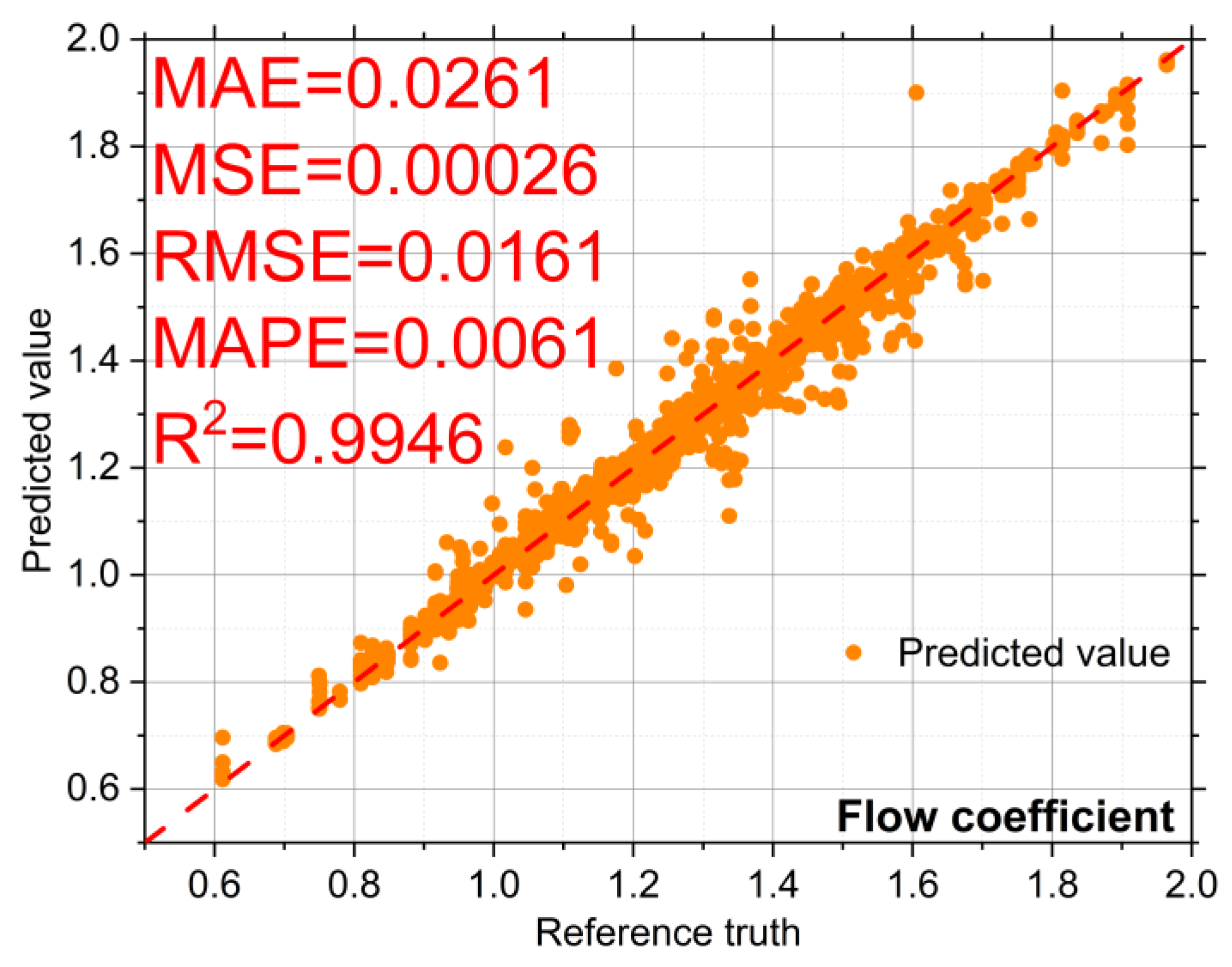This study also shows that the flow coefficient is strongly influenced by the geometric parameters of the flow path structure and that the width, depth, and length of the flow path are positively correlated with the flow coefficient (Figure 17). 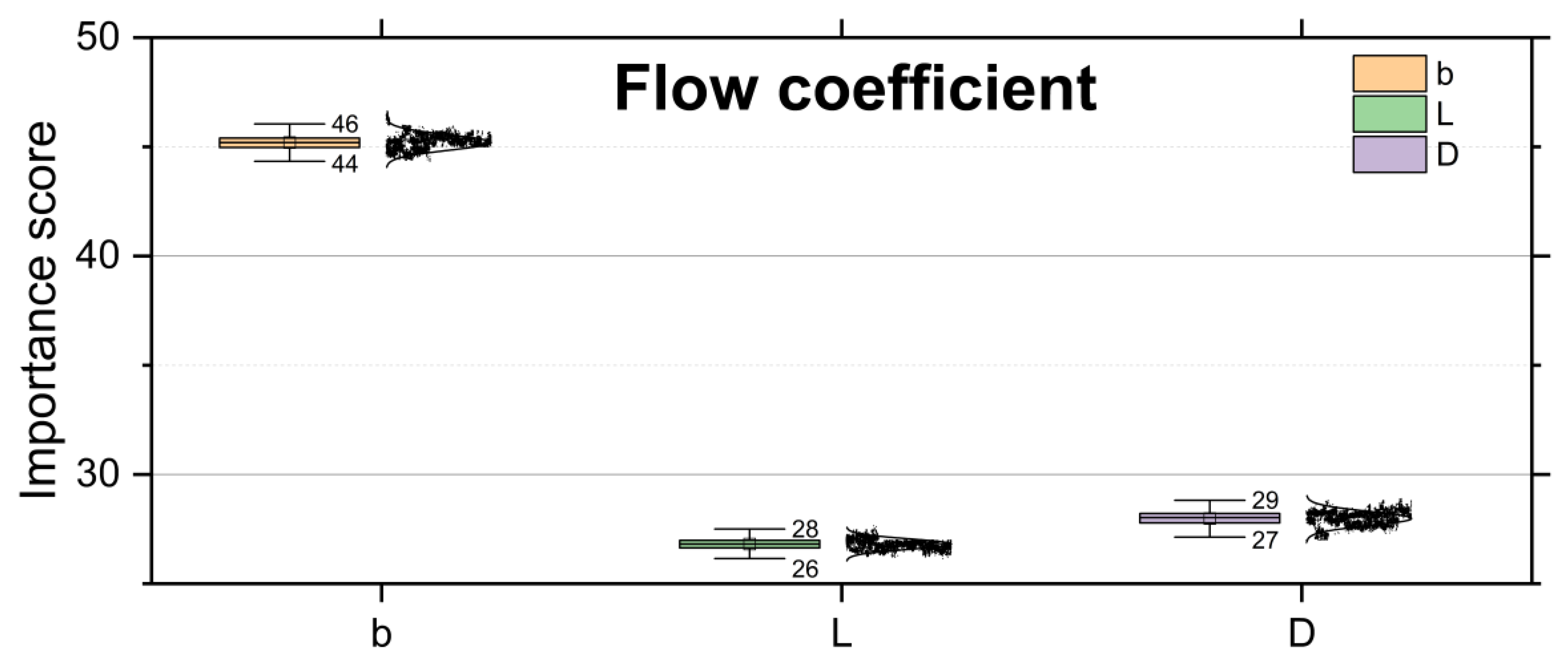Based on this, the MAE of the prediction model of the flow coefficient by the geometric parameters of the flow path structure is only 0.0261 (Figure 16) and has a high correlation (R² = 0.9946). In addition, b also had the highest importance score (45.2) for the flow coefficient prediction model, showing a strong influence on the flow coefficient (Figure 17).

The CatBoost model showed an excellent fit with a prediction accuracy R² greater than 0.99 for flow rate, flow index, and flow coefficient. As for the differences in prediction accuracy between the different algorithms, the ensemble learning algorithm was able to extract better features and fit trends by integrating the results of many weak learners. The result is similar to other studies using the CatBoost model [28]. In addition, the resulting XGBoost model has a lower prediction accuracy than the CatBoost model with default parameters, and the studies of [22,23,34] also confirm the advantages of the CatBoost model.

5. Conclusions

In this study, a small number of morphological parameters were simulated using FLUENT software to analyze the influence of flow rate. The CatBoost model was used to construct a flow rate prediction model based on the simulation. The results of this study show that the significant correlation between the geometric structure and the flow index and flow coefficient provides the basis for the correlation model. CatBoost can fit the complex nonlinear relationships between the parameters well, achieving excellent simulation accuracy for flow rate (R² = 0.9987), flow index (R² = 0.9961), and flow coefficient (R² = 0.9946), where b has the highest importance score in the model construction for the flow regime index (score = 55.97) and flow coefficient (score = 45.2). Furthermore, the CatBoost models used in this study achieved the best prediction results compared to their typical counterparts (XGBoost, Bagging, Random Forest, Tree, Adaboost, and KNN). This study can provide more reliable and efficient technical support for agricultural production, which can help improve agricultural production efficiency and reduce water waste.

References

1. Cole, M.B.; Augustin, M.A.; Robertson, M.J.; Manners, J.M. The Science of Food Security. NPJ Sci. Food 2018, 2, 14. [Google Scholar] [CrossRef] [PubMed]
2. Owusu, P.A.; Asumadu-Sarkodie, S.; Ameyo, P. A review of Ghana’s water resource management and the future prospect. Cogent Eng. 2016, 3, 1164275. [Google Scholar] [CrossRef]
3. Vörösmarty, C.J.; McIntyre, P.B.; Gessner, M.O.; Dudgeon, D.; Prusevich, A.; Green, P.; Glidden, S.; Bunn, S.E.; Sullivan, C.A.; Liermann, C.R.; et al. Global threats to human water security and river biodiversity. Nature 2010, 467, 555–561. [Google Scholar] [CrossRef] [PubMed] [Green Version]
4. Liao, R.; Zhang, S.; Zhang, X.; Wang, M.; Wu, H.; Zhangzhong, L. Development of smart irrigation systems based on real-time soil moisture data in a greenhouse: Proof of concept. Agric. Water Manag. 2020, 245, 106632. [Google Scholar] [CrossRef]
5. Si, Z.; Zain, M.; Mehmood, F.; Wang, G.; Gao, Y.; Duan, A. Effects of nitrogen application rate and irrigation regime on growth, yield, and water-nitrogen use efficiency of drip-irrigated winter wheat in the North China Plain. Agric. Water Manag. 2020, 231, 106002. [Google Scholar] [CrossRef]
6. Irmak, S.; Brar, D.; Kukal, M.S.; Odhiambo, L.; Djaman, K. Automated real-time irrigation analytics inform diversity in regional irrigator behavior and water withdrawal and use characteristics. Agric. Water Manag. 2022, 272, 107837. [Google Scholar] [CrossRef]
7. van der Kooij, S.; Zwarteveen, M.; Boesveld, H.; Kuper, M. The efficiency of drip irrigation unpacked. Agric. Water Manag. 2013, 123, 103–110. [Google Scholar] [CrossRef]
8. Ren, Z.; Lv, B.; Shi, C.; Wang, Y. Numerical Simulation and Optimization Analysis of a New Percolation Irrigator. In Proceedings of the 2022 3rd International Conference on Intelligent Design (ICID), Xi’an, China, 21–23 October 2022; pp. 213–217. [Google Scholar]
9. Zhangzhong, L.; Yang, P.; Li, Y.; Ren, S. Effects of Flow Path Geometrical Parameters on Flow Characteristics and Hydraulic Performance of Drip Irrigation Emitters. Irrig. Drain. 2016, 65, 426–438. [Google Scholar] [CrossRef]
10. Feng, J.; Li, Y.; Wang, W.; Xue, S. Effect of optimization forms of flow path on emitter hydraulic and anti-clogging performance in drip irrigation system. Irrig. Sci. 2017, 36, 37–47. [Google Scholar] [CrossRef]
11. Zhang, L.; Li, S. Numerical Experimental Study of Hydraulic Performance of Drip Irrigation Tooth Type Lab-yrinth Flow Channel Irrigator. Hydropower Energy Sci. 2017, 35, 103–106. [Google Scholar]
12. Yang, B.; Zhang, G.; Wang, J.; Gong, S.; Wang, H.; Mo, Y. Numerical Simulation Study of Hydraulic Performance of Toothed Labyrinth Flow Channel Irrigator. J. Irrig. Drain. 2019, 38, 71–76. [Google Scholar] [CrossRef]
13. Qingsong, W.; Gang, L.; Jie, L.; Yusheng, S.; Wenchu, D.; Shuhuai, H. Evaluations of emitter clogging in drip irrigation by two-phase flow simulations and laboratory experiments. Comput. Electron. Agric. 2008, 63, 294–303. [Google Scholar] [CrossRef]
14. Xing, S.; Wang, Z.; Zhang, J.; Liu, N.; Zhou, B. Simulation and Verification of Hydraulic Performance and Energy Dissipation Mechanism of Perforated Drip Irrigation Emitters. Water 2021, 13, 171. [Google Scholar] [CrossRef]
15. Zhang, W.; Yang, L.; Wang, J.; Zhang, X. Analysis of Flow Channel Structure Parameter and Optimization Study on Tooth Spacing of Drip Irrigation Tape. Water 2022, 14, 1694. [Google Scholar] [CrossRef]
16. Ma, Y.; Li, Y.; Jin, L.; Wang, C. Numerical Analysis of Hydraulic Performance of Single-Tooth Rectangular Labyrinth Irrigator. Water Sav. Irrig. 2017, 1, 20–24. [Google Scholar]
17. Zhangzhong, L.; Yang, P.; Ren, S.; Liu, Y.; Li, Y. Flow Characteristics and Pressure-Compensating Mechanism of Non-Pressure-Compensating Drip Irrigation Emitters. Irrig. Drain. 2015, 64, 637–646. [Google Scholar] [CrossRef]
18. Hateffard, F.; Dolati, P.; Heidari, A.; Zolfaghari, A.A. Assessing the performance of decision tree and neural network models in mapping soil properties. J. Mt. Sci. 2019, 16, 1833–1847. [Google Scholar] [CrossRef]
19. Lin, T. Deep Learning for IoT. In Proceedings of the 2020 IEEE 39th International Performance Computing and Communica-tions Conference (IPCCC), Austin, TX, USA, 6–8 November 2020; pp. 1–4. [Google Scholar]
20. Mienye, I.D.; Sun, Y.; Wang, Z. Prediction performance of improved decision tree-based algorithms: A review. Procedia Manuf. 2019, 35, 698–703. [Google Scholar] [CrossRef]
21. Zhang, C.; Ma, Y. Ensemble Machine Learning: Methods and Applications; Springer Science & Business Media: Berlin/Heidelberg, Germany, 2012; ISBN 978-1-4419-9325-0. [Google Scholar]
22. Hancock, J.T.; Khoshgoftaar, T.M. CatBoost for Big Data: An Interdisciplinary Review. J. Big Data 2020, 7, 94. [Google Scholar] [CrossRef]
23. Zhang, Y.; Zhao, Z.; Zheng, J. CatBoost: A New Approach for Estimating Daily Reference Crop Evapotranspiration in Arid and Semi-Arid Regions of Northern China. J. Hydrol. 2020, 588, 125087. [Google Scholar] [CrossRef]
24. Yu, J.; Zheng, W.; Xu, L.; Meng, F.; Li, J.; Zhangzhong, L. TPE-CatBoost: An adaptive model for soil moisture spatial estimation in the main maize-producing areas of China with multiple environment covariates. J. Hydrol. 2022, 613, 128465. [Google Scholar] [CrossRef]
25. Rad, K.R.; Maleki, A. A Scalable Estimate of the Out-of-Sample Prediction Error via Approximate Leave-One-Out Cross-Validation. J. R. Stat. Soc. Ser. B Stat. Methodol. 2020, 82, 965–996. [Google Scholar] [CrossRef]
26. Yu, J.; Zheng, W.; Xu, L.; Zhangzhong, L.; Zhang, G.; Shan, F. A PSO-XGBoost Model for Estimating Daily Reference Evapotranspiration in the Solar Greenhouse. Intell. Autom. Soft Comput. 2020, 26, 989–1003. [Google Scholar] [CrossRef]
27. Himeur, Y.; Alsalemi, A.; Bensaali, F.; Amira, A. Robust event-based non-intrusive appliance recognition using multi-scale wavelet packet tree and ensemble bagging tree. Appl. Energy 2020, 267, 114877. [Google Scholar] [CrossRef]
28. Pouladi, N.; Møller, A.B.; Tabatabai, S.; Greve, M.H. Mapping soil organic matter contents at field level with Cubist, Random Forest and kriging. Geoderma 2019, 342, 85–92. [Google Scholar] [CrossRef]
29. Friedl, M.; Brodley, C. Decision tree classification of land cover from remotely sensed data. Remote. Sens. Environ. 1997, 61, 399–409. [Google Scholar] [CrossRef]
30. Hastie, T.; Rosset, S.; Zhu, J.; Zou, H. Multi-Class Adaboost. Stat. Its Interface 2009, 2, 349–360. [Google Scholar] [CrossRef] [Green Version]
31. Ghawi, R.; Pfeffer, J. Efficient Hyperparameter Tuning with Grid Search for Text Categorization using kNN Approach with BM25 Similarity. Open Comput. Sci. 2019, 9, 160–180. [Google Scholar] [CrossRef]
32. Yao, B.; Liu, Z.; Zhang, J. Preliminary Study on the Effect of Flow Channel Length on the Performance Param-eters of Inlaid Patch Drip Tip. Water Sav. Irrig. 2003, 4, 38–39. [Google Scholar]
33. Binbin, J.; Xinkun, W.; Song, H.; Erdong, F.; Hailan, Y.; Jicheng, Y.; Jianjun, Y. Effects of High-Frequency Pressure Pulse Generated by a Jet Tee on the Clogging of Labyrinth Emitter. Trans. Chin. Soc. Agric. Eng. 2020, 36, 165–171. [Google Scholar]
34. Yu, L.; Li, N.; Liu, X.; Yang, Q.; Li, Z.; Long, J. Influence of Dentation Angle of Labyrinth Channel of Drip Emitters on Hydraulic and Anti-Clogging Performance. Irrig. Drain. 2018, 68, 256–267. [Google Scholar] [CrossRef]
Figure 1. Overall technical solution.
Agronomy 13 00986 g001
Figure 2. Minkowski fractal flow path generation schematic. (a) Minkowski curve; (b) Minkowski flow path design diagram.
Agronomy 13 00986 g002
Figure 3. Minkowski schematic diagram of flow path structure parameters.
Agronomy 13 00986 g003
Figure 4. Particle distribution images of flow path cells at adjacent moments. (a) time T1; (b) time T1 + 0.01 s.
Agronomy 13 00986 g004
Figure 5. Schematic diagram of the cross-section of the flow path unit section (Z = 0.5D).
Agronomy 13 00986 g005
Figure 6. Schematic diagram of the longitudinal section of the flow path unit section.
Agronomy 13 00986 g006
Figure 7. Leave-one-out cross-validation implementation process.
Agronomy 13 00986 g007
Figure 8. Analysis of transverse and longitudinal velocity field distribution and turbulence intensity characteristics of flow paths of different widths.
Agronomy 13 00986 g008
Figure 9. Analysis of transverse and longitudinal velocity field distribution and turbulence intensity characteristics of flow paths of different depths.
Agronomy 13 00986 g009
Figure 10. Analysis of transverse and longitudinal velocity field distribution and turbulence intensity characteristics of flow paths of different lengths.
Agronomy 13 00986 g010
Figure 11. Structure parameters and hydraulic characteristics parameters correlation chart.
Agronomy 13 00986 g011
Figure 12. Accuracy of emitter flow rate prediction model based on simulation dataset.
Agronomy 13 00986 g012
Figure 13. Importance scores of the input variables for the emitter flow rate prediction model.
Agronomy 13 00986 g013
Figure 14. Accuracy of emitter flow index prediction model based on the extended dataset.
Agronomy 13 00986 g014
Figure 15. Importance scores of the input variables for the flow index prediction model.
Agronomy 13 00986 g015
Figure 16. Accuracy of emitter flow coefficient prediction model based on the extended dataset.
Agronomy 13 00986 g016
Figure 17. Importance score of the input variables for the prediction model of the emitter flow coefficient.
Agronomy 13 00986 g017