Article

Synchronous Retrieval of LAI and Cab from UAV Remote Sensing: Development of Optimal Estimation Inversion Framework

1
College of Agricultural Equipment Engineering, Henan University of Science and Technology, Luoyang 471023, China
2
Henan Modern Agricultural Big Data Industry Technology Research Institute Co., Ltd., Zhengzhou 450046, China
*
Author to whom correspondence should be addressed.
Agronomy 2023, 13(4), 1119; https://doi.org/10.3390/agronomy13041119
Submission received: 27 March 2023 / Revised: 9 April 2023 / Accepted: 12 April 2023 / Published: 14 April 2023

Abstract

:
UAV (unmanned aerial vehicle) remote sensing provides the feasibility of high-throughput phenotype nondestructive acquisition at the field scale. However, accurate remote sensing of crop physicochemical parameters from UAV optical measurements still needs to be further studied. For this purpose, we put forward a crop phenotype inversion framework based on the optimal estimation (OE) theory in this paper, originating from UAV low-altitude hyperspectral/multispectral data. The newly developed unified linearized vector radiative transfer model (UNL-VRTM), combined with the classical PROSAIL model, is used as the forward model, and the forward model was verified by the wheat canopy reflectance data, collected using the FieldSpec Handheld in Qi County, Henan Province. To test the self-consistency of the OE-based framework, we conducted forward simulations for the UAV multispectral sensors (DJI P4 Multispectral) with different observation geometries and aerosol loadings, and a total of 801 sets of validation data were obtained. In addition, parameter sensitivity analysis and information content analysis were performed to determine the contribution of crop parameters to the UAV measurements. Results showed that: (1) the forward model has a strong coupling between vegetation canopy and atmosphere environment, and the modeling process is reasonable. (2) The OE-based inversion framework can make full use of the available radiometric spectral information and had good convergence and self-consistency. (3) The UAV multispectral observations can support the synchronous retrieval of LAI (leaf area index) and Cab (chlorophyll a and b content) based on the proposed algorithm. The proposed inversion framework is expected to be a new way for phenotypic parameter extraction of crops in field environments and had some potential and feasibility for UAV remote sensing.

1. Introduction

Unmanned aerial vehicle (UAV) remote sensing has great potential in collecting crop information [1,2]. Crop phenotype data can be retrieved from the hyperspectral or multispectral sensors onboard UAVs. The phenotypic data can be further used for crop breeding (seed screening, crop–environment interaction, etc.) [3,4,5] and field management (growth monitoring, yield estimation, pest and disease prediction, etc.) [6,7,8]. However, it is still a great challenge to retrieve the crop physiological parameters from the optical reflectance data [9].
For the inversion of crop parameters, currently, there are two main approaches: the empirical model method and the physical model method [10,11].
The empirical method makes use of the crop-sensitive bands to construct spectral indices [12,13,14]. Then, a regression model between phenotype parameters and spectral indices can be established using a large number of measurements. Thus, the inversion accuracy of the empirical method mainly depends on the spectral indices and the number of samples [15,16,17]. Since the spectral indices are usually constructed from measurements at several wavelengths, these methods can hardly make use of all the observation information. Moreover, the application of the empirical model approach is limited [18,19,20].
The physical model method builds a forward model from the solar radiation to the crop canopy, and then to the sensor [21,22]. Then, crop parameters can be obtained by finding the minimum of the cost function. The cost function is usually a multivariable nonlinear function and mathematical tool, which is constructed by model simulation results and actual measurements, as the Least Squares method can be used to solve the cost function [23,24]. However, the iterative process requires repeated forward model calculation, which is time-consuming, and prior constraints are also required to avoid falling into local optimality [25,26]. Look-up Tables (LUTs) are widely used to replace the real-time calculation of the forward model, which can greatly reduce the computation load [27,28]. However, LUTs are not suitable for multiparameter inversion because the size of the LUT grows exponentially with the number of parameters.
At present, the physical models are rare for the UAV remote sensing of crop parameters. The PROSAIL model, widely used to simulate canopy reflectance from crop physicochemical and structural parameters, does not consider solar radiation and atmospheric environment yet [29,30]. The typical atmospheric radiative transfer models, such as 6SV (Second Simulation of a Satellite Signal in the Solar Spectrum—vector) [31], MODTRAN (moderate-resolution atmospheric transmission) [32], RT3 (the polarized radiative transfer) [33], and UNL-VRTM [34], can be used for UAV remote sensing. However, the inputs of these models do not include the crop phenotype parameters. The 6SV provides a Python interface for PROSAIL but does not have open-source code [35].
On the one hand, most of the physical models do not realize the radiation transmission from the atmosphere to the vegetation canopy [16], and atmospheric correction is a separate process that needs to be performed. On the other hand, previous studies on crop parameter inversion have focused on the establishment of spectral index and LUTs [11,27], and there is limited information on inversion methods to extract crop multiparameters synchronously. Therefore, this study considers the atmospheric composition during the establishment of the forward model and evaluates the contribution of crop parameters to the forward model. In addition, we propose an optimal inversion framework for the synchronous retrieval of crop phenotypic parameters to solve the multiparameter inversion problem. The main objectives include the following: (1) to construct a forward model by coupling the PROSAIL model and UNL-VRTM model; (2) to analyze the sensitivity and information content of the model to crop parameters and to determine retrieved parameters; (3) to use optimal estimation theory and other techniques to find the minimum of the cost function; and (4) to establish and validate the optimal inversion framework for the synchronous retrieval of crop phenotypic parameters.
In Section 1, we introduced two main approaches currently for the inversion of crop parameters and the research purpose of this paper. The components of our forward coupling model are described in Section 2, and we present the method for the synchronous retrieval of multiparameters in Section 3. In Section 4, we performed the parameter sensitivity analysis and information content analysis to determine the contribution of parameters to the model. In Section 5, we verified the accuracy of the forward model and tested the consistency of the inversion framework used to retrieve LAI and Cab. The discussion and conclusion are in Section 6 and Section 7, respectively.

2. Modeling of UAV Observations

For UAV remote sensing, the observation contains the contribution of atmospheric scattering, absorption, and canopy reflection. The measured surface reflectance can be described by the following equation [36,37]:
R λ μ s , μ v , ϕ = T λ R c r o p μ s , μ v , ϕ T λ
where μ s and μ v are the cosine of the solar zenith angle (SZA) and cosine of the viewing zenith angle (VZA), respectively; ϕ refers to the relative azimuth angle; λ denotes the wavelength; T represents the atmospheric transfer term, which describes the contribution of atmospheric gases and aerosols. The superscripts and represent the direction of downwelling and upwelling, respectively. For low-altitude observation, the effect of the atmosphere on upward transmission can be ignored. R c r o p is the canopy reflectance of the crop, which is determined by the growth stage and status of the crop.

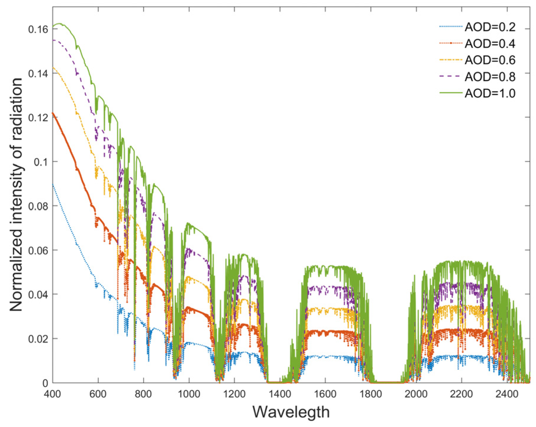
2.1. Atmospheric Radiative Transfer

To calculate the downward radiation term T λ , the UNL-VRTM model is adopted, which is an open-source atmospheric radiative transfer model [38,39]. The inputs of UNL-VRTM include the atmospheric parameters (pressure, altitude, temperature, etc.), aerosol parameters (the aerosol optical depth, particle size distribution, and complex refractive indices), and observation geometries (solar zenith angle, viewing zenith angle, and relative azimuth angle). The outputs of UNL-VRTM include not only the Stokes vector but also their sensitivities (Jacobians) with respect to aerosol and surface model parameters. However, the UNL-VRTM‘s built-in surface model is the kernel-driven BRDF (Bi-directional Reflectance Distribution Function) model, and none of the BRDF kernels contains the phenotypic parameters of the crop. Therefore, the UNL-VRTM model cannot be used directly as a forward model for crop parameter inversion. The main input parameters of the UNL-VRTM model are given in Table 1.

2.2. Crop Canopy Reflectance

The classic PROSAIL model is adopted to describe the contribution of crop canopy R c r o p . The PROSAIL model, a fusion of PROSPECT (leaf reflectance and transmittance) and SAIL (plant canopy reflectance), is widely used for quantitative inversion of vegetation parameters [40,41]. PROSAIL provides the calculation of the spectral and directional reflectance of the plant canopy [42]. However, the application of PROSAIL for crop parameter inversion requires reflectance after atmospheric correction. Traditionally, atmospheric correction is a separate process before inversion, executed by radiative transfer models, such as 6S and RT3. The inputs of the PROSAIL model and the range of parameters are given in Table 2.

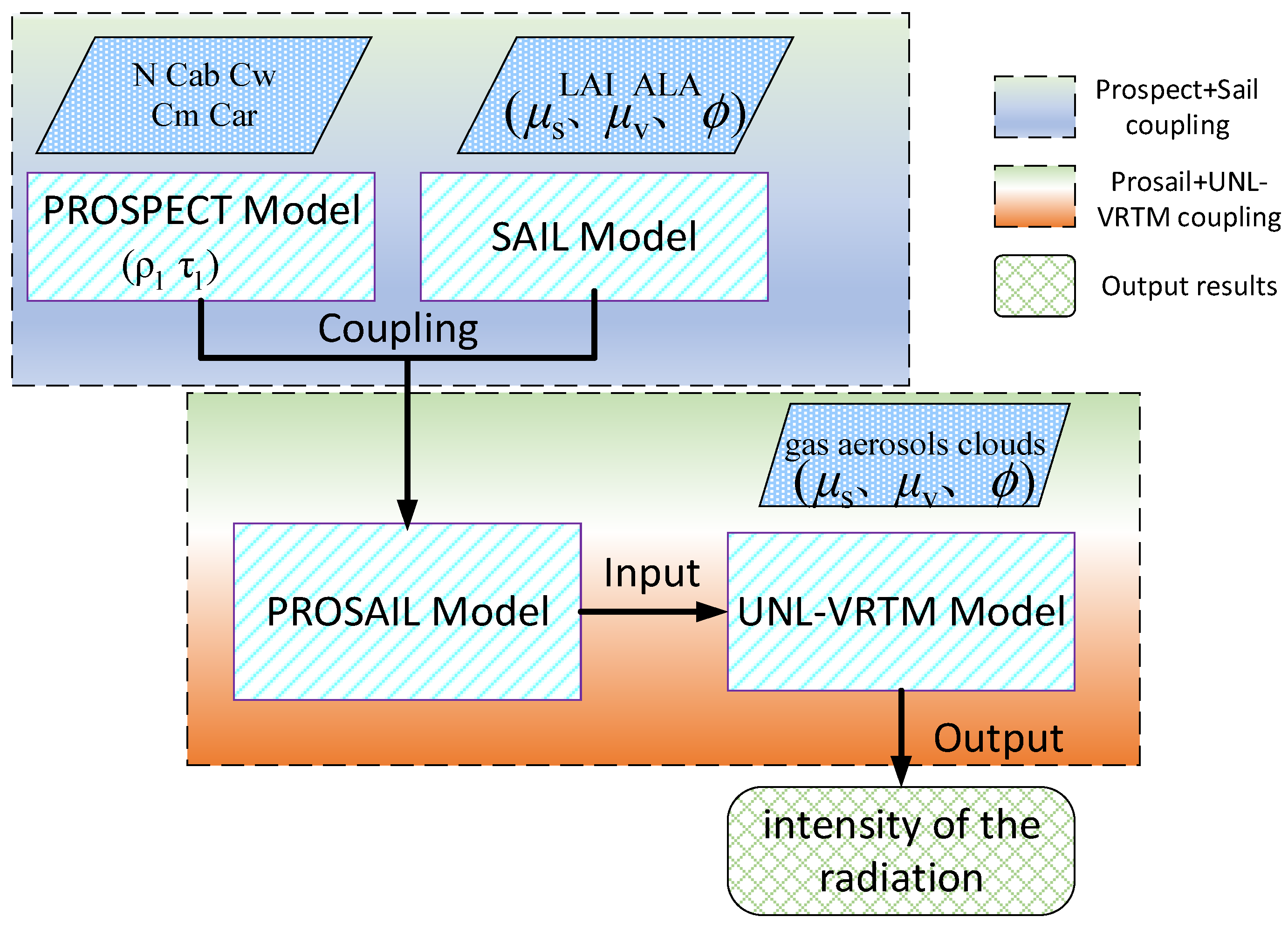
2.3. The Coupling Model for Crop Parameter Inversion

2.3.1. Coupling of Models

For modeling the UAV observations, we replace the built-in surface BRDF (Bidirectional Reflectance Distribution Function) model in UNL-VRTM with the PROSAIL model. Then, the process of atmospheric correction and the process from the biochemical content to the spectral reflectance are integrated into a unified model. The coupling model can be specifically described by the following equation:
M λ μ s , μ v , ϕ = U ( λ , μ s , μ v , ϕ , x a i r , P ( x c r o p ) )
where M denotes the coupling model, U represents the UNL-VRTM model, and P refers to the PROSAIL model. The x a i r and x c r o p represent the atmospheric and crop parameters, respectively.
The diagram of the coupling model is shown in Figure 1. The inputs of the coupling model include the crop physiological parameters, canopy structure parameters, and atmospheric parameters. The output of the coupling model is the intensity of radiation.
The downwelling radiation after gas absorption, Rayleigh scattering, and aerosol scattering, simulated by UNL-VRTM, is shown in Figure 2, in which the assumption of Lambertian surface is adopted, and the surface reflectance is set to 0.2. Moreover, urban aerosol types are selected and different aerosol loadings, of which the AOD (Aerosol optical depth) changes from 0.2 to 1.0, are considered.
It can be seen from Figure 2 that the radiation gradually increased with the increase in AOD on the whole, mainly caused by aerosol scattering. However, the radiation is nearly equal regardless of the AOD in the near-infrared bands (such as 1320–1410 nm and 1800–2200 nm). For the intensity of radiation, it is found that the contribution of AOD has about a 3.0–20% difference with the increase in AOD, indicating that the value of AOD is an important input variable of the UNL-VRTM model.
Based on the values listed in Table 2, the spectral reflectance between 400 nm and 2500 nm, simulated by the PROSAIL model and the coupling model, is shown in Figure 3.
From Figure 3, the reflectance of the coupling model is smaller than the vegetation canopy reflectance simulated by the PROSAIL model at all spectral wavelengths. The decrease in reflectance at wavelengths larger than 750 nm is mainly due to aerosol absorption, and in the blue spectrum (400–450 nm) it is because of the contribution of Rayleigh scattering. Taking into account solar radiation, the spectral reflectance near 1400 and 1900 nm was equal to zero because incident and reflected energy are almost reduced by water vapor and carbon dioxide, which indicated that the forward model has a strong coupling between vegetation canopy and atmosphere environment.

2.3.2. Calculation of Jacobians

The outputs of UNL-VRTM provide the Jacobians of the measurements with respect to the surface reflectance. However, in the inversion framework, the Jacobians of the measurements with respect to the crop phenotype parameter ( x c r o p ) are required. The Jacobian matrix determines the direction of convergence and the step size when solving the cost function [43]. According to the chain rule of derivative, the sensitivity transfer process of the observation vector Y to the crop parameter x c r o p is expressed by the following equation [44,45,46]:
J = Y x c r o p = U P P x c r o p
where U P is the Jacobian of the observation with respect to the canopy reflectance, and P x c r o p is the Jacobian of the canopy reflectance with respect to the crop parameters, which can be calculated by the finite difference method.

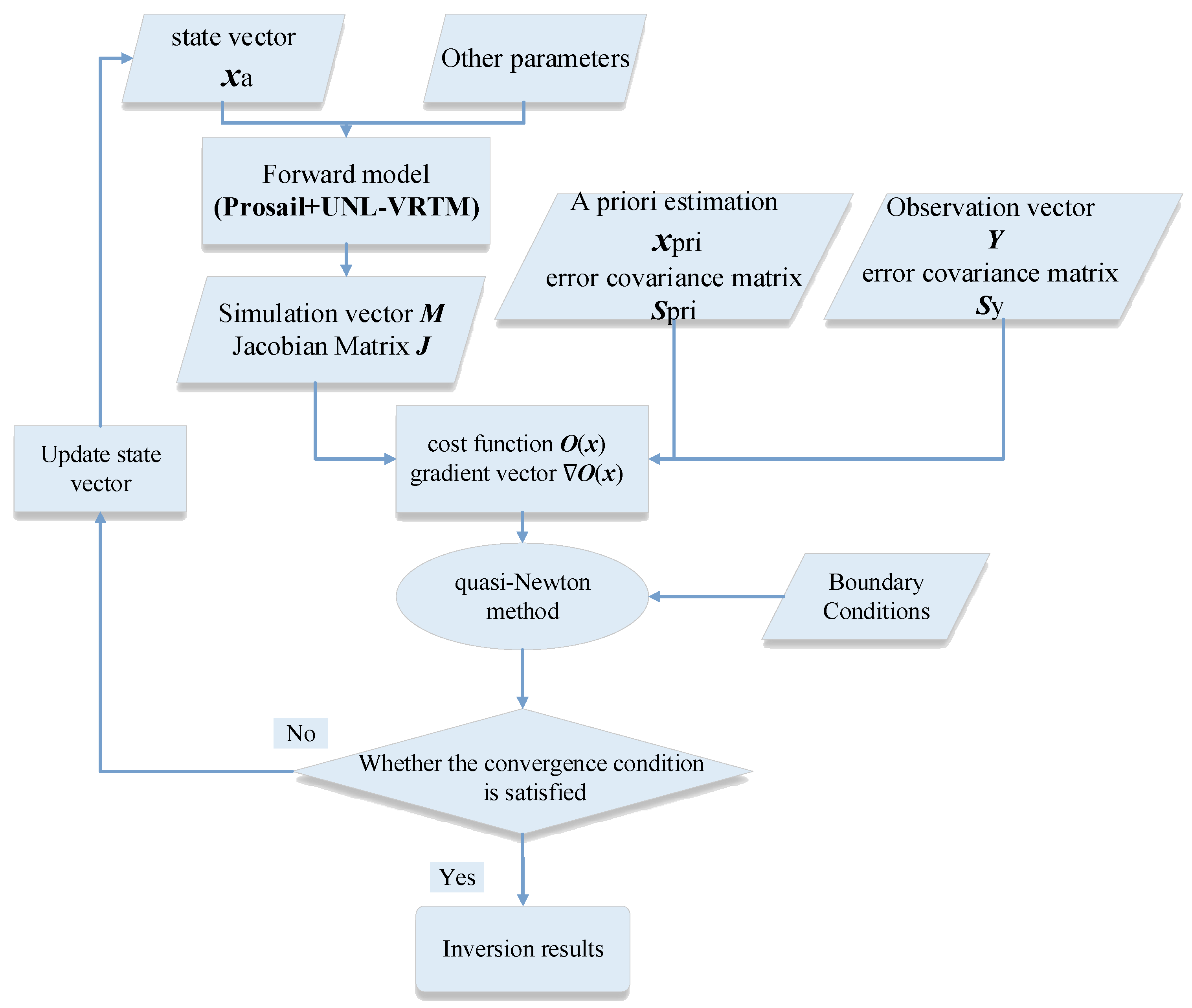
3. Method for the Synchronous Retrieval of LAI and Cab

Inversion is usually defined as determining the state vector by observation vector. A complex UAV observation system can be represented by the simple mathematical model as follows:
Y = M ( x a , x b ) + ϵ
where Y denotes the UAV observation vector and M denotes the forward model. ϵ is an error term including uncertainties in measurements and forward model. x a is the state vector that contains crop parameters to be retrieved, and the choice of state vector depends on which parameter contains more information in the observation data. x b represents other parameters.
The reverse solution of Equation (4) is the inversion process of crop parameters. Assuming that the observed vector can constrain the solution of the above equation, then theoretically x a can be obtained when Y is given. For the UAV observation vector, due to insufficient effective observation information, it is often difficult to constrain the reverse solution process of the above equation. The state vector x a is usually not unique, and we can obtain a statistical estimate value of x a because of the error term ϵ .
Based on the optimal estimation theory, the inversion of crop parameters can be regarded as finding the minimum of the cost function. In most cases, it is an ill-posed problem to find the accurate value of the phenotypic parameters [47]. The a priori knowledge of crop parameters should be introduced into the inversion as a constraint term. Then, the cost function O ( x ) is composed of two terms: the measurement term and a priori constraint term. M is always a nonlinear function for UAV remote sensing, thus solving the optimal solution of Equation (4) needs multiple iterations. The corresponding cost function in the p’th iteration of the state vector is expressed as follows [48,49].
O ( x a p ) = 1 2 [ Y M p ] T S y 1 [ Y M p ] + 1 2 γ ( x a p x p r i ) T S p r i 1 ( x a p x p r i )
where M denotes the simulation results of the forward model at the p’th iteration. S y is the error covariance matrix, which indicates the measurement uncertainty. Lagrange multiplier γ is a regularization parameter defined following the work of Xu et al. [50]. x a p represents the state vector of the p’th iteration. x p r i and S p r i describe the a priori estimate and the error covariance matrix of the state vector, respectively.
Generally, finding the minimum value of O x is a nonlinear problem and needs the gradient vector of O x , which can be further expressed as ∇
O x a p = J T S y 1 Y M p + γ S p r i 1 ( x a p x p r i )
where refers to the gradient operator, and J denotes the Jacobian matrix.
Based on multiple iterations, the state vector at the p + 1′th iteration can be described as:
x a p + 1 = x a p α p H p O ( x a p ) T
where H is the inverse matrix of the Hessian matrix constructed with successive gradient vectors in the quasi-Newton method, and α p is the step factor of the iteration.
The flow chart of the inversion framework is shown in Figure 4. The inputs of the inversion framework include a priori knowledge (prior estimates, upper and lower bounds), the cost function, and its gradient. Firstly, the observation vector Y consists of the hyperspectral or multispectral radiometric measurements carried by the UAV platform, and the observation error covariance matrix S y was constructed by a given observation error. At the same time, the parameters to be retrieved and a priori estimates x p r i should be determined. The error covariance matrix S p r i is constructed according to the uncertainties of a priori estimation. After that, the cost function can be established according to Equation (5). To find the minimum value of O x , the quasi-Newton method implemented by the L-BFGS-B code was introduced. The L-BFGS-B algorithm is a highly effective tool in bounded minimization problems [51,52]. Finally, the optimal estimation of the state vector is considered to be found, if the following Equation (8) is satisfied. Otherwise, the state vector continues to be updated until the termination condition is satisfied. In other words, the crop parameters are retrieved.
x a p + 1 x a p 2 T h r e s h o l d
where   2 denotes the L2 paradigm, and the superscript p refers to the p’th iteration.

4. Model Analysis for UAV Multispectral Measurements

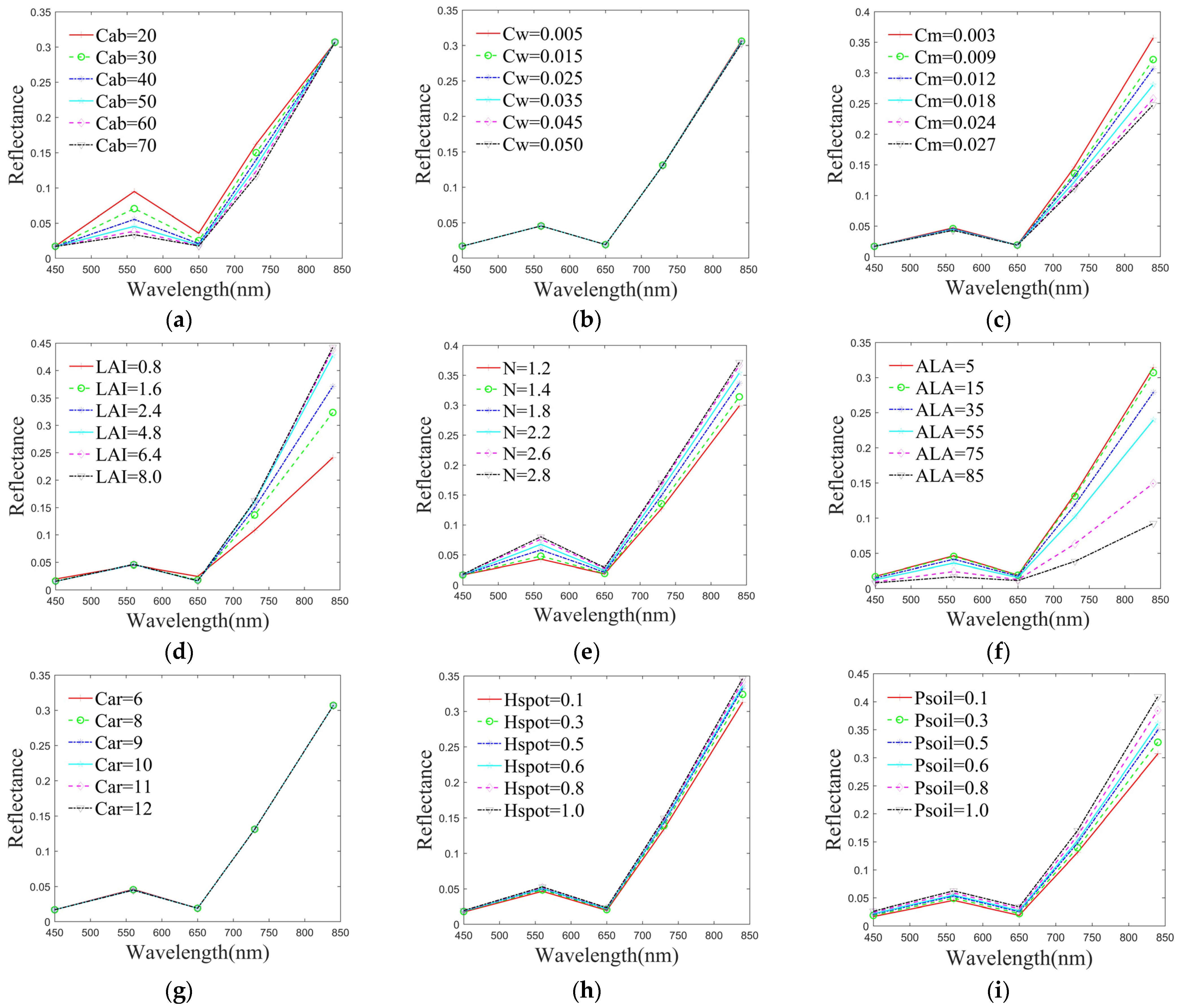
4.1. The Sensitivity of the Model to Crop Parameters

The multispectral sensor is widely used in the agricultural field because of its price advantage. In this paper, the band settings of UAV (P4 Multispectral, SZ DJI Technology Co., Ltd., Shenzhen, China) were adopted, as a case study, for sensitivity analysis of the model to crop parameters. The UAV is equipped with a multispectral camera with the central wavelength of 450, 560, 650, 730, and 840 nm. The band settings of UAV multispectral sensors are given in Table 3.
Obviously, it is difficult to obtain all the crop parameters from the limited channels of the multispectral sensor. Thus, we must figure out exactly which parameter can be retrieved. To solve this problem, firstly, we calculate the influence of each parameter change on the model output reflectance. The simulation results are shown in Figure 5, in which we assumed that the input parameters were independent in the coupling model. For each of the parameters, the reflectance is calculated by fixing other parameter values listed in Table 1 and Table 2.
From Figure 5, we can see that the Cab yields a strong contribution to green band, and a weak influence to red-edge band, and the reflectance gradually decreases with the increase in Cab. It is due to the weak absorption of chlorophyll on the green band. The Cw and Cm reflect the accumulation of water and dry matter during wheat growth, respectively. However, the simulation shows that the sensor is insensitive to Cw in all the channels, and the same is true for the Car parameter on the visible band. The changes of Cm and LAI are well reflected in the reflectance of NIR band, while their contributions are opposite. Parameters related to the structure or geometry, such as the (ALA), leaf structural parameter (N), and Hspot, affect the measurement of all bands. Usually, these parameters are considered as nonstate quantities, using an empirical value with a given error during the inversion. The Psoil represents the proportion of bare soil and vegetation cover; therefore, the increase in Psoil means the enhancement of contribution from the bare soil surface. From Figure 5i, the reflectance of each band increases with the increase in Psoil, since the reflectance of bare soil has little difference at each wavelength. These results were consistent with the previous research [53,54,55].

4.2. Parameters Information Content Analysis

Furthermore, the information of each parameter contained in the multispectral observation is quantified using the degrees of freedom of the signal (DFS) [56]. The DFS is defined as the partial derivative of the posterior estimate values with respect to state parameters and can be calculated by the following equation:
x ^ x = ( J T S O b s 1 J + S p r i 1 ) 1 J T S O b s 1 J
Ideally, the state vector can be completely determined by measurements, that is, all the parameters can be obtained for observation data. In this case, the amount of information for each parameter is equal to 1 and the sum of the information of all parameters is equal to the number of parameters. However, subject to observation and systematic errors, the DFS is always less than 1 for each parameter. Therefore, the signal degrees of freedom can characterize the ability of observations and models to invert parameters. The closer the parameter‘s DFS is to 1, the more adequate information the observation contains about that parameter.
To study the contribution of the phenotypic parameters to observation, Figure 6a shows the variation of all parameters information obtained by different wavelengths’ observation; in other words, the number of parameters can be retrieved from single wavelength observation. In order to describe the observation capabilities of the P4 multispectral UAV, we carried the forward simulation of multispectral bands. Finally, the DFS of each parameter is calculated according to the information content analysis method, as shown in Figure 6b.
From Figure 6a, the total DFS of different wavelengths between 400 and 1200 nm is less than 1, which indicated that the single-band observation has insufficient retrieval ability for multiple parameters. It is because the single band cannot obtain sufficient information. From Figure 6b, (1) the DFS of LAI, Cab, and N were 0.83, 0.71, and 0.58, respectively, significantly higher than Cm (DFS = 0.2). It indicated that the observation contains more effective information on these parameters and can further be better extracted. (2) The DFS of ALA, Car, and Psoil were lower than 0.2, indicating that these parameters are difficult to be retrieved by multispectral observation and can be used as a priori value in the inversion framework.

4.3. Setting of State Vectors and Boundary Conditions

For crop phenotype parameters inversion, we assumed that the observation error does not vary with wavelength and observation geometry in this paper. The state and nonstate vectors of the crop phenotype parameters are composed of the following equations:
x a = C a b , L A I T x b = N , C a r , C w , C m , A L A , h s p o t , p s o i l T
The boundary range of the state vector determines the interval range for finding the optimal solution. The prior estimation is based on the historical data statistics of the same period of crop parameters. The values of the nonstate vector come from the empirical values of the fertility period and sensitivity analysis results, which provide some auxiliary constraints for the optimal solution. In this paper, the boundary conditions for the LAI were (0.5, 7) and for Cab were (20, 70).

5. Results

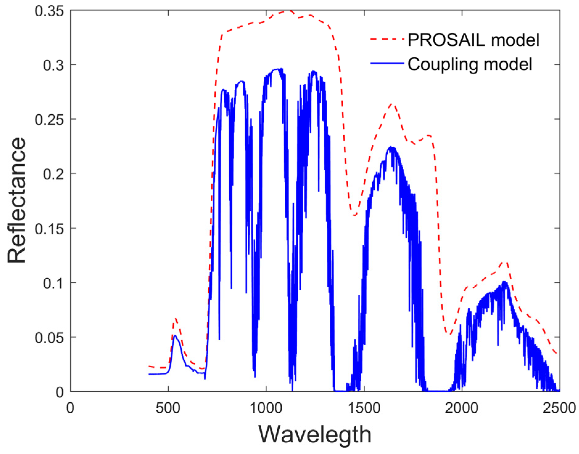
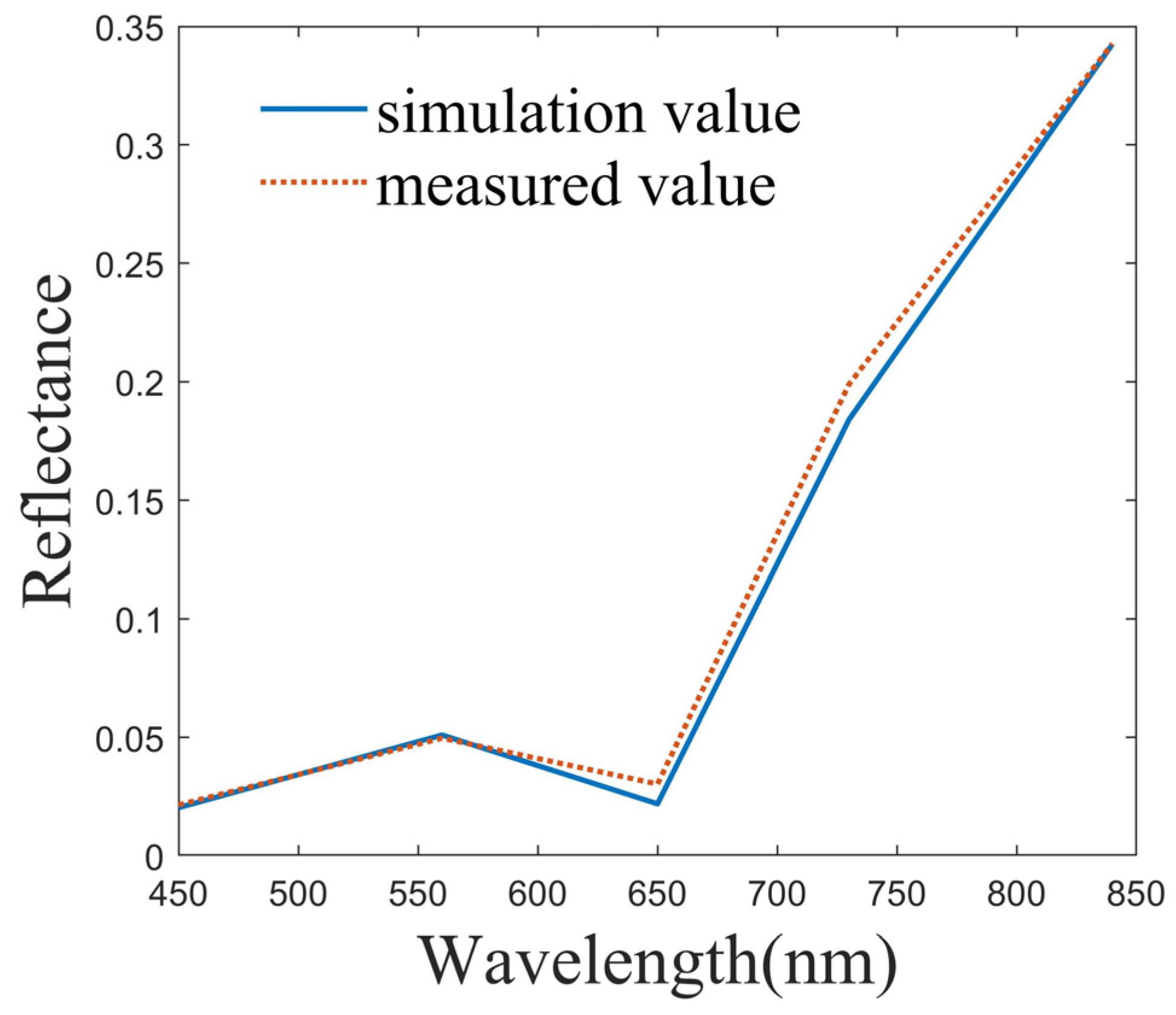
5.1. Validation of the Forward Model

The study area is a national high-standard farmland of 5000 hm2 in Qixian County, Henan Province (114.17° E, 35.6° N), where winter wheat was cultivated annually from October to June, approximately. The region has a warm temperate humid monsoon climate with warm and rainy summer and cold and dry winter. The measured data were derived from the FieldSpec Handheld (a handheld geophysical spectrometer, Analytica Spectra Devices, Inc., Boulder, CO, USA). The spectral range of the measuring instrument is 325~1075 nm, and the spectral resolution was 3 nm at wavelengths 325~700 nm. We collected the test data on 4 March 2021 at about 12:00 when the solar light intensity was stable and the weather was clear and cloudless. The measurement results can represent the true reflectance of the vegetation canopy because the instrument is closer to the target and less influenced by aerosols and water vapor. Figure 7 compares the results between the simulated data at a solar zenith angle of 5° and the measured data at a sampling test point.
It can be seen from Figure 7 that the simulated values of band 3 and band 4 were lower than the ground-measured values. However, the error between the measured and simulated reflectance at the sampling point was within 2%. The results indicated that the simulation of crop reflectance can be achieved by the coupled model from solar radiation to vegetation, further reflecting that the forward modeling process is reasonable.

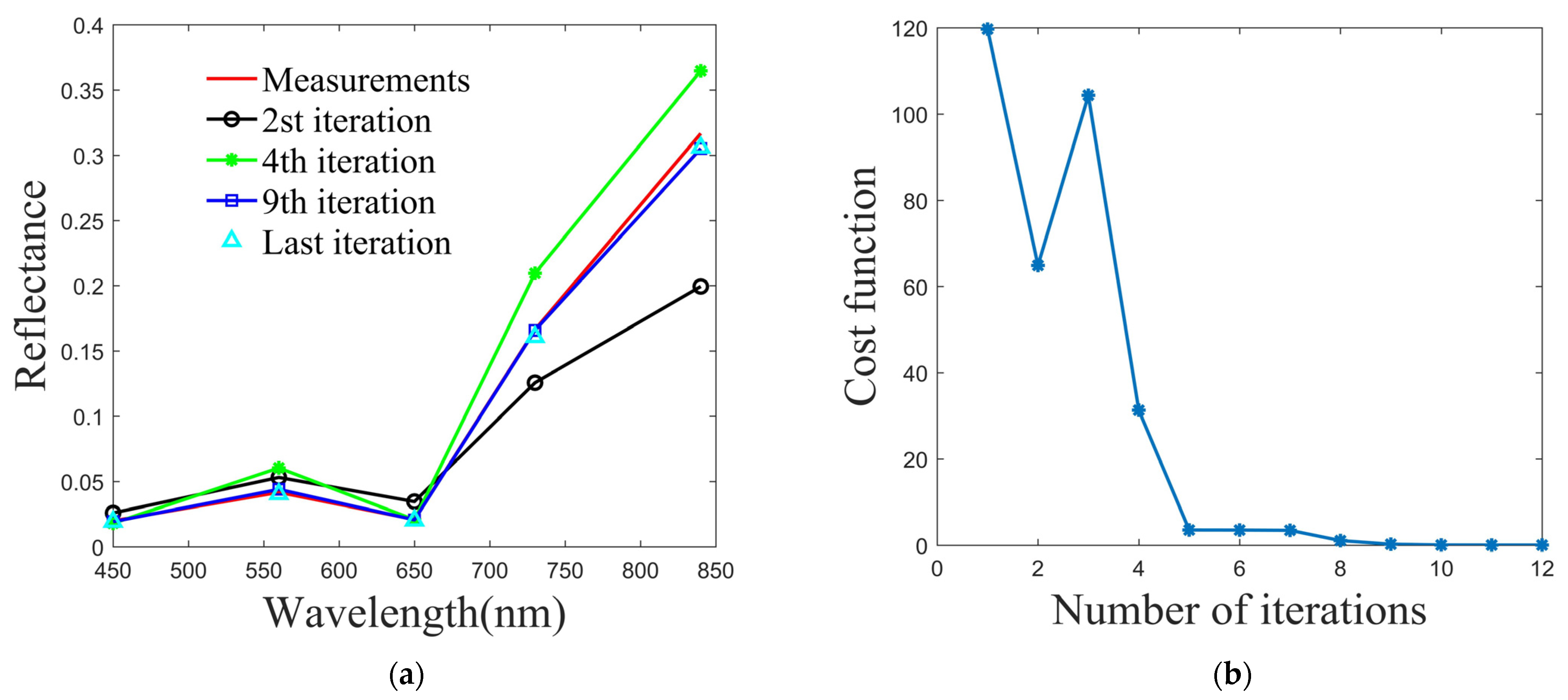
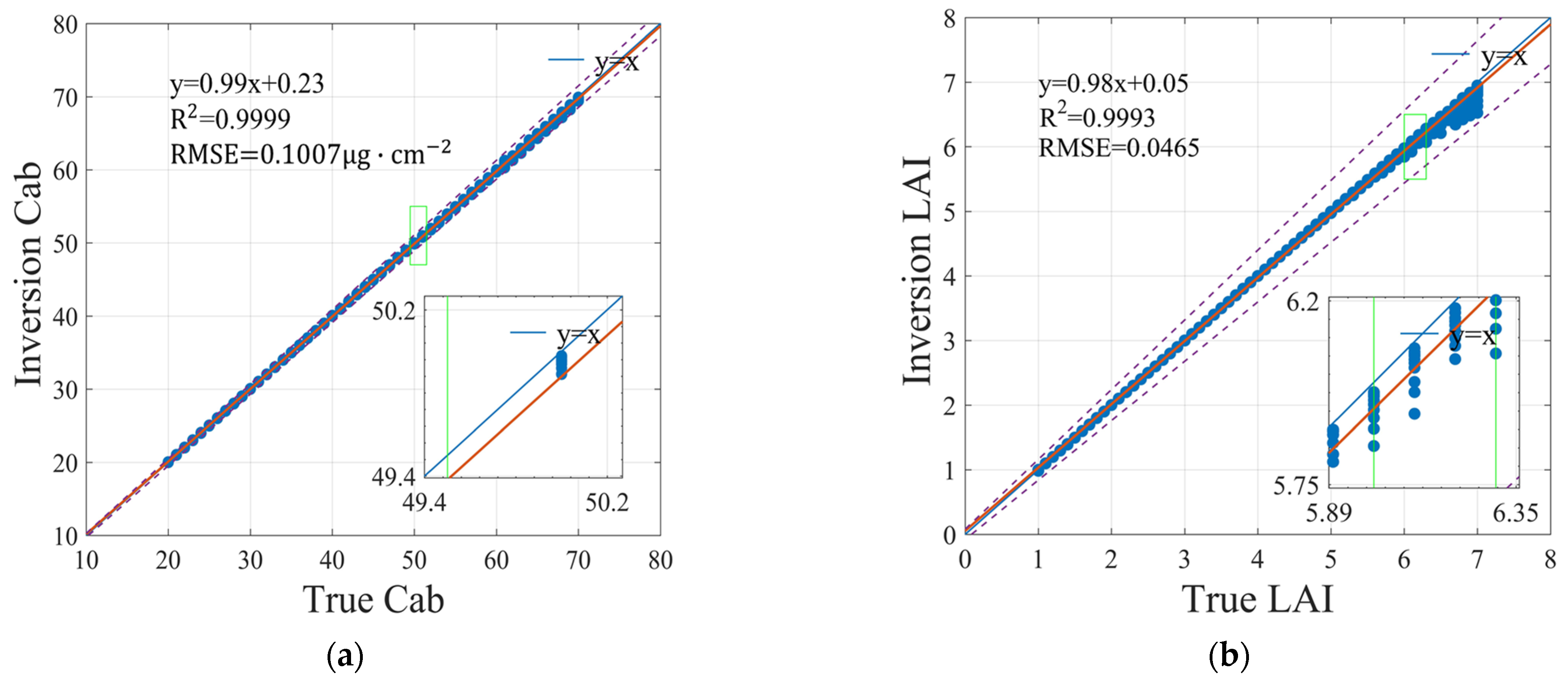
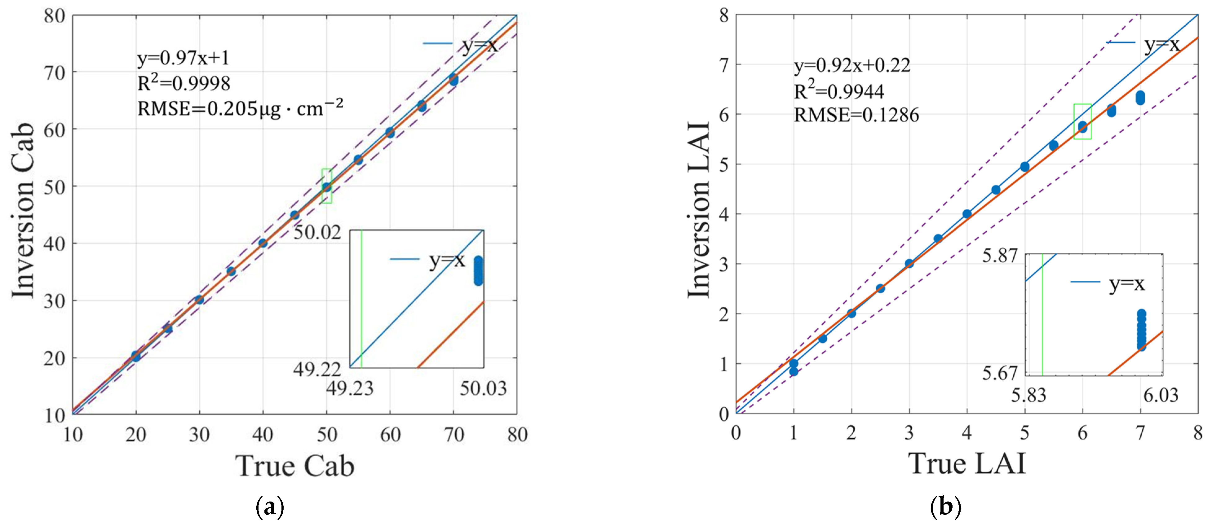
5.2. Retrieval Demonstration and Self-Consistency Tests

Self-consistency tests following the inversion framework are conducted. Firstly, forward simulation datasets are obtained by the coupling model according to the bands of P4 multispectral UAV. The input parameters varied by 10% themselves. The observation geometries are adopted for the yearly solar altitude variation at mid-latitudes in the northern hemisphere [57], in which the solar zenith angle varies from 10° to 60°, view zenith angle and relative azimuth are both 0°. Secondly, to simulate the measurement error, we also added the 5% Gaussian noise to the simulation results. Finally, we obtained a total of 671 sets of validation data.
Figure 8a,b show the iterative process of apparent reflectance and the convergence of cost function for Cab = 63, LAI = 1.3, and the solar zenith angle of 15° in the optimized inversion. The red solid line represents the measured results from the forward model simulation.
As shown in Figure 8a, the model simulated value gradually approaches the observations with the increase in iteration times, and the best fit has been achieved through the OE algorithm at the 14th iteration. The fitting residual error is used to describe the difference between the observation and simulated values. In Figure 8a, the residual error of the last iteration is only 0.023%, and the average residual error of all simulated data is 0.3% after statistics. From Figure 8b, the cost function changes rapidly from the second to the fifth iteration and gradually approached a minimum value after the eighth iteration. The minimum value is determined by the observation error and the error in the radiation transfer and coupling process between the vegetation canopy and the atmosphere. After statistics, the average iteration times of test datasets were about 14 when the cost function reaches the minimum value. The details of the inversion process indicated that the optimal estimation inversion algorithm can realize the dynamic adjustment of inversion parameters and had good convergence in obtaining the retrieval results.
A comparison is summarized in Figure 9 between the inversion values reconstructed from the optimized inversion framework and the true value used in the dataset. The coefficient of determination (R2) and root-mean-square error (RMSE) are used to verify the consistency of the optimized algorithm. A larger R2 and a smaller RMSE indicate the higher accuracy of the forward model and the better consistency of the inversion framework. The retrieved Cab and LAI synchronously under different observation geometries were compared to the true value as shown in Figure 9a,b.
As seen in Figure 9a, the R2 value for Cab was 0.9999, while the RMSE was 0.1007, which indicated that the Cab had good retrieval results. Similarly, the verification results of LAI were consistent with Cab. Meanwhile, it is worth noting that the slopes of the fit lines were all close to 1. With the variation of solar zenith angle, the error lines of Cab and LAI were within E = x ± 0.02x ± 0.08 and E = x ± 0.08x ± 0.08, respectively. The error line is defined as a correlation range between the true value and the inversion value. The results showed the final model retrieval values were in good agreement with the real values.
Moreover, for the validation of the influence of different aerosol loads on the inversion results, another case was also performed. The viewing geometries, including solar zenith angle, view zenith angle, and relative azimuth angle, were 65°, 0°, and 120°, respectively. The state parameters varied by 50% themselves, with different aerosol AOD from 0.1 to 1.0, a total of 130 datasets are obtained. Figure 10a,b show the scatterplots between the retrieval results and the true value under different AODs.
As seen in Figure 10a, the R2 value and RMSE for Cab were 0.9998 and 0.205, which indicated the uncertainty of the retrieved Cab increased weakly with the varying aerosol loading compared with Figure 9a. It can be seen from Figure 10b that the retrieved LAI value is lower than the true value when the LAI is larger than 6. However, the validation results were almost similar to Figure 9a,b, with the R2 values all larger than 0.99. The results indicated that the developed inversion framework showed good performance regardless of the varied aerosol-loading situation.

6. Discussion

The PROSAIL model is sensitive to crop parameters that have been well documented in previous studies [21,40], and UAV-observed reflectance data can in turn promote LAI and Cab retrieval. Nevertheless, solar radiation and atmospheric environment information from UAV observation in physical models cannot be considered in general. Therefore, the forward model by replacing the built-in surface BRDF model in UNL-VRTM with the PROSAIL model was established in this study, which was calculated based on the optimal estimation inversion framework to obtain crop parameters retrieved. The advantage of the forward model is to achieve atmospheric correction during the radiation transfer process and save the costs in human resources, materials, and time. As a result, compared with the measured data collected by the FieldSpec Handheld, the physical transmission model from solar radiation to the crop canopy, and then to the sensor is used as the UAV observation system. Moreover, crop multiparameters retrieved from current inversion approaches cannot be estimated synchronously. Such as LUTs and machine learning algorithms are not suitable for multiparameter inversion [11,27]. Therefore, an optimal estimation inversion algorithm from UAV remote sensing data was proposed, and we can obtain a statistical estimate value of the state vector based on optimal estimation theory. The advantage of the proposed inversion algorithm is that it can extract crop LAI and Cab synchronously from UAV observation.
Based on the optimal estimation theory, we can find the best solution in the continuous state space. Theoretically, the inversion accuracy of crop parameters by the optimal estimation method is higher than LUTs [58]. However, the optimal estimation algorithm requires calculating forward transmission timely and achieves multiple iterations. Thus, it took a lot of time to complete the inversion. After statistics, the average iteration times of test datasets were about 14. We also need to improve the computational efficiency of the inversion algorithm with a larger amount of data.
From the calculation process of the cost function and its gradient vector, it can be seen that our optimal algorithm is related to a priori constraints and the observation data. The algorithm test was carried out based on simulated data in our inversion framework. Although we added noise to the simulated data, the uncertainty of the actual observation data is more complex than the simulated data in fact. The accuracy of the inversion result not only is affected by the uncertainty of observation data, but also depends on prior constraint values (including nonstate parameters value, the initial value of the state parameters, and their boundary conditions). The prior values are derived from historical data statistics of the same period of crop parameters. Reasonable prior estimates and error assumptions can constrain the inversion results to a relatively optimal range and further speed up the iterative computation. Furthermore, we need to optimize the parameter of the measured data and prior constraints and carry out the inversion verification of the actual observation data.

7. Conclusions

In this study, we used a physical model to establish a multiparameter inversion framework for crop phenotypes based on optimal estimation inversion theory. Firstly, we unified PROSAIL and UNL-VRTM models to achieve synchronous atmospheric correction. Secondly, multiple phenotypic parameters inversion framework was established based on the optimized estimation method with prior constraints. Then, the contribution of parameters to the model was obtained by parameter sensitivity analysis, and the parameters to be retrieved were determined according to the information content analysis method. Finally, the optimized estimation inversion framework self-consistency test was performed, and the model inversion values were validated against the true values under different observation geometries and aerosol loadings. The results showed that the coefficients of determination (R2) between the inversion values and the true values were above 0.99, indicating that UAV multispectral observations can support the inversion of LAI and Cab. It also indicated that the inversion framework can make full use of the available radiation spectral information and has good stability. The findings from this study suggest that our proposed forward model has a strong coupling between vegetation reflectance and atmosphere. Moreover, there were good convergence and consistency for the inversion framework in obtaining inversion LAI and Cab. The optimal inversion framework for the synchronous retrieval of crop phenotypic parameters is expected to be performed on actual observation data in the future and can be applied to the monitoring of crop parameters in the field environment.

Author Contributions

Conceptualization, F.Z., J.J. and H.M.; methodology, F.Z. and X.W.; validation, F.Z. and X.W.; formal analysis, F.Z. and J.J.; investigation, F.Z. and X.W.; resources, F.Z., X.W. and S.Z.; data curation, F.Z. and X.W.; writing—original draft preparation, F.Z.; writing—review and editing, F.Z., X.W. and H.C.; supervision, Y.S.; project administration, H.C., Y.S. and J.J.; funding acquisition, J.J. and H.M. All authors have read and agreed to the published version of the manuscript.

Funding

This research was funded by the Key specialized research and development breakthrough in Henan province (No. 222102110105; No. 222102110215); Major science and technology project of Henan Province (No. 221100110800); the Key Scientific Research Projects of Colleges and Universities in Henan Province (No. 21A416003).

Data Availability Statement

Not applicable.

Acknowledgments

We are very grateful to Jun Wang and Xiaoguang Xu for the UNL-VRTM radiative transfer code. The data and Fortran codes used for the forward simulations are available on the UNL-VRTM website (http://www.unl-vrtm.org, accessed on 23 March 2021). We acknowledge the L-BFGS-B software package developed by Ciyou Zhu, Jorge Nocedal, and Richard Byrd.

Conflicts of Interest

The authors declare no conflict of interest.

References

  1. Yang, G.J.; Liu, J.G.; Zhao, C.J.; Li, Z.H.; Huang, Y.B.; Yu, H.Y.; Xu, B.; Yang, X.D.; Zhu, D.M.; Zhang, X.Y.; et al. Unmanned aerial vehicle remote sensing for field-based crop phenotyping: Current status and perspectives. Front. Plant Sci. 2017, 8, 1111. [Google Scholar] [CrossRef] [PubMed] [Green Version]
  2. Zhang, H.D.; Wang, L.Q.; Tian, T.; Yin, J.H. A review of unmanned aerial vehicle low-altitude remote sensing (uav-lars) use in agricultural monitoring in China. Remote Sens. 2021, 13, 1221. [Google Scholar] [CrossRef]
  3. Tattaris, M.; Reynolds, M.P.; Chapman, S.C. A direct comparison of remote sensing approaches for high-throughput phenotyping in plant breeding. Front. Plant Sci. 2016, 7, 1131. [Google Scholar] [CrossRef]
  4. Haghighattalab, A.; Perez, L.G.; Mondal, S.; Singh, D.; Schinstock, D.; Rutkoski, J.; Ortiz-Monasterio, I.; Singh, R.P.; Goodin, D.; Poland, J. Application of unmanned aerial systems for high throughput phenotyping of large wheat breeding nurseries. Plant Methods 2016, 12, 35. [Google Scholar] [CrossRef] [PubMed] [Green Version]
  5. Gracia-Romero, A.; Kefauver, S.C.; Fernandez-Gallego, J.A.; Vergara-Diaz, O.; Nieto-Taladriz, M.T.; Araus, J.L. UAV and ground image-based phenotyping: A proof of concept with durum wheat. Remote Sens. 2019, 11, 1244. [Google Scholar] [CrossRef] [Green Version]
  6. Tao, H.L.; Feng, H.K.; Xu, L.J.; Miao, M.K.; Long, H.L.; Yue, J.B.; Li, Z.H.; Yang, G.J.; Yang, X.D.; Fan, L.L. Estimation of crop growth parameters using UAV-based hyperspectral remote sensing data. Sensors 2020, 20, 1296. [Google Scholar] [CrossRef] [Green Version]
  7. Feng, A.J.; Zhou, J.F.; Vories, E.D.; Sudduth, K.A.; Zhang, M.N. Yield estimation in cotton using UAV-based multi-sensor imagery. Biosyst. Eng. 2020, 193, 101–114. [Google Scholar] [CrossRef]
  8. Ma, C.Y.; Liu, M.X.; Ding, F.; Li, C.C.; Cui, Y.Q.; Chen, W.N.; Wang, Y.L. Wheat growth monitoring and yield estimation based on remote sensing data assimilation into the SAFY crop growth model. Sci. Rep. 2022, 12, 5473. [Google Scholar] [CrossRef]
  9. Velusamy, P.; Rajendran, S.; Mahendran, R.K.; Naseer, S.; Shafiq, M.; Choi, J.G. Unmanned aerial vehicles (UAV) in precision agriculture: Applications and challenges. Energies 2022, 15, 217. [Google Scholar] [CrossRef]
  10. Liu, K.; Zhou, Q.B.; Wu, W.B.; Tian, X.; Tang, H.J. Estimating the crop leaf area index using hyperspectral remote sensing. J. Integr. Agric. 2016, 15, 475–491. [Google Scholar] [CrossRef] [Green Version]
  11. Darvishzadeh, R.; Atzberger, C.; Skidmore, A.; Schlerf, M. Mapping grassland leaf area index with airborne hyperspectral imagery: A comparison study of statistical approaches and inversion of radiative transfer models. ISPRS J. Photogramm. Remote Sens. 2011, 66, 894–906. [Google Scholar] [CrossRef]
  12. Liang, L.; Huang, T.; Di, L.P.; Geng, D.; Di, G.; Yan, J.; Wang, S.G.; Wang, L.J.; Li, L.; Chen, B.Q.; et al. Influence of different bandwidths on LAI estimation using vegetation indices. IEEE J. Sel. Top. Appl. Earth Obs. Remote Sens. 2020, 13, 1494–1502. [Google Scholar] [CrossRef]
  13. Viña, A.; Gitelson, A.A.; Nguy-Robertson, A.L.; Peng, Y. Comparison of different vegetation indices for the remote assessment of green leaf area index of crops. Remote Sens. Environ. 2011, 115, 3468–3478. [Google Scholar] [CrossRef]
  14. Yu, K.; Lenz-Wiedemann, V.; Chen, X.P.; Bareth, G. Estimating leaf chlorophyll of barley at different growth stages using spectral indices to reduce soil background and canopy structure effects. ISPRS J. Photogramm. Remote Sens. 2014, 97, 58–77. [Google Scholar] [CrossRef]
  15. Lin, H.; Liang, L.; Zhang, L.P.; Du, P.J. Wheat leaf area index inversion with hyperspectral remote sensing based on support vector regression algorithm. Trans. Chin. Soc. Agric. Eng. 2013, 29, 139–146. [Google Scholar]
  16. Liang, L.; Di, L.P.; Zhang, L.P.; Deng, M.X.; Qin, Z.H.; Zhao, S.H.; Lin, H. Estimation of crop LAI using hyperspectral vegetation indices and a hybrid inversion method. Remote Sens. Environ. 2015, 165, 123–134. [Google Scholar] [CrossRef]
  17. Verrelst, J.; Muñoz, J.; Alonso, L.; Delegido, J.; Rivera, J.P.; Camps-Valls, G.; Moreno, J. Machine learning regression algorithms for biophysical parameter retrieval: Opportunities for sentinel-2 and -3. Remote Sens. Environ. 2012, 118, 127–139. [Google Scholar] [CrossRef]
  18. Lu, X.P.; Wang, X.X.; Zhang, X.J.; Wang, J.; Yang, Z.N. Winter wheat leaf area index inversion by the genetic algorithms neural network model based on SAR data. Int. J. Digit. Earth 2022, 15, 362–380. [Google Scholar] [CrossRef]
  19. Saddik, A.; Latif, R.; Elhoseny, M.; El Ouardi, A. Real-time evaluation of different indexes in precision agriculture using a heterogeneous embedded system. Sustain. Comput. Inform. Syst. 2021, 30, 100506. [Google Scholar] [CrossRef]
  20. Saddik, A.; Latif, R.; El Ouardi, A.; Alghamdi, M.I.; Elhoseny, M. Improving Sustainable Vegetation Indices Processing on Low-Cost Architectures. Sustainability 2022, 14, 2521. [Google Scholar] [CrossRef]
  21. Duan, S.B.; Li, Z.L.; Wu, H.; Tang, B.H.; Ma, L.L.; Zhao, E.Y.; Li, C.R. Inversion of the PROSAIL model to estimate leaf area index of maize, potato, and sunflower fields from unmanned aerial vehicle hyperspectral data. Int. J. Appl. Earth Obs. Geoinf. 2014, 26, 12–20. [Google Scholar] [CrossRef]
  22. Upreti, D.; Huang, W.J.; Kong, W.P.; Pascucci, S.; Pignatti, S.; Zhou, X.F.; Ye, H.C.; Casa, R. A comparison of hybrid machine learning algorithms for the retrieval of wheat biophysical variables from sentinel-2. Remote Sens. 2019, 11, 481. [Google Scholar] [CrossRef] [Green Version]
  23. Rivera, J.P.; Verrelst, J.; Leonenko, G.; Moreno, J. Multiple cost functions and regularization options for improved retrieval of leaf chlorophyll content and LAI through Inversion of the PROSAIL Model. Remote Sens. 2013, 5, 3280–3304. [Google Scholar] [CrossRef] [Green Version]
  24. He, W.; Yang, H.; Pan, J.J.; Xu, P.P. Exploring Optimal Design of Look-Up Table for PROSAIL Model Inversion with Multi-Angle MODIS Data. In Proceedings of the Land Surface Remote Sensing, Kyoto, Japan, 21 November 2012; SPIE: Bellingham, WA, USA, 2012; Volume 8524, pp. 327–339. [Google Scholar]
  25. Richter, K.; Hank, T.B.; Vuolo, F.; Mauser, W.; D’Urso, G. Optimal exploitation of the sentinel-2 spectral capabilities for crop leaf area index mapping. Remote Sens. 2012, 4, 561–582. [Google Scholar] [CrossRef] [Green Version]
  26. Sun, J.; Wang, L.; Shi, S.; Li, Z.H.; Yang, J.; Gong, W.; Wang, S.Q.; Tagesson, T. Leaf pigment retrieval using the PROSAIL model: Influence of uncertainty in prior canopy-structure information. Crop J. 2022, 10, 1251–1263. [Google Scholar] [CrossRef]
  27. Miraglio, T.; Adeline, K.; Huesca, M.; Ustin, S.; Briottet, X. Joint use of PROSAIL and DART for fast LUT building: Application to gap fraction and leaf biochemistry estimations over sparse oak stands. Remote Sens. 2020, 12, 2925. [Google Scholar] [CrossRef]
  28. Darvishzadeh, R.; Matkan, A.A.; Ahangar, A.D. Inversion of a radiative transfer model for estimation of rice canopy chlorophyll content using a lookup-table approach. IEEE J. Sel. Top. Appl. Earth Obs. Remote Sens. 2012, 5, 1222–1230. [Google Scholar] [CrossRef]
  29. Sun, B.; Wang, C.F.; Yang, C.H.; Xu, B.D.; Zhou, G.S.; Li, X.Y.; Xie, J.; Xu, S.J.; Liu, B.; Zhang, J.; et al. Retrieval of rapeseed leaf area index using the PROSAIL model with canopy coverage derived from UAV images as a correction parameter. Int. J. Appl. Earth Obs. Geoinf. 2021, 102, 102373. [Google Scholar] [CrossRef]
  30. Berger, K.; Atzberger, C.; Danner, M.; D’Urso, G.; Mauser, W.; Vuolo, F.; Hank, T. Evaluation of the PROSAIL model capabilities for future hyperspectral model environments: A review study. Remote Sens. 2018, 10, 85. [Google Scholar] [CrossRef] [Green Version]
  31. Bassani, C.; Sterckx, S. Calibration of satellite low radiance by AERONET-OC products and 6SV model. Remote Sens. 2021, 13, 781. [Google Scholar] [CrossRef]
  32. Rosas, J.; Houborg, R.; McCabe, M.F. Sensitivity of Landsat 8 surface temperature estimates to atmospheric profile data: A study using MODTRAN in dryland irrigated systems. Remote Sens. 2017, 9, 988. [Google Scholar] [CrossRef] [Green Version]
  33. Shang, H.; Chen, L.; Breon, F.M.; Letu, H.; Li, S.; Wang, Z.; Su, L. Impact of cloud horizontal inhomogeneity and directional sampling on the retrieval of cloud droplet size by the POLDER instrument. Atmos. Meas. Tech. 2015, 8, 4931–4945. [Google Scholar] [CrossRef] [Green Version]
  34. Zheng, F.X. Aerosol Multi-Parameter Optimal Retrieval from Multi-Angle Polarization Satellite Data; University of Chinese Academy of Sciences: Beijing, China, 2019. [Google Scholar]
  35. Gómez-Dans, J.L.; Lewis, P.E.; Disney, M. Efficient emulation of radiative transfer codes using gaussian processes and application to land surface parameter inferences. Remote Sens. 2016, 8, 119. [Google Scholar] [CrossRef] [Green Version]
  36. Mishchenko, M.I.; Travis, L.D.; Lacis, A.A. Scattering, Absorption, and Emission of Light by Small Particles; Cambridge University Press: Cambridge, UK, 2002. [Google Scholar]
  37. Kaufman, Y.J.; Tanré, D.; Gordon, H.R.; Nakajima, T.; Lenoble, J.; Frouin, R.; Grassl, H.; Herman, B.M.; King, M.D.; Teillet, P.M. Passive remote sensing of tropospheric aerosol and atmospheric correction for the aerosol effect. J. Geophys. Res. Atmos. 1997, 102, 16815–16830. [Google Scholar] [CrossRef] [Green Version]
  38. Hou, W.; Li, Z.; Wang, J.; Xu, X.; Goloub, P.; Qie, L. Improving remote sensing of aerosol microphysical properties by near-infrared polarimetric measurements over vegetated land: Information content analysis. J. Geophys. Res. Atmos. 2018, 123, 2215–2243. [Google Scholar] [CrossRef]
  39. Wang, J.; Xu, X.G.; Ding, S.G.; Zeng, J.; Spurr, R.; Liu, X.; Chance, K.; Mishchenko, M. A numerical testbed for remote sensing of aerosols, and its demonstration for evaluating retrieval synergy from a geostationary satellite constellation of GEO-CAPE and GOES-R. J. Quant. Spectrosc. Radiat. Transf. 2014, 146, 510–528. [Google Scholar] [CrossRef] [Green Version]
  40. Adeluyi, O.; Harris, A.; Verrelst, J.; Foster, T.; Clay, G.D. Estimating the phenological dynamics of irrigated rice leaf area index using the combination of PROSAIL and gaussian process regression. Int. J. Appl. Earth Obs. Geoinf. 2021, 102, 102454. [Google Scholar] [CrossRef]
  41. Jacquemoud, S.; Verhoef, W.; Baret, F.; Bacour, C.; Zarco-Tejada, P.J.; Asner, G.P.; François, C.; Ustin, S.L. PROSPECT+SAIL models: A review of use for vegetation characterization. Remote Sens. Environ. 2009, 113, S56–S66. [Google Scholar] [CrossRef]
  42. Tripathi, R.; Sahoo, R.N.; Sehgal, V.K.; Tomar, R.K.; Chakraborty, D.; Nagarajan, S. Inversion of PROSAIL model for retrieval of plant biophysical parameters. J. Indian Soc. Remote Sens. 2012, 40, 19–28. [Google Scholar] [CrossRef]
  43. Hou, W.; Wang, J.; Xu, X.; Reid, J.S.; Han, D. An algorithm for hyperspectral remote sensing of aerosols: 1. Development of theoretical framework. J. Quant. Spectrosc. Radiat. Transf. 2016, 178 (Suppl. C), 400–415. [Google Scholar] [CrossRef]
  44. Zheng, F.X.; Li, Z.Q.; Hou, W.Z.; Qie, L.L.; Zhang, C. Aerosol retrieval study from multiangle polarimetric satellite data based on optimal estimation method. J. Appl. Remote Sens. 2020, 14, 014516. [Google Scholar] [CrossRef]
  45. Zheng, F.X.; Hou, W.Z.; Li, Z.Q. Improvement of Aerosol Fine Mode Fraction Retrieval from Skylight Measurements by Degree of Linear Polarization: Information Content Analysis. In Proceedings of the AOPC 2020: Optical Spectroscopy and Imaging; and Biomedical Optics, Beijing, China, 5 November 2020; SPIE: Bellingham, WA, USA, 2020; Volume 11566, p. 1156602. [Google Scholar]
  46. Spurr, R.; Wang, J.; Zeng, J.; Mishchenko, M.I. Linearized T-matrix and Mie scattering computations. J. Quant. Spectrosc. Radiat. Transf. 2012, 113, 425–439. [Google Scholar] [CrossRef] [Green Version]
  47. Combal, B.; Baret, F.; Weiss, M.; Trubuil, A.; Macé, D.; Pragnère, A.; Myneni, R.; Knyazikhin, Y.; Wang, L. Retrieval of canopy biophysical variables from bidirectional reflectance. Remote Sens. Environ. 2003, 84, 1–15. [Google Scholar] [CrossRef]
  48. Dubovik, O.; Herman, M.; Holdak, A.; Lapyonok, T.; Tanré, D.; Deuzé, J.L.; Ducos, F.; Sinyuk, A.; Lopatin, A. Statistically optimized inversion algorithm for enhanced retrieval of aerosol properties from spectral multi-angle polarimetric satellite observations. Atmos. Meas. Tech. 2011, 4, 975–1018. [Google Scholar] [CrossRef] [Green Version]
  49. Wu, L.; Hasekamp, O.; Van Diedenhoven, B.; Cairns, B. Aerosol retrieval from multiangle, multispectral photopolarimetric measurements: Importance of spectral range and angular resolution. Atmos. Meas. Tech. 2015, 8, 2625–2638. [Google Scholar] [CrossRef] [Green Version]
  50. Xu, X.G.; Wang, J. Retrieval of aerosol microphysical properties from AERONET photopolarimetric measurements: 1. Information content analysis. J. Geophys. Res. Atmos. 2015, 120, 7059–7078. [Google Scholar] [CrossRef] [Green Version]
  51. Byrd, R.H.; Lu, P.H.; Nocedal, J.; Zhu, C.Y. A limited memory algorithm for bound constrained optimization. SIAM J. Sci. Comput. 1995, 16, 1190–1208. [Google Scholar] [CrossRef]
  52. Xiao, Y.H.; Zhang, H.C. Modified subspace limited memory BFGS algorithm for large-scale bound constrained optimization. J. Comput. Appl. Math. 2008, 222, 429–439. [Google Scholar] [CrossRef] [Green Version]
  53. Su, W.; Wu, J.Y.; Wang, X.S.; Xie, Z.X.; Zhang, Y.; Tao, W.C.; Jin, T. Retrieving corn canopy leaf area index based on sentinel-2 image and PROSAIL model parameter calibration. Spectrosc. Spectr. Anal. 2021, 41, 1891–1897. [Google Scholar]
  54. Jia, J.Q. Study on the Inversion Method of Leaf Area Index of Summer Maize at Different Growth Stages Based on GF-2 Satellite. Northwest University: Kirkland, WA, USA, 2018. [Google Scholar]
  55. Wan, L.; Zhang, J.F.; Dong, X.Y.; Du, X.Y.; Zhu, J.P.; Sun, D.W.; Liu, Y.F.; He, Y.; Cen, H.Y. Unmanned aerial vehicle-based field phenotyping of crop biomass using growth traits retrieved from PROSAIL model. Comput. Electron. Agric. 2021, 187, 106304. [Google Scholar] [CrossRef]
  56. Hou, W.Z.; Wang, J.; Xu, X.G.; Reid, J.S. An algorithm for hyperspectral remote sensing of aerosols: 2. Information content analysis for aerosol parameters and principal components of surface spectra. J. Quant. Spectrosc. Radiat. Transf. 2017, 192 (Suppl. C), 14–29. [Google Scholar] [CrossRef]
  57. Wang, G.A.; Mi, H.T.; Deng, T.H.; Li, Y.N.; Li, L.X. Calculation of the change range of the sun high angle and the azimuth of sunrise and sunset in one year. Meteorol. Environ. Sci. 2007, 30, 161–164. [Google Scholar]
  58. Jeong, U.; Kim, J.; Ahn, C.; Torres, O.; Liu, X.; Bhartia, P.K.; Spurr, R.J.; Haffner, D.; Chance, K.; Holben, B.N. An optimal-estimation-based aerosol retrieval algorithm using OMI near-UV observations. Atmos. Chem. Phys. 2016, 16, 177–193. [Google Scholar] [CrossRef] [Green Version]
Figure 1. Diagram of the coupling model (where μ s and μ v are cosine of solar zenith angle and cosine of view zenith angle, respectively, and ϕ is relative azimuth angle.)
Agronomy 13 01119 g001
Figure 2. Forward simulation of different atmospheric aerosols by UNL-VRTM.
Agronomy 13 01119 g002
Figure 3. The spectral reflectance simulated by PROSAIL and the coupling model.
Agronomy 13 01119 g003
Figure 4. The optimization inversion flow chart based on iteration.
Agronomy 13 01119 g004
Figure 5. Spectral response under different input parameter values. (ad) are the different reflectance changes of physicochemical parameters Cab, Cw, Cm and LAI, respectively. (e,f) are the difference reflectance changes of structure parameter N and geometry parameter ALA, respectively. (gi) are the difference reflectance changes of parameters Car, Hspot and Psoil, respectively.
Agronomy 13 01119 g005
Figure 6. The DFS of crop parameters: (a) the DFS of different wavelengths for all parameters and (b) the DFS of five bands for each parameter.
Agronomy 13 01119 g006
Figure 7. Comparison of simulated values and ground truth values.
Agronomy 13 01119 g007
Figure 8. Retrieval process demonstration: (a) the illustration of the iterative process for reflectance based on the coupling model and (b) the description of the convergence process for the cost function.
Agronomy 13 01119 g008
Figure 9. Validation of the Cab and LAI with the OE-iteration method: (a) validation of the Cab with the OE-iteration method against the true value under different observation geometries and (b) validation of the LAI with the OE-iteration method against the true value under different observation geometries. The blue solid line, dashed line, and orange solid line are the 1:1 line, error line, and fit line, respectively. The error lines of (a,b) are E = x ± 0.02x ± 0.08 and E = x ± 0.08x ± 0.08. The statistics of the linear fitting result, including slope, intercept, R2, and RMSE, are listed in the upper left corner of each scatter plot.
Agronomy 13 01119 g009
Figure 10. Validation of the Cab and LAI with the OE-iteration method: (a) validation of the Cab with the OE-iteration method against the true value under different AODs and (b) validation of the LAI with the OE-iteration method against the true value under different AODs. The blue solid line, dashed line, and orange solid line are the 1:1 line, error line, and fit line, respectively. The error lines of (a,b) are E = x ± 0.04x ± 0.08.and E = x ± 0.14x ± 0.08. The statistics of the linear fitting result, including slope, intercept, R2, and RMSE, are listed in the upper left corner of each scatter plot.
Agronomy 13 01119 g010
Table 1. Main input parameters of the UNL-VRTM model.
Parameter TypesParameter SymbolsParameter DescriptionUnit
GeometrySZASolar zenith angleDegrees (°)
VZAViewing zenith angleDegrees (°)
SAASolar azimuthal angleDegrees (°)
VAAViewing azimuthal angleDegrees (°)
AtmosphereAtmospheric typeThe meteorological and air density profile--
PressureSurface pressurehPa
AltitudeSurface altitudem
AerosolAODAerosol optical depth--
RiComplex refractive index of aerosol--
ProfileThe vertical profile of aerosol--
PSDAerosol particle size distribution--
SurfaceLambertianLambertian surface reflectance--
BRDFSurface bidirectional reflectance--
SpectraWavelengthCentral wavelength of spectral channelnm
FWHMFull width at half maximum of spectral channelnm
Table 2. Main input parameters of the PROSAIL model.
ModelParameter SymbolsParameter DescriptionCommon ValueSearch RangeUnit
PROSPECTNLeaf structure parameter1.31.2~2.8--
CabChlorophyll a and b content5020~70μg·cm−2
CarCarotenoids content86~12μg·cm−2
CwEquivalent water thickness0.0040.004~0.05cm
CmLeaf mass per unit leaf area0.0120.003~0.027g·cm−2
SAILLAILeaf area index1.41~7--
ALAAverage leaf angle150~90Degrees (°)
HspotHot spot0.010.01~1.0--
PsoilSoil coefficient0.10.1~1.0--
Table 3. The multispectral bands of UAV.
BandCenter Wavelength/nmBandwidth
Band1-Blue45016
Band2-Green56016
Band3-Red65016
Band4-RedEdge73016
Band5-NIR84026
Disclaimer/Publisher’s Note: The statements, opinions and data contained in all publications are solely those of the individual author(s) and contributor(s) and not of MDPI and/or the editor(s). MDPI and/or the editor(s) disclaim responsibility for any injury to people or property resulting from any ideas, methods, instructions or products referred to in the content.

