Article

Toward Sustainable Farming: Implementing Artificial Intelligence to Predict Optimum Water and Energy Requirements for Sensor-Based Micro Irrigation Systems Powered by Solar PV

1
Date Palm Research Center of Excellence, King Faisal University, Al-Ahsa 31982, Saudi Arabia
2
Department of Agricultural and Biosystems Engineering, Faculty of Agriculture, Menoufia University, Shebin El Koum 32514, Egypt
3
Center for Artificial Intelligence and Robotics (CAIRO), Aswan University, Aswan 81582, Egypt
4
College of Computer Sciences and Information Technology, King Faisal University, Al-Ahsa 31982, Saudi Arabia
*
Author to whom correspondence should be addressed.
Agronomy 2023, 13(4), 1081; https://doi.org/10.3390/agronomy13041081
Submission received: 15 March 2023 / Revised: 6 April 2023 / Accepted: 7 April 2023 / Published: 8 April 2023
(This article belongs to the Special Issue Agricultural Automation and Innovative Agricultural Systems)

Abstract

:
Future trends in climate change, water scarcity, and energy costs will motivate agriculturists to develop innovative agricultural systems. In order to achieve sustainable farming in arid regions, there is an urgent need to use artificial intelligence (AI) to predict and estimate the optimum water and energy requirements for the irrigation of date palms. Therefore, this study aimed to predict the optimum water and energy requirements for date palm irrigation depending on the optimum water use efficiency (WUE) and yield in arid conditions. To achieve this aim, four solar-powered micro irrigation systems were developed and evaluated under six irrigation levels for date palm irrigation. Soil moisture sensor-based controllers were used to automate irrigation scheduling for the micro irrigation systems. The water pumping in these systems was powered using a solar photovoltaic (PV) system. In addition, four machine-learning (ML) algorithms, including linear regression (LR), support vector regression (SVR), long short-term memory (LSTM) neural network, and extreme gradient boosting (XGBoost), were developed and validated for prediction purposes. These models were developed in Python programing language using the Keras library. The results indicated that the optimum WUS was achieved when the maximum setpoints of irrigation control were adjusted at the field capacity and by adjusting the minimum setpoints at 40, 50, 70, and 80% of the available water (AW). The optimum yield was achieved by adjusting the minimum setpoints at 60, 70, 80, and 90% of AW for subsurface irrigation, subsurface drip irrigation, drip irrigation, and bubbler irrigation, respectively. Therefore, the dataset was prepared at these levels for four years to train and test the models, and a fifth year was used to validate the performance of the best model. The evaluation of the models showed that the LSTM followed by XGBoost models were more accurate than the SVR and LR models for predicting the optimum irrigation water and energy requirements. The validation result showed that the LSTM was able to predict the water and energy requirements for all irrigation systems with R2 ranging from 0.90 to 0.92 based on limited meteorological variables and date palm age. The findings of the current study demonstrated that the developed LSTM model can be a powerful tool in irrigation water and energy management as a fast and easy-to-use approach.

1. Introduction

Agricultural sustainability and development mainly rely on irrigation water. Global agricultural production consumes more than 70% of the available freshwater worldwide for irrigation use [1,2]. However, less than 60% of the water applied can be efficiently utilized for crop irrigation based on actual water requirements [3]. Furthermore, irrigation water scarcity characterizes arid regions, which causes the limitation of sustainable agriculture and development in these regions [4,5]. Therefore, enhancing irrigation water productivity in these regions is the main target for sustainable agriculture and economic development [6].
Precision agriculture is indispensable for enhancing agricultural production and saving water through efficient irrigation management. Precision irrigation management ensures efficient plant water usage with the proper amounts that compensate for water loss through erosion or evapotranspiration [7]. Moreover, natural phenomena, such as global warming and climate change, influence the availability of precipitation needed to provide water for trees and plants. Even if these climatic factors are controlled using greenhouses [8], these factors are not easy to manage or control in the open field, such as date palm fields. The problem is becoming worse in countries with harsh climates and arid lands [9].
Date palm trees (Phoenix dactylifera L.) are the essential crops in arid and semi-arid regions characterized by water scarcity throughout the year. Consequently, date palm irrigation in these regions often relies on groundwater. However, despite water scarcity, inefficient irrigation water use still prevails in date palm farms, which may soon lead to groundwater depletion [9]. Therefore, water management for sustainable date palm cultivation is essential for stakeholders. Many irrigation methods, such as drip, bubble, and flood, are usually used to supply water to the date palms without control systems. Although these irrigation methods lead to the maximum date palm tree yield, modern automated micro irrigation systems can produce a similar yield using less irrigation water [10,11]. Therefore, the use of micro irrigation systems with proper irrigation scheduling contributes to higher water use efficiency (WUE) and crop yield [12].
Date palm fields are often far from the energy sources needed for powering water pumps and irrigation water scheduling control systems. Consequently, solar photovoltaic (PV) systems are required to supply irrigation systems with the energy needed [13]. In addition, the solar PV system helps decrease carbon emissions into the atmosphere. Using solar PV systems for water pumping can prevent about 24,000 tons of greenhouse gases annually from being released into the atmosphere in Saudi Arabia [14]. Optimizing solar PV water pumping systems is a significant trend, which leads to demand satisfaction with irrigation water requirements with low PV energy consumption. Therefore, many previous efforts have been conducted to save and optimize PV water pumping systems’ energy consumption and costs. For example, low-cost solar PV systems were developed, which depend on variable voltage, variable frequency, and maximum power point tracker for water pumping in irrigation systems [13]. This control system will give an optimum solution for solar PV energy conservation. Generally, solar PV energy is becoming very influential globally due to the benefits of its use. However, climate change results in frequent variations, which directly affect the energy production in PV system installations; therefore, efficient AI management is essential [15].
Artificial intelligence (AI) can play a vital role in the efficient management of irrigation water scheduling by managing sensed data and understanding the changing dynamics of weather, soil, and plant conditions during the cultivation periods [2]. Furthermore, due to the development of sensing devices, the enormous internet of things (IoT) revolution, and machine-learning (ML) applications for intelligent agriculture, its use substantially impacts irrigation water conservation, plant growth, and crop production [16,17,18,19]. As a result, these technologies will enable water irrigation management, optimization of electricity use for water pumping, and a reduction in overall costs [20]. Monitoring the plant conditions, the weather variables, and the water status in the soil are essential factors in reducing irrigation water consumption without affecting crop production. In order to achieve these targets, several tools and devices are developed to ensure precision irrigation, such as automated weather stations and IoT-based control systems [21]. However, these methods are not usually available due to their expensive cost and complicated use. In addition, digital aerial photography applications need temporal and spatial plant water status information with sufficient accuracy [22]. Therefore, alternative and cheaper methods are necessary to provide the plants with their actual water requirements based on ML prediction and prediction models.
The most common regression methods in the ML domain include linear regression, support vector regression, conventional neural networks, long short-term memory neural networks, and extreme gradient boosting. Linear regression is the most standard regression approach, which is widely used in prediction and decision-making applications [23]. It examines the relationship between two quantitative variables, namely dependent (goal or output) variables and independent (predictor or input) variables. Therefore, linear regression approaches help in establishing causal relationships between variables, which are useful in modeling the prediction of some agricultural problems [17]. Support vector regression is a well-known ML algorithm widely used in classification applications. It is based on two elements of the statistical learning theory, namely the decision boundary and the decision plane [24].
The most conventional neural networks assume that all the input samples are independent of each other. This is not the case in applications that include sequential or time series data, such as the data gathered in the agriculture domain, where each data sample is supposed to be dependent on the previous one [25]. It is demonstrated that recurrent neural network approaches are used to treat time series data. Specifically, given sequential data, the standard recurrent neural network aims to learn representations of patterns that repeatedly occurred through the past data sample by sharing parameters across all time steps [26]. However, as time goes on, the memory of recurrent neural networks of past learned patterns fades.
The long short-term memory (LSTM) allows the memory cell to memorize the data stream for a longer period of time by setting propagation tracks to keep the flow of gradients of the earlier states [27]. The LSTM is trained to map an input sequence into an output sequence, where the network’s delay recursion enables it to represent efficiently the dynamic performance of any sequential system [28,29]. The impact of extreme gradient boosting (XGBoost) has been widely recognized in a variety of ML and data mining applications and challenges. Moreover, it is widely used for feature selection due to its high scalability, efficiency, parallelization, and speed [30].
To our knowledge, no previous study has been conducted to predict the irrigation water and PV energy requirements using ML models for date palms in arid regions, especially in micro irrigation systems. Therefore, in this study, we addressed the problem of predicting the water and energy requirements for date palm orchards using essential solar-powered micro irrigation systems in an arid region.
The main objective of the current study was to predict the optimum irrigation water and solar photovoltaic (PV) energy requirements for date palm irrigation using micro irrigation systems. Therefore, the influence of four solar-powered surface and subsurface micro irrigation systems on water use efficiency (WUE) and date palm tree yield under six irrigation levels was investigated to determine the optimum irrigation water and energy required for optimal WUE and productivity of date palm trees. In addition, four ML models, namely linear regression (LR), support vector regression (SVR), long short-term memory (LSTM) neural network, and extreme gradient boosting (XGBoost), were developed to predict the optimum water and energy requirements based on limited meteorological data and date palm age in a time series forecasting paradigm. We selected LR as an example of the parametric method and SVR as an example of the non-parametric method, both of them being decision boundary-based methods [31]. Additionally, we selected the LSTM as an example of a neuron-based method, whereas XGBoost is an example of a tree-based method [30].
Moreover, since irrigation water management is a complex environmental problem that includes several parameters, we represent the problem as a multivariate time series problem. This multivariate problem can be treated easily using the aforementioned ML approaches [32]. Accordingly, our contributions to achieving the objectives of the current study can be summarized as follows:
  • Investigating the influence of four solar-powered micro irrigation systems on date palm yield and water use efficiency.
  • Collecting data on meteorological variables of the study area during the date palm irrigation experiment, including actual water applied and actual PV energy consumed.
  • Determining the optimum water applied and PV energy consumed for obtaining optimum WUE and for optimum date palm yield under each micro irrigation system.
  • Developing and evaluating four ML models for predicting water and energy requirements based on limited meteorological variables and date palm age, where the target is to achieve the optimum WUE, or where the target is to achieve the optimum date palm yield.
  • Validating the best ML model under each solar-powered irrigation system according to the above two options.

2. Materials and Methods

2.1. Experimental Area

This study was implemented in an arid region at the experimental orchards of Date Palm Research Center of Excellence (25°16′03.8″ N, 49°42′29.2″ E) at the Agricultural Training and Research Station, King Faisal University (KFU), Saudi Arabia. The experiment was conducted for five successive years (1 January 2018 to 31 December 2022).
The palm trees chosen (Khalas cultivar) had uniform growth and were of the same age (14 years in the first season) with a density of 200 palms/ha. In addition, all date palm trees chosen were treated with the same farming practices.
The groundwater well at the DPRC fields was used to supply the irrigation water applied in this study for all irrigation systems. The irrigation water’s electrical conductivity (EC) was 0.96 ± 0.58 dS/m; the pH was 8.95 ± 1.31; and total dissolved solids (TDS) were 778 ± 58.22 mg/L.
The soil in the experimental site was sandy loam with an average particle size distribution of 67.61 ± 2.22, 17.93 ± 0.67, and 14.46 ± 2.21% for sand, silt, and clay, respectively. The soil’s bulk density (BD) was 1.58 ± 0.12 g/cm3; the field capacity (FC) was 19.98 ± 0.62%; the permanent wilting point (PWP) was 9.27± 0.38%; the pH was 8.11 ± 0.21; the electrical conductivity (ECs) was 3.32 ± 1.63; and the hydraulic conductivity (HC) was 4.91 ± 0.21. The soil’s average physical, chemical, and hydraulic characteristics are within 100 cm depth in the experimental site.

2.2. Description of the Solar-Powered Micro Irrigation Systems

In this study, four solar-powered micro irrigation systems were used for date palm irrigation, which were subsurface irrigation system (SIS), subsurface drip irrigation system (SDIS), drip irrigation system (DIS), and bubbler irrigation system (BIS). All irrigation systems used in the study were supplied with fresh water sourced from groundwater wells. A solar photovoltaic (PV) system with solar pumping inverter (SPI) was used to power and control the AC induction motor of the irrigation pump based on pulse-width modulation (PWM), current, and voltage source inverter. The average daily solar radiation was used to calculate the size of the PV system. Figure 1 shows a schematic diagram of the components of each irrigation system, the distribution of the irrigation units around the palm for each system, the solar PV system of energy supply for water pumping and control mechanism, and the method of connecting the solar panel and irrigation networks. Figure 2 shows some photos of the solar PV and irrigation systems used in the current study. The following subsection shows the description of the solar PV and irrigation systems.

2.2.1. Solar PV System

The solar PV system was designed according to the energy required for the water pumping system. This experiment used ten solar PV panels 305 W (CSUN305-72P, Matrix—Australian Solar Co., Prestons, NSW, Australia) to power the water pumping system. Nine solar PV panels are connected in series to operate the water pumps, and one is used to operate the control units. The ten solar PV modules were tilted on a metal frame at 30° toward the south, as shown in Figure 1 and Figure 2a.
Each solar PV panel had a maximum power (Pmax) of 305 Wp, a voltage at the maximum power (Vmp) of 36.7 V, a current at maximum power (Imp) of 8.31 A, a voltage at open circuit (Voc) of 45.2 V, and a current at short circuit (Isc) of 8.87 A. The PV panel efficiency was 15.75%. The maximum power of the solar PV system was 325 V, and the peak power was 2.8 kW.
The solar PV system output power was used to power the water pump through a 2.2 kW variable-frequency (VFD) solar Inverter (GD100-2R2G-S2-PV, Goosun Energy Construction Group Co., Ltd., Fuyang, China).

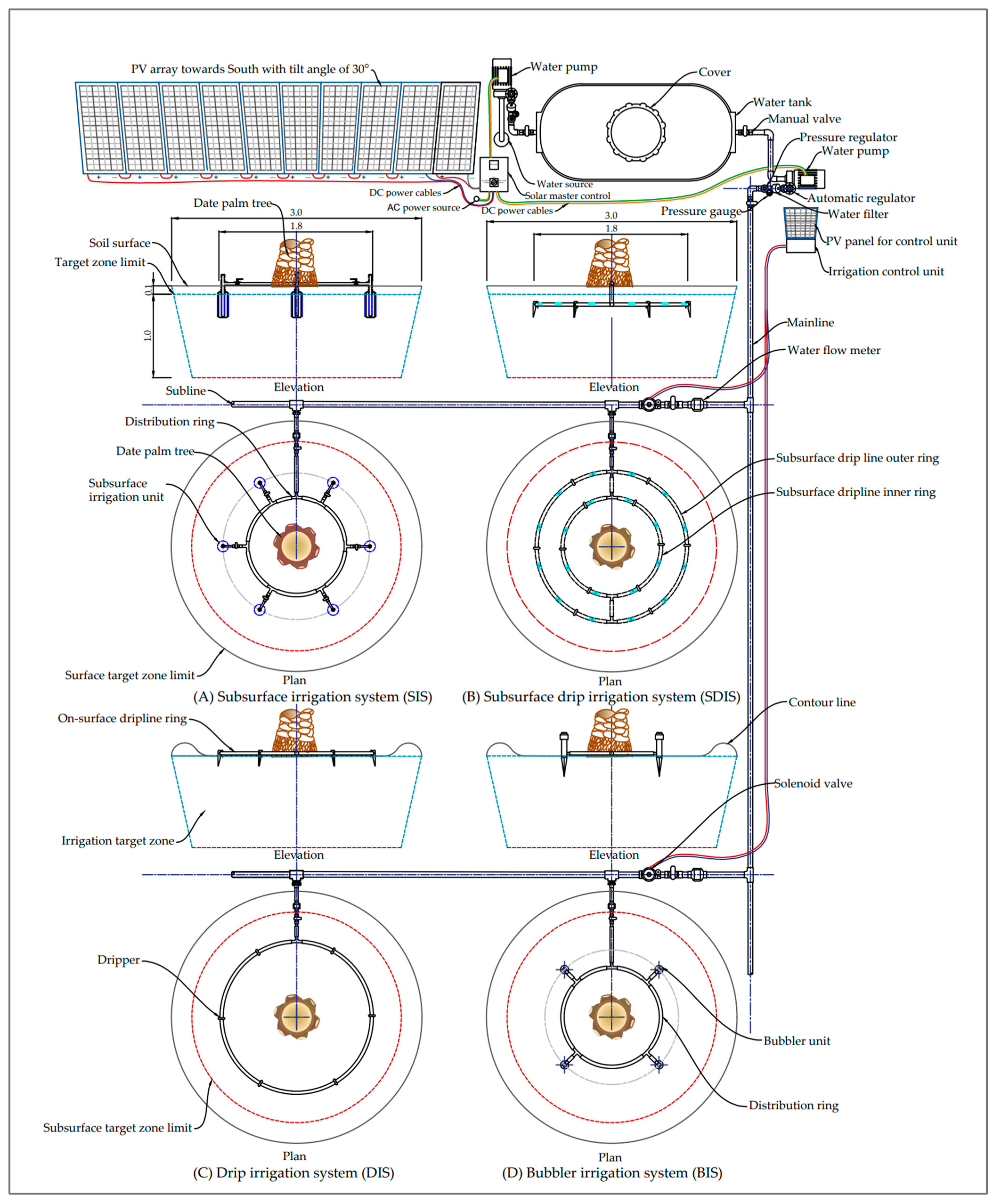
2.2.2. Irrigation Systems

One solar-powered water pumping system was used for these irrigation systems. The water pumping system consisted of a solar-powered irrigation control unit, a water source, two water pumps, pressure regulators, water solenoid valves, manual valves, a pressure gauge, and water flow meters.
The solar-powered irrigation control unit included four digital programable timers, electronic circuits, and power sources for the valves and timers (Figure 2b). Four digital programable timers were used to regulate the water pumping in the irrigation network for each irrigation system separately. The PV system of the irrigation control unit consisted of a 20 W solar panel, battery (12 V, 30 Ah), and solar charging controller.
Figure 1 compares the distribution of irrigation units around the palm tree for SIS (Figure 1A), SDIS (Figure 1B), DIS (Figure 1C), and BIS (Figure 1D). The following is a brief description of the micro irrigation systems used:
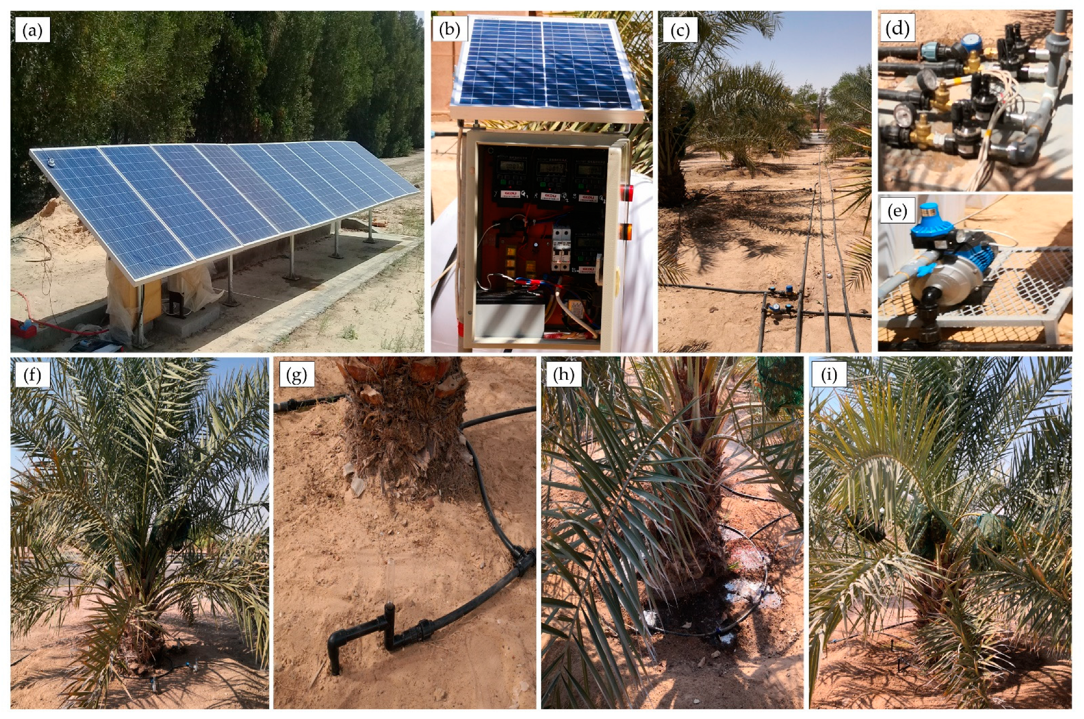
  • SIS: Six subsurface irrigation units were used for each date palm tree in this system (Figure 2f). The subsurface irrigation units were connected to the distribution ring, and the ring was connected to the subline. The subsurface irrigation unit consisted of two perforated pipes with light volcanic gravels (0.4–0.8 cm in diameter) between them. The outer diameter of the subsurface irrigation unit was 12.5 cm, and its length was 35 cm. The outer pipe’s surface is slotted with a slot width of 0.2 cm, a length of 4.0 cm, and a tilt angle of 30°. The inner pipe length is 35 cm with a diameter of 2.5 cm and is perforated in a spiral shape with a 0.3 cm hole diameter. The subsurface irrigation unit’s water flow rate was approximately 0.030 m3/h at a pressure of 300 kPa.
  • SDIS: A subsurface dripline with a diameter of 1.6 cm (Rain Bird Corporation, Tucson, AZ, USA) included subsurface pressure-compensating emitters used in this system (Figure 2g). The distance between two pressure-compensating emitters was 0.457 m. Two lateral rings of this subsurface dripline were installed around the date palm tree. The diameters of the inner and outer lateral dripline rings were 1.2 m and 1.84 m, respectively. Accordingly, twenty pressure-compensating emitters were used for each date palm tree. The flow rate of the pressure-compensating emitters was approximately 0.010 m3/h at a pressure of 380 kPa.
  • DIS: Six pressure-compensating drippers with a flow rate of approximately 0.03 m3/h at 300 kPa were distributed around the date palm tree in this system (Figure 2h). The dripper was installed on a lateral ring (1.6 cm in diameter) around date palm trees with a diameter of 1.80 m.
  • BIS: Four adjustable low-pressure bubblers with flow rates ranging from 0 to 0.120 m3/h were used in this system for each date palm tree (Figure 2i). The bubbler flow rate of 0.045 m3/h was adjusted at the pressure of 200 kPa. The bubbler heads were installed on a wedge and inserted into the ground around the date palm tree.

2.3. Experimental Design and Measurements

The experiment involved four solar-powered micro irrigation systems (SIS, SDIS, DIS, and BIS) with six deficit irrigation level treatments as a different percentage of available water (AW). The experiment was a factorial randomized block design (factorial RBD) with three replicates. Factor one was the four irrigation systems; factor two was the six irrigation levels; and factor three was the date palm age or years of experiment. Therefore, 72 date palm trees were used in this experiment for five successive years from 2018 to 2022 (date palm age was from 14 to 18 years).
Based on the evaluation of irrigation systems, we selected the data of irrigation water amount that presented significant optimum water use efficiency (WUE) and optimum date palm tree yield to develop the ML models for prediction of the optimum irrigation water and PV energy requirements for each micro irrigation system.
The measurements in this study included the meteorological variables, irrigation water requirements at the four deficit irrigation treatments, the actual amount of irrigation water used for each irrigation system, the amount of electrical energy consumed for each irrigation system, date palm yield, and water use efficiency. First, the data of meteorological variables, plant age, and actual water and energy requirements for date palm irrigation for four successive years from 2018 to 2021 were used to train and test four ML-based prediction models for predicting the irrigation water and energy requirements. Then, the data obtained from the fifth season (2022) were used to validate the performance of the best developed model by comparing the observed values with the predicted values. The measurements in the current study can be summarized as follows:
  • Meteorological variables: A cloud-based IoT platform was used for meteorological variables’ data collection. The IoT platform included several components, i.e., the sensors, controller, source of internet, cloud platform (ThingSpeak cloud platform), and laptop. These components were efficiently connected and seamlessly worked to realize the meteorological variables’ data collection.
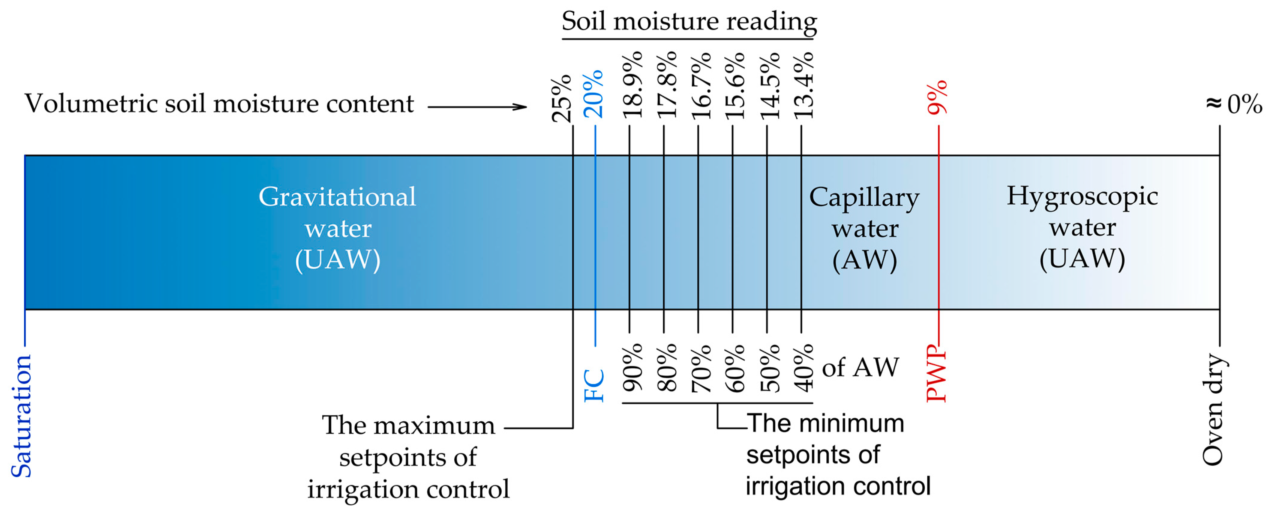
  • Irrigation water requirements: The amount of irrigation water requirements (IWR) was expressed per date palm tree. The IWR was controlled based on the volumetric soil water content (VSWC) using a soil moisture sensor-based control system. The sensor-based irrigation scheduling (SBIS) method was used for the irrigation schedule in this experiment using a soil moisture sensor-based control system designed and manufactured by the first author of the current study [9]. The minimum setpoints were adjusted at different VSWC as a percent of available water (AW) content (40, 50, 60, 70, 80, and 90% of AW), as shown in Figure 3. The maximum setpoints were adjusted at 25% VSWC for all irrigation systems. Three VSWC sensors (VH400Vegetronix, Inc., Riverton, Salt Lake County, UT, USA) were used for each treatment. Each sensor is installed between two irrigation units at a distance of 1 m from the palm tree’s trunk, with a depth of 25 cm.
  • Irrigation water applied: Multi-jet water flow meters (model: LXSG-15E-50E, Ningbo Yonggang Instrument Co., Ltd., Cixi, Ningbo, China) made from copper with a nominal diameter of 20 m were used to calculate the actual amount of irrigation water applied. The flow meters were made of copper with total dimensions of approximately 1.9 × 9.9 × 1.6 cm.
  • The reduction factor: The reduction coefficient (Kr) for each irrigation system was estimated using the following formula:
K r = I W R × 1000 E T c × A i
where Kr is a reduction factor of ETc for achieving the optimum WUE or optimum yield; IWR is the irrigation water requirement applied based on the sensor-based irrigation scheduling (m3/palm/day); ETc is the crop evapotranspiration in the study area (mm/day); Ai is the target irrigation area of each date palm tree. The target irrigation area was equal to 90% of the actual shaded area of the date palm; Ai was determined according to the light intercepted fraction by the canopy.
The ETc was determined according to the following formula:
E T c = K c × E T o
where Kc is the crop factor for the date palm tree ((Kc ranged from 0.8 to 1.0)) [5,33], and ETo is the reference evapotranspiration (mm/day). The ETo was determined according to the Penman–Monteith equation [34].
  • Electrical energy consumed: The amount of electrical energy consumed for each irrigation system was measured using digital energy meters (D69-2049, Yueqing Winston Electric Co., Ltd., Wenzhou, China). These digital energy meters are multi-function meters, which simultaneously display the measured AC voltage (80–300 VAC), AC (0–100 A), active power (0–10000 W), and cumulative energy consumption (0–10000 kWh).
  • Yield and water use efficiency: The yield of the palm tree was predicted by weighing the ripe date fruits immediately after harvesting using a digital balance. The water use efficiency was predicted based on the yield and the cumulative irrigation water applied using the following equation:
W U E = D P Y A I W
where WUE is water use efficiency (kg/m3); DPY is the date palm yield (kg); and AIW is the applied irrigation water (m3).

2.4. Machine-Learning Algorithms

In this study, we developed and evaluated four common ML algorithms widely used to automate the decision making of irrigation systems’ management [7]. In order to reach a fair evaluation, we utilized 60%, 20%, and 20% of the overall dataset in training, testing, and validating, respectively, the ML methods. The following subsections briefly show the ML algorithms, which are developed and utilized in this study.

2.4.1. Linear Regression

Linear regression examines the relationship between two quantitative variables, namely dependent variables (goal) and independent variables (predictor). In practice, it comes in two variants. The first is a simple linear regression where we have one independent variable and one dependent variable. The second is a multi-linear regression where there is more than one independent variable. The multi-linear regression where there is more than one independent variable was used in this study, as shown in the following equation:
y i ^ = B 0 + B 1 x i 1 + B 2 x i 2 +     B n x i n
where y i ^ is the predicted value (output), the Bs are the regression model parameters, and the xis are the input variables.
In this study, the xis represent the meteorological variables and date palm age, whereas the output y i ^ represents the irrigation water required and the solar PV energy, which is required for water pumping and controlling each irrigation system. The values of the Bs started at random and were then adjusted during the learning phase.

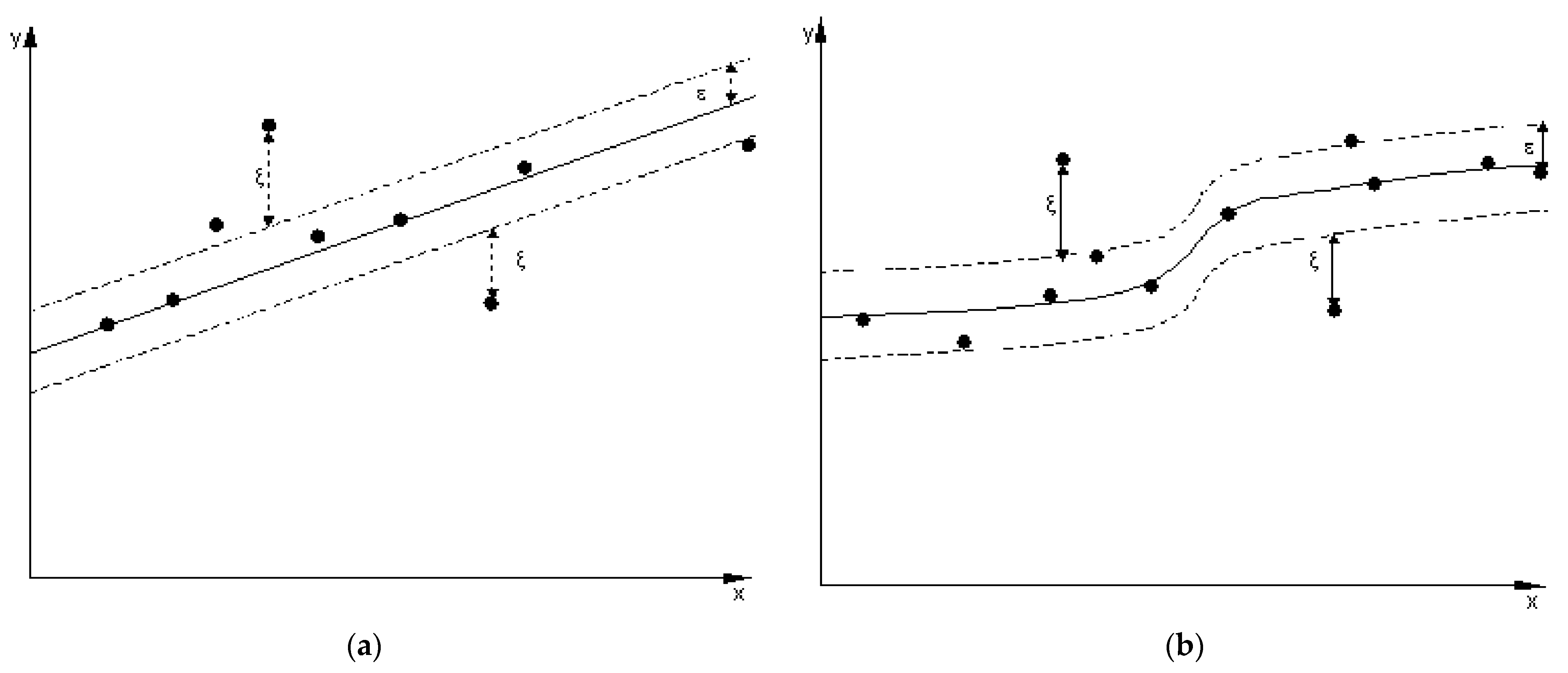
2.4.2. Support Vector Machine

The support vector machine (SVM) is based on two elements of the statistical learning theory, namely the decision boundary and the decision plane. SVM uses a linear function to establish a nonlinear decision boundary across a nonlinear mapping of the input vector x into a high-dimensional feature space. In practice, it uses a linear function to establish a nonlinear decision boundary across a nonlinear mapping of the input vectors x into a high-dimensional feature space. The decision plane can be defined as a plane that separates a set of varied objects [31]. When SVM is applied to a regression problem, it takes the name of support vector regression (SVR) [24]. Similar to the SVM approach, there is motivation to optimize the generalization bounds adopted for SVR. Namely, SVR relies on identifying the loss function by excluding the expected errors, which may exist within a specific distance from the ground values. As shown in Figure 4a, this loss function embeds a uni-dimensional linear regression function with an epsilon-insensitive band; therefore, it is called the epsilon-insensitive loss function.
The goal of SVR is to find a function f x = w T x + b , which deviates no more than ξ from the target values yi for all training data [31]. For linearly separable data, the corresponding quadratic optimization problem is given as
M i n i m i z e 1 2 w T w   s . t . y i w T x i + b 1 ; i = 1,2 ,   ,   N
where w is the weight vector, the xis are the input features (or the weather conditions), and b is the bias. The SVM can deal with nonlinear regression cases, as shown in Figure 4b. For the nonlinearly separable data, the corresponding optimization problem can be given as
M i n i m i z e 1 2 w T w + C i = 1 N ζ   s . t . y i w T x i + b 1 ζ ; i = 1,2 ,   ,   N , ζ 1
where C is a constant usually used to control the error. For the experiments of this study, we considered C = 100, ξ = 0.1, and 0.01 for the irrigation water requirements and the solar PV energy requirements, respectively. For the kernel function of SVR, we used the Gaussian RBF kernel function with γ (Gamma) = 0.1 and 0.01, respectively. Gamma in SVR is a hyperparameter, which decides how much binding we want in a decision boundary.

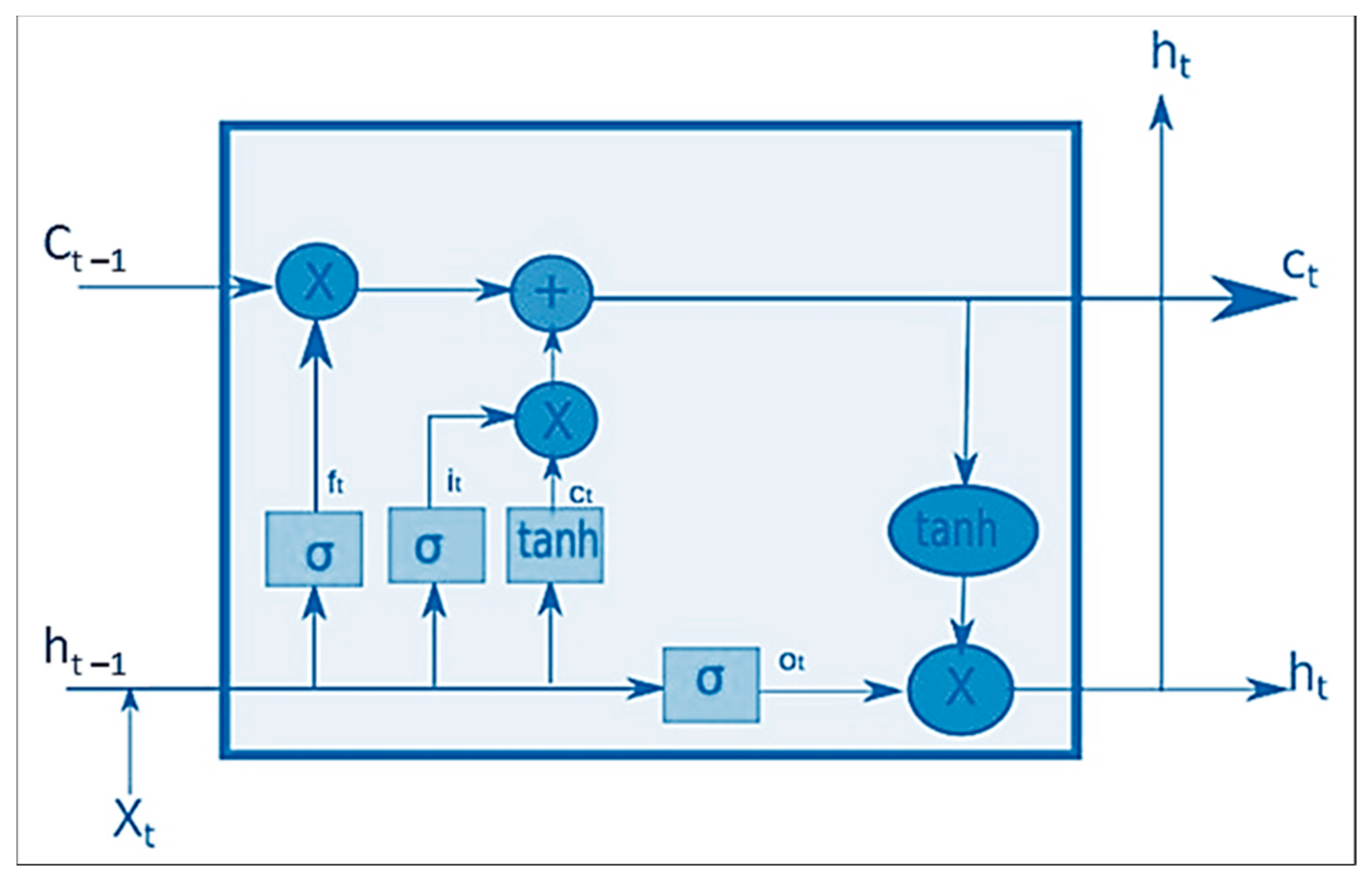
2.4.3. Long Short-Term Memory

Long short-term memory (LSTM) is a recurrent neural network method capable of treating sequential (or time series) data. This is because LSTM contains memory blocks that replace the summation unit in each neuron of other neural network models. The standard LSTM model is composed of one hidden layer followed by a feed-forward output layer. Each layer contains several cells where the information is stored; Figure 5 shows the internal structure of one cell.
As depicted in Figure 5, the LSTM memory cell consists of three gates built upon a sigmoidal neural network, where each gate has a different function [27]. The three gates are the input gate, the forget gate, and the output gate. In detail, the input gate controls whether to enter the input data into the cell state. The forget gate decides whether to erase data from the cell state or not. Lastly, the output gate decides which data to pass as the output hidden state. The following equations represent the function of each gate.
( i t = σ W x i X t + W h i h t 1 + b i
f t = σ W x f X t + W h f h t 1 + b f
o t = σ W x o X t + W h o h t 1 + b o
c t = f t c t 1 + i t t a n h W x c X t + W h c h t 1 + b c
h t = o t t a n h c t
For simplicity, this could be represented in one form as follows:
h t , c t = L S T M x t , h t 1 , c t 1
where it, ft, and ot are the LSTM gating for the cell state to input, forget, and output information, respectively. ht and ct are the hidden state vector and the cell memory state vector, respectively. Xt is the input vector, and σ is the sigmoid activation function. The W’s are linear transformation matrices whose parameters need to be learned for each gate and cell memory; the bs are the corresponding bias vector [35].
In this study, we built the structure of LSTM similar to the model described in our previous paper [35]. Namely, the LSTM includes one input layer, two hidden layers with twelve and six neurons, respectively, and one output layer with two neurons, one for each output. The number of epochs was 250, such that the batch size was 150. The initial learning rate of the model was 0.001 with a suitable decay rate to slow down the training after several epochs.

2.4.4. Gradient Boosting Machine

Gradient boosting (GBoost) machine is a decision-tree-based ensemble algorithm that combines many weak learners, based on the gradient direction of the loss function, to create one stronger learner. GBoost learns the decision trees, in parallel, by fitting the negative gradients in each iteration. To learn the decision tree, GBoost finds the best split points, which takes a long time, making GBoost inapplicable in large-scale problems [36]. The eXtreme gradient boosting (XGBoost) algorithm is an efficient scalable end-to-end implementation of GBoost, even with billions of examples, using far fewer resources than existing systems [37].
As an ensemble learning algorithm, XGBoost works by establishing many independent learners (or classifiers) through random subsamples of the training samples using the bootstrap aggregation mechanism. This subsampling process is conducted across many iterations, plus the algorithm adds more iterations sequentially to adjust the weights of the weak learners [38]. The booster parameter sets the type of learner. Usually, this is either a tree or a linear function. In the case of trees, the model will consist of an ensemble of trees. In the case of the linear booster, it will be a weighted sum of linear functions.
In both cases, the XGBoost calculates the predicted value as
y i ^ = k = 1 K f k ( x i )
where fk represents the independent learner (or a regression tree), and fk(xi) is the prediction score given by that learner for the ith sample. Then, the set of functions fk in the regression tree can be learned by minimizing the objective function
O b j = i = 1 n l ( y i , y i ^ ) + k = 1 K Ω ( f k )
where l is the loss function during training, and Ω is a term for penalizing the model complexity to avoid model overfitting. It is known that the loss function calculates the difference between the predicted value y ^ and the actual value yi [38].
In this study, we selected the objective function as <logistic>, with a linear booster <gblinear> for simplicity.

2.5. Performance Evaluation of the ML Models

Three different performance metrics were used in this study to evaluate each developed ML model’s performance and calculate its forecasting error for each irrigation system. Empirically, the forecasting error is defined as the difference in values between the actual (or observed) values and the predicted values given by the model. This can be mathematically written as
e t = | y t ^ y t |
where et is the forecasting error, y t ^ is the predicted value, and yt is the actual value, all at the same period t.
Generally, forecasting errors can be divided into two kinds of errors, namely residual and prediction errors. The residual errors are calculated using the training dataset, while the prediction errors are calculated using the testing and validation datasets. In this study, we mainly concentrated on calculating the prediction errors using the testing and validating datasets because they are more realistic. Two kinds of prediction errors are employed in this study:
  • Scale-dependent errors. In this kind of error, the forecast errors are on the same scale as the data themselves. The most commonly used scale-dependent errors are root mean square error (RMSE) and the mean absolute error (MAE) [39]. RMSE calculates the square root of the mean of the squares of all errors of all values. In other words, it measures the variance of the residuals. Contrarily, MAE represents the average of the absolute difference between the actual and predicted values in the dataset. In other words, it measures the average of the residuals in the dataset. RMSE is a differentiable function, which makes it easy to perform mathematical operations in comparison to the non-differentiable function, such as MAE. The mathematical formulae of RMSE and MAE can be given as follows:
MSE = mean (et2)
RMSE = M S E
MAE = mean (|et|)
  • Scale-independent errors. In this kind of error, the forecast errors are free scale regardless of the data values being small or large. One of the most commonly used scale-independent errors is the coefficient of determination (usually known as R2). R2 is a performance measure, which provides information about the goodness of fit of a model. In the context of regression, it represents the proportion of the variance in the dependent variable, which is explained by the independent variable [40,41]. Whereas correlation explains the strength of the relationship between an independent and dependent variable, R2 explains to what extent the variance of one variable explains the variance of the other variable.

2.6. Statistical Analysis and ML Hardware and Software Platforms

The statistical analysis was conducted using analysis of variance (ANOVA) for data of meteorological variables, date palm yield, WUE, and electrical energy consumption using Statistical Analysis Software, IBM SPSS version 26 (SPSS Inc., Chicago, IL, USA). The Tukey test was used to determine the significant differences among the means at p ˂ 0.05.
Design Expert software (DX Version 13, Stat-Ease, Inc., Minneapolis, MN, USA) was used to graph the irrigation experiment data and for optimization of the target parameters and variables.
All ML experiments in this study were conducted on an HP workstation PC, Intel Core™ i7-6700 CPU at 3.40 GHz, 16.00 GB RAM ×64 based processor, equipped with an Ubuntu 16.04 operating system with python 3.7 software environment. The ML approaches were developed using the Keras library with an open-source Tensorflow library in the backend [42].

3. Results and Discussion

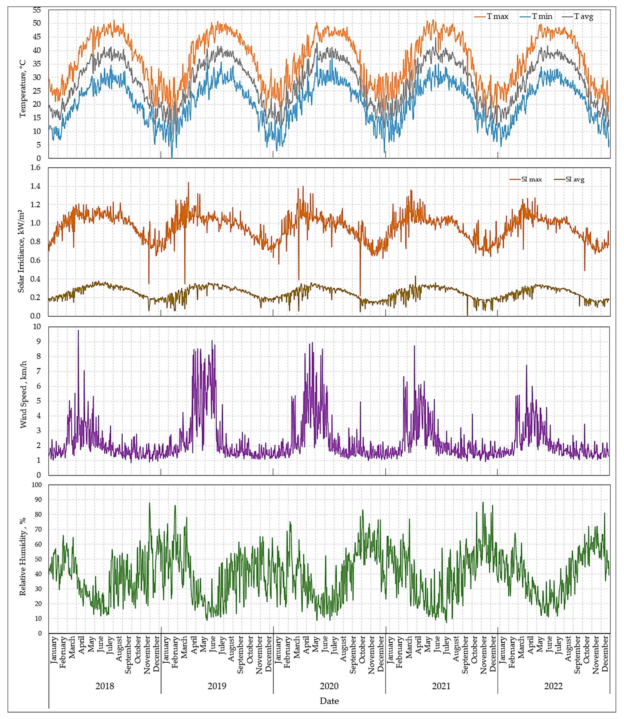
3.1. Meteorological Data Description

The climate of the Al-Ahsa region is characterized by hot dry summers and mild-to-cool winters. Rain is very scarce almost everywhere in this region. In the study area, no rain was received during summer, and a little rain precipitation was received during January and February. Therefore, rain was not considered in this study due to its scarcity.
Table 1 displays the average yearly data of the meteorological variables of sun hour, the minimum, maximum, and average temperature, minimum, maximum, average relative humidity (RH), average wind speed, maximum solar irradiance, average solar irradiance, and solar radiation. The statistical analysis using one-way ANOVA indicated that there were significant differences (p < 0.05) between the years of the experiment regarding the sun hour, temperature, minimum RH, average wind speed, maximum and average solar irradiance, and solar radiation. There was no significant difference for the other variables during the experiment years.
During the experiment years, the coldest month was January with an average daily minimum temperature of 11.62 °C and an average daily maximum temperature of 24.09 °C. The summer season had the hottest months from May to September, and the highest average daily maximum temperature (46.01 °C) was recorded in June, followed by July (45.59 °C). The average daily maximum RH during winter ranged between 73.2 and 63.02%, whereas during summer, it ranged between 46.87 and 29.31%. The average daily minimum RH during winter ranged between 27.1 and 25.2%, whereas during summer, it ranged between 11.12 and 9.51%. The average daily wind speed ranged from 2.71 to 4.29 km. The average daily maximum solar irradiance during winter ranged between 73.2 and 63.02%, whereas during summer, it ranged between 46.87 and 29.31%. The highest average daily solar irradiance was recorded in June (0.978 kW/m2) and the lowest in January (0.662 kW m2). Figure A1 in the Appendix A shows the average daily data of the meteorological variables for five years from 2018 to 2022.

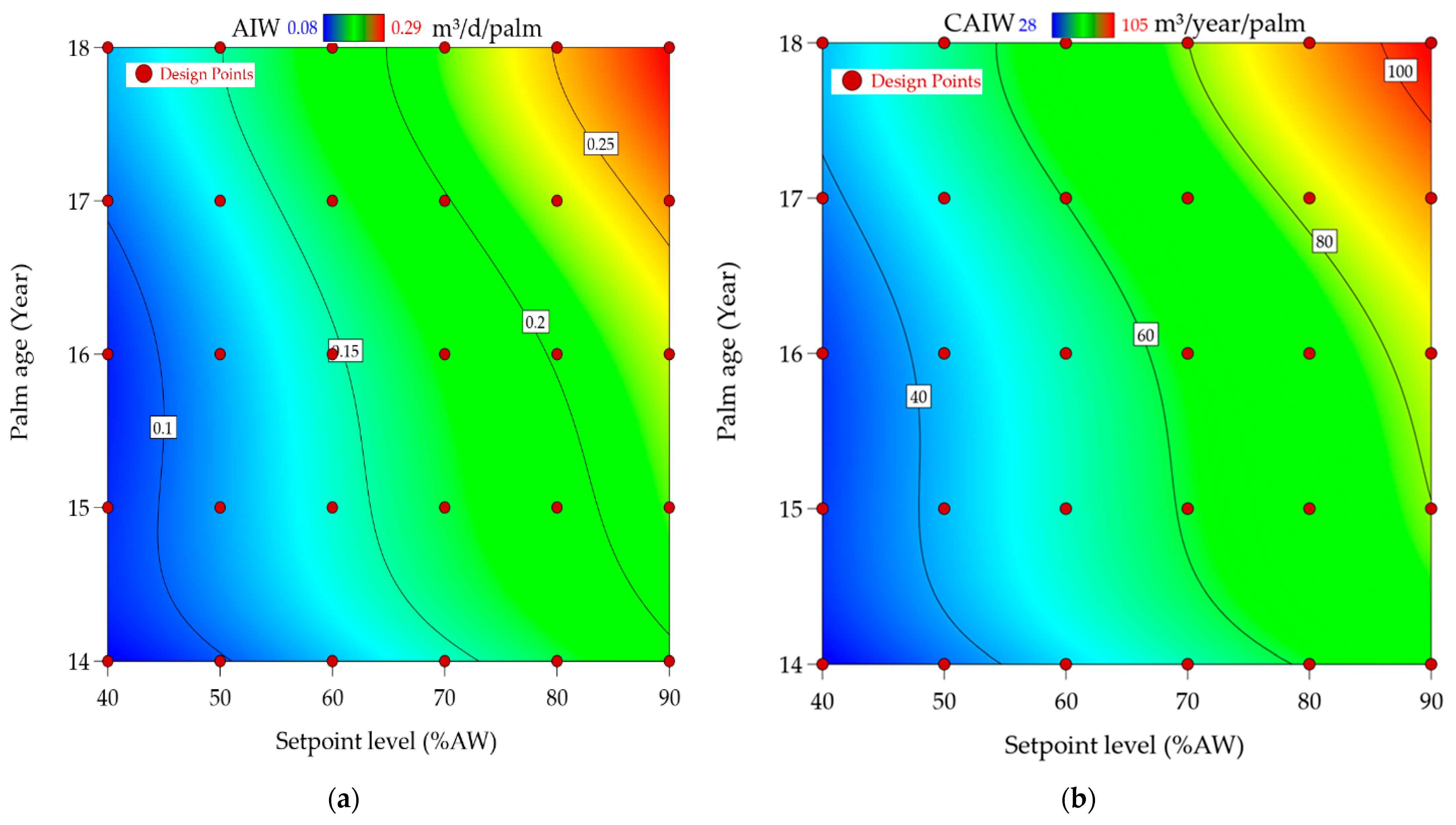
3.2. Irrigation Water Applied

Figure 6 shows the average yearly data of the irrigation water and the cumulative irrigation water applied at irrigation levels. The average yearly irrigation water applied upon adjusting the minimum irrigation control setpoints at 40, 50, 60, 70, 80, and 90% of AW was 0.089 ± 0.03, 0.119 ± 0.03, 0.149 ± 0.05, 0.178 ± 0.06, 0.206 ± 0.07, and 0.232 ± 0.08 m3/day/palm, respectively. The average cumulative irrigation water applied at 40, 50, 60, 70, 80, and 90% AW was 33.43 ± 1.22, 43.89 ± 1.76, 54.32 ± 1.89, 64.32 ± 1.57, 75.65 ± 1.68, and 85.65 ± 1.87 m3/year/palm, respectively. The statistical analysis using two-way ANOVA indicated that there were significant differences (p < 0.01) between the irrigation water applied and the cumulative yearly irrigation under different irrigation level treatments and date palm ages. The interaction effect of the irrigation levels and palm ages on the irrigation water applied (Figure 6a) and the cumulative irrigation water (Figure 6b) was plotted on 3D plots using Design Expert software. This interaction was significant at p < 0.01 regarding the daily irrigation water applied and the yearly cumulative irrigation water. The cumulative irrigation water applied in the irrigation level treatments in the current study was within the irrigation level range mentioned in many previous studies [5,9,43,44,45,46].
Table 2 shows the reference evapotranspiration (ETo), crop evapotranspiration (ETc), target irrigation area, and the reduction coefficient (Kr) when the optimal amount of irrigation water is applied based on soil moisture sensor-based scheduling controller over the five years of the experiment at optimum WUE and date palm yield. The statistical analysis using one-way ANOVA indicated that there were significant differences (p < 0.05) between the years of the experiment regarding the ETo, ETc, target irrigation area, and Kr at optimum WUE and date palm yield.

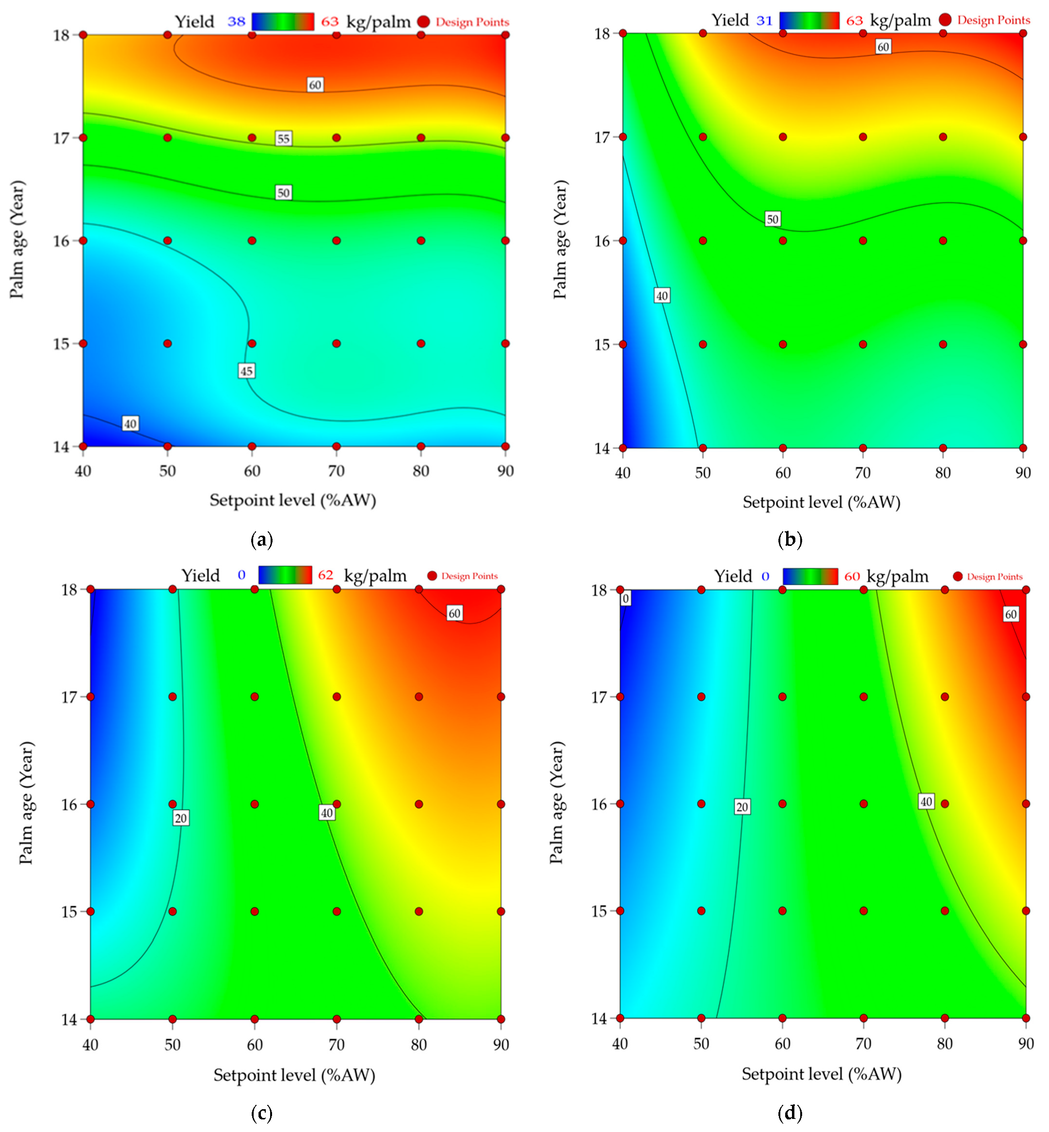
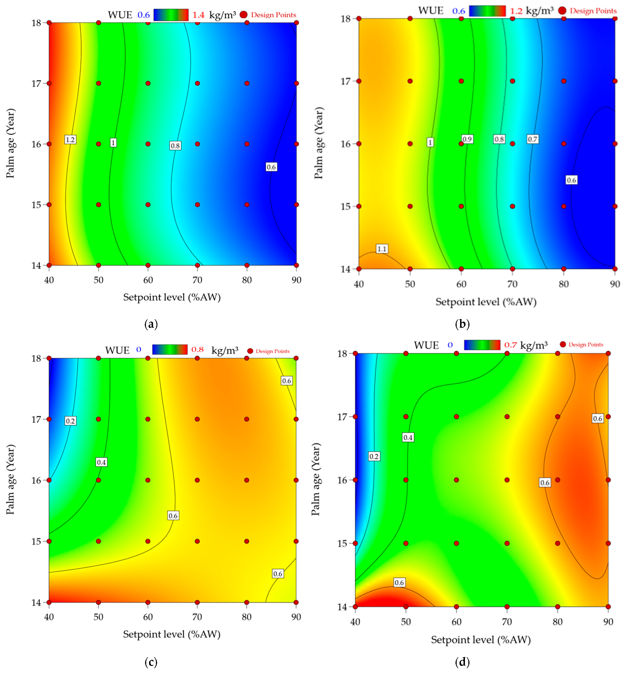
3.3. Yield and Water Use Efficiency

Figure 7 displays the effect of irrigation water levels and palm age on the yield (kg/palm) under the micro irrigation systems used. The interaction effect of the irrigation levels and palm age on palm tree yield under SIS (Figure 7a), SDIS (Figure 7b), DIS (Figure 7c), and BIS (Figure 7d) was plotted on 2D plots using Design Expert software. According to ANOVA, the date palm age, the irrigation system, and the irrigation levels applied had a significant impact (p < 0.05) on the yield of the date palm trees tested.
Figure 7a–d indicated that the date palm trees subjected to SIS and SDIS had the highest yield of 64.31 and 63.28 kg/palm at the irrigation level of 60% AW and 70% AW, followed by DIS (63.2 kg/palm) and BIS (60.19 kg/palm) systems at 80% AW and 90% AW, respectively. The increase in date palm yield at low irrigation levels under SIS and DIS could be due to their high efficiency compared to the surface irrigation systems of DIS and BIS [5,44]. There were no significant differences regarding the palm tree yield when the irrigation level was increased from 60% AW to 90% AW under SIS, from 70% AW to 90% AW under SDIS, and from 80% AW to 90% AW under DIS.
On the other hand, there were significant differences in palm tree yield when the level of irrigation was increased from 40% to 90% AW under BIS. The results indicated that the yield of date palm trees decreased until, in the following years, it stopped at an irrigation level of 40% AW under the two irrigation systems of DIS and BIS. This is because, although the date palm trees can withstand prolonged abiotic stresses, including drought, the long-term water stress leads to a significant reduction in their growth and productivity [47,48,49]. Our results revealed that the increased palm tree yield was related to the subsurface irrigation systems’ optimal availability of soil water, which expedites root growth and enhances the uptake of soil nutrients [6,50,51].
Figure 8 displays the effect of irrigation water levels and palm ages on the water use efficiency (WUE, kg/m3) under the micro irrigation systems used. Figure 8a–d indicated that the date palm trees subjected to SIS had the highest WUE of 1.42 kg/m³ at the irrigation level of 40% AW, followed by SDIS with 1.22 kg/m³ at 50% AW. The highest WUE values were 0.69 and 0.65 kg/m³ at the irrigation level of 70% AW and 80% AW for DIS and BIS, respectively. This is because the use of SIS and SDIS leads to higher yields with lower water consumption; SIS and SDIS also provide more stable irrigation water conditions for optimal root system growth [52]. The highest yield and WUE were reported in date palm cvs.
Although the date palm trees consumed a low amount of irrigation water under SIS and SDIS, this amount was highly efficient for fruit production. This is because most of the irrigation water applied through subsurface irrigation systems is utilized by the palm [53]. SIS and SDIS not only minimize the runoff but also improve soil nutrient uptake and prevent irrigation water loss through evaporation [50,51]. In addition, the drainage losses and evaporation are negligible, and the wetted surface spreads across the entire root zone of the tree [5]. The findings in the current study were similar to those reported in previous studies [5,44].

3.4. Parameters’ Optimization

The optimum WUE and date palm yield were achieved in the current study by applying the optimum irrigation water and solar PV energy requirements. The optimum irrigation water and solar PV energy requirements were determined by optimizing the deficit irrigation water level (% AW) under each micro irrigation system. The objective of this optimization is to achieve the optimum results in the shortest time, conserve water, reduce the photovoltaic energy required, achieve the highest water efficiency and date palm yield, and decrease the irrigation cost. The desirability function approach helps analyze experiments where the multiple responses must be optimized simultaneously [54].
The irrigation level is desired to be as small as possible to decrease the irrigation cost while maintaining date palm yield and WUE. The optimization criterion determined the optimum irrigation level for each irrigation system separately.
In this study, we executed two criteria to optimize the irrigation water and energy requirements for optimum WUE and optimum palm yield. The first criterion was to minimize the irrigation water and energy requirements and maximize the WUE using the minimization of the irrigation level. The second criterion was to minimize the irrigation water and energy requirements and maximize the date palm yield using the minimization of the irrigation level. The two criteria were implemented at date palm ages equal to 14, 15, 16, 17, and 18 years. Table 3 summarizes the constraints imposed by the two criteria for optimizing irrigation water and energy requirements for optimum WUE and date palm yield.
The best solutions for satisfying the optimization criteria are shown in Table 4. In this study, the nearest irrigation level to the irrigation level that was found for satisfying the optimization criteria was used to determine the optimum parameters. Based on these optima, the datasets were prepared to develop the ML prediction models. Table 4 shows the average values of water use efficiency (WUE), date palm yield, irrigation water applied at optimum WUE, irrigation water applied at optimum yield, the electrical energy consumed at optimum WUE, the electrical energy consumed at optimum yield under micro irrigation systems, and date palm ages.

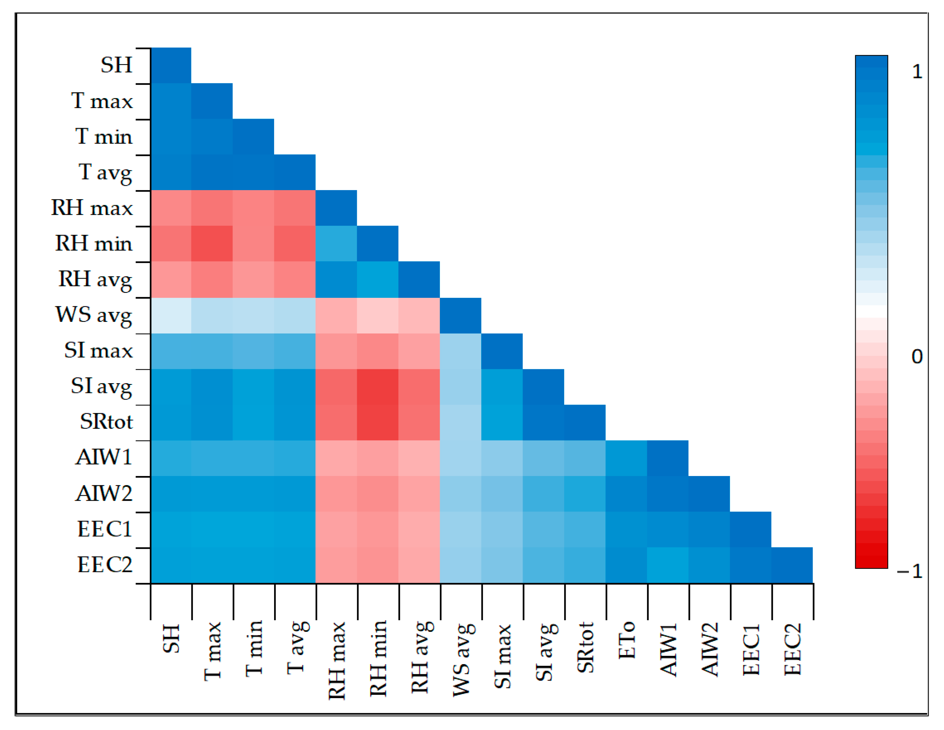
3.5. Variables’ Correlation

Figure 9 shows the correlation among the meteorological variables (sun hour, the minimum, maximum, and average temperature, minimum, maximum, and average RH, average wind speed, maximum solar irradiance, average solar irradiance, and solar radiation), irrigation water applied at optimum water use efficiency and optimum palm yield, and electrical energy consumption at optimum water use efficiency and optimum palm yield. The darker blue color indicates the highly positive correlation between the variables and the parameters. The darker red color indicates the highly negative correlation between the variables and the parameters. The light color indicates that there is no correlation between the variables and the parameters. Figure 9 indicates a positive significant correlation with a correlation coefficient ranging from 0.312 to 0.948 among the sun hour, the maximum temperature, the minimum temperature, the average temperature, average wind speed, maximum solar irradiance, average solar irradiance, and solar radiation, irrigation water applied at optimum water use efficiency and optimum palm yield, and electrical energy consumption at optimum water use efficiency and optimum palm yield. This table also indicates a significant correlation with a correlation coefficient ranging from −0.344 to −0.748 among maximum RH, minimum RH, and average RH, irrigation water applied at optimum water use efficiency and optimum palm yield, and electrical energy consumption at optimum water use efficiency and optimum palm yield. The relation between the meteorological variables and irrigation water and energy requirements obtained in the present study is similar to many previous studies [6,9,13,55].

3.6. Evaluation of the Prediction Models

Based on the results of the irrigation experiments, we selected the data of optimum irrigation water amount that presented significant optimum values of water use efficiency (WUE) (the first option) or optimum yields (the second option) to develop the LR, SVR, LSTM, and XGBoost prediction models for all micro irrigation systems. The deficit irrigation percentages selected based on the optimum WUE and optimum yield were 40% and 60% AW for SIS, 50% and 70% AW for SDIS, 70% and 80% AW for DIS, and 110% and 125% AW for BIS, respectively. These parameters were selected to predict the irrigation water requirements and the electrical energy requirements when the target is to achieve optimum WUE and when the target is to achieve optimum crop yield using solar-powered micro irrigation systems (SIS, SDIS, DIS, and BIS). This will conserve irrigation water and produce optimum yields in arid regions where water scarcity is a significant concern [5,6,9,44]. The evaluation results shown in Table 5 and Table 6 are based on the testing dataset only.
Table 5 shows the comparison among the ML models for predicting the irrigation water and electrical energy requirements based on limited meteorological data, i.e., average temperature, RH, wind speed, solar irradiance, and date palm age, for each irrigation system separately. The evaluation is conducted using three performance metrics, RMSE, MAE, and R2. The lower the value of RMSE and MAE, the higher the accuracy of an ML model. In addition, higher values of R2 that are close to 1.0 are considered optimum. Moreover, Table 6 shows the same comparison among the four ML models but for predicting the irrigation water and electrical energy requirements for each irrigation system separately.

3.7. Analysis of the Prediction Results

It is clear from both Table 5 and Table 6 that both the LSTM and XGBoost models outperformed the other two methods, namely the LR and SVR. In addition, the LSTM surpassed XGBoost in accuracy on the level of all irrigation systems. Therefore, we recommend using the LSTM model to predict irrigation water and electrical energy requirements, whether the target is optimum WUE or optimum crop yield through different solar-powered micro irrigation systems. Even though the experimental results identified LSTM as the best ML model, in the following, we will show the advantages and disadvantages of each model based on our observations during experiments. In order to perform a logic analysis, we will compare the performance of the lower two models together and the performance of the higher two models together.

3.7.1. Comparison between LR and SVR

These two models are similar, since both of them are based on the standard regression concept; however, there are a few differences. The advantage of using the linear regression approach is that limited data are required to train this model. In addition, during our experiments, it showed less computational complexity compared to other models, particularly when predicting the model’s parameters [56]. However, since the irrigation system parameters are highly nonlinear, with complex changing dynamics, linear regression will be suitable for parameters with linear relationships between the predictor and the target [57]. However, in this case, the model may suffer underperformance for a problem, which is nonlinear [7].
Our study here is not unique in using SVR in sustainable farming; rather, it is used widely in this domain. For example, it was used by Goap et al. in Ref [58] to predict soil moisture content using meteorological data and farm sensing data. The prediction choices are made based on the amount of soil moisture and precipitation to save water resources. In the irrigation management domain, Vij et al. [59] used SVR to automate irrigation forecasts by establishing a hyperplane per dimension. In their study, the class labels are chosen, such that the distance between the hyperplanes utilized to identify the best linear classifier is as little as feasible [7]. In our experiments, we noticed that SVR is simple and more powerful than the standard linear regression model. Moreover, we found SVR to be a very time-efficient technique, even though our data and thereby the feature space are highly dimensional. Since our dataset samples are homogenous and mostly noiseless, SVR has a good performance. However, if the data are noisy and include outliers, it is possible that SVR’s performance will degrade drastically [60].

3.7.2. Comparison between XGBoost and LSTM

XGBoost is a tree-based method; however, the LSTM is a neural-network-based model. XGBoost is an ensemble of trees, where each tree is associated with a separate input–output mapping. The final output of the technique represents the weighted sum of the outputs of all the trees (or even linear functions). This process is established in an iterative procedure [61]. In such a sparse environment of trees, XGBoost does not perform well and is very sensitive to outliers because every tree is obliged to fix the defects of predecessor trees. Moreover, it is demonstrated that it is hardly a scalable technique [62].
In contrast, LSTM, or ANN in general, is inspired by the biological neural network in the human brain. ANN simulates neurons and synapses by connecting the artificial neurons. Artificial neurons are typically aggregated into a number of layers, where the connection among layers transmits the input signals from layer to layer. This architecture gives LSTMs more advantages over tree-based methods, such as XGBoost. Recently, a deep architecture for LSTM was developed to model uni-, multi-, and hierarchical time series data in several applications, such as petroleum production [63] and energy consumption [31], to mention a few. In our experiments here, we employed a deep architecture for LSTM, and we found it superior to XGBoost, as shown in Table 5 and Table 6.
The superiority in the performance of LSTM over XGBoost and other models is intuitive and logical in the scope of each method’s characteristics. LR fits a straight line (or a plane), which minimizes the discrepancies between the actual values and the predicted ones [64]. SVR transforms the original feature space into a high-dimensional space. It tries to find a linear mapping in the new space as a sum of nonlinear kernel functions in the original space [65]. For both LR and SVR, the assumption of linearity between variables makes both of them quite prone to overfitting and sensitive to outliers, particularly if the data are complex, as is the case in our dataset, which includes 12 input features. Moreover, such decision boundary-based models, such as the SVR, will not perform well, especially when the dataset has noise and where the target classes may overlap [31].
In addition to the human-brain-like architecture, LSTM has more properties, which make it very suitable for handling sequential data, such as the meteorological data we have here. First, they can remember information for longer periods; therefore, they are capable of handling long-term dependencies among historical data [63]. Second, they can learn high-level representations, which capture the structure of the data, making LSTMs very efficient for modeling complex sequential data. These reasons make LSTMs the most powerful neural network technique, which can achieve forecasting tasks, especially when there is a long-term trend in the data, as in our situation here [66]. Notwithstanding, it is worth mentioning that XGBoost was faster than LSTM in our experiments. Therefore, it is recommended to use XGBoost to achieve feature selection before using LSTM for prediction, which ensures improvement in the overall performance of LSTM [30]. Furthermore, using deep architecture or more hidden layers in LSTM will improve the performance drastically.

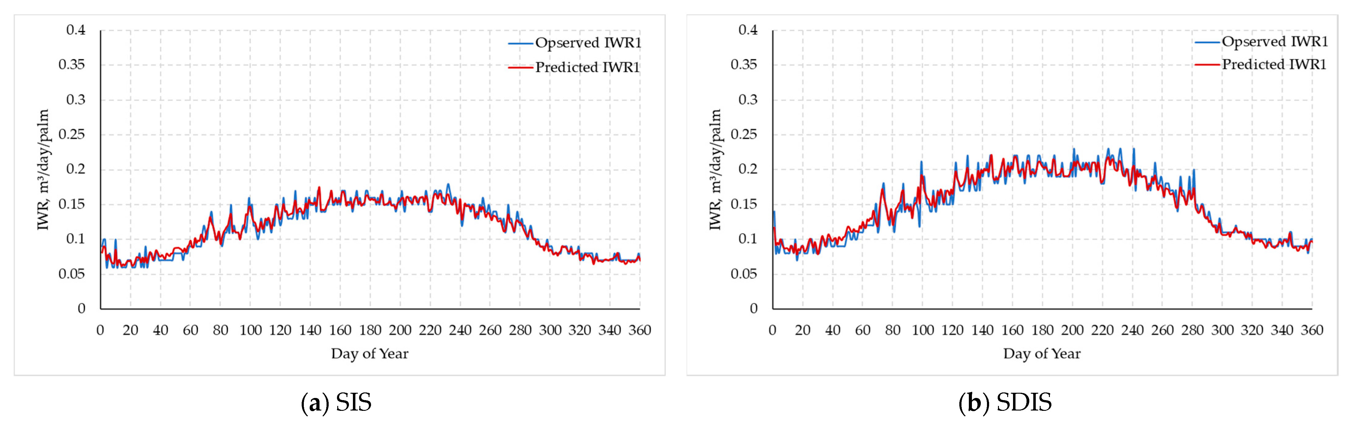
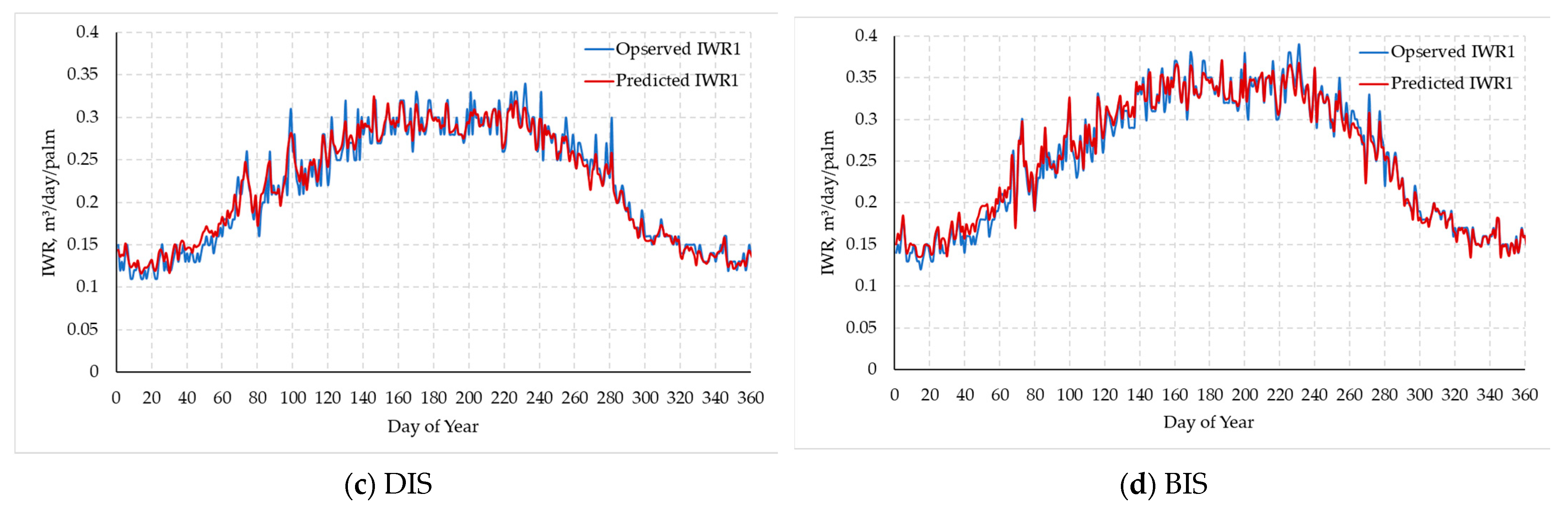
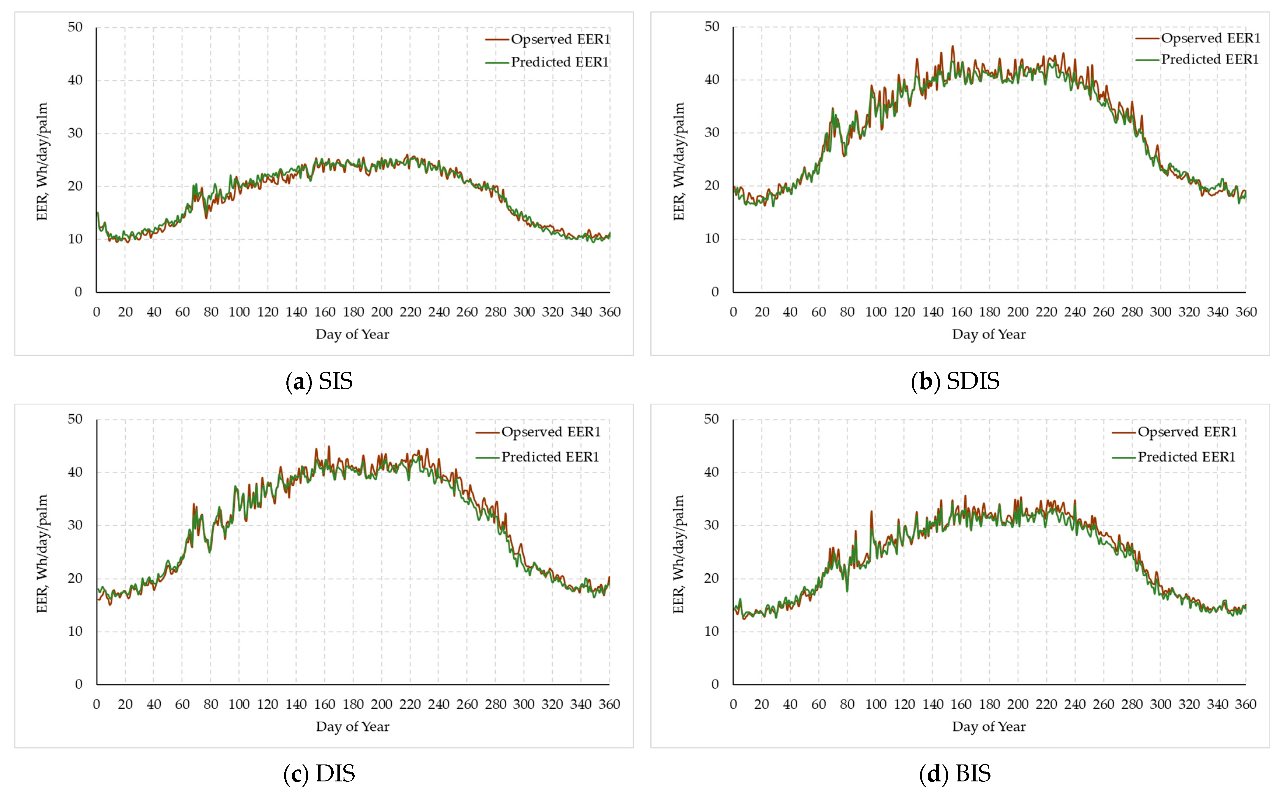
3.8. Validation of the Best ML Model

Based on the performance evaluation of the ML models developed, the LSTM was used to predict the optimum irrigation water requirement based on the limited meteorological data, i.e., average temperature, RH, wind speed, solar irradiance, and date palm age of 18 years, for each micro irrigation system used. Table 7 shows the evaluation of the LSTM model at the validation phase for predicting the irrigation water and energy requirements when the target is to achieve optimal WUS and when the target is to achieve optimal date palm yield. This validation was conducted to ensure that the LSTM model can accurately predict the irrigation water and energy requirements based on the input variables. The evaluation metrics’ values indicated that the LSTM model can efficiently predict the irrigation water and energy requirements, as shown in Table 7.
Figure 10 compares the observed irrigation water applied and the predicted water requirements under the irrigation systems of SIS (Figure 10a), SDIS (Figure 10b), DIS (Figure 10c), and BIS (Figure 10d) using the LSTM prediction model developed based on the limited meteorological data, i.e., average temperature, RH, wind speed, solar irradiance, and date palm age, when the target is to achieve optimum WUE.
Figure 11 compares the observed irrigation water applied and the predicted water requirements under the irrigation systems of SIS (Figure 11a), SDIS (Figure 11b), DIS (Figure 11c), and BIS (Figure 11d) using the LSTM prediction model developed based on the limited meteorological data, i.e., average temperature, RH, wind speed, solar irradiance, and date palm age, when the target is to achieve optimum WUE. The predicted and the observed irrigation water requirements were approximately similar for the majority of the required amounts, where the predicted irrigation water requirements curve was almost identical to the observed irrigation water applied curve under all irrigation systems throughout the year, as shown in Figure 10 and Figure 11.

4. Conclusions

Precision irrigation management is a critical issue for ensuring agricultural sustainability in countries with land and water shortages. In this study, we developed four machine-learning models, namely linear regression, support vector regression, the LSTM neural network, and XGBoost. We employed these models to predict the optimum irrigation water and energy requirements for date palm irrigation. In order to achieve this target, we prepared a dataset, which included limited meteorological data, i.e., average temperature, RH, wind speed, and solar irradiance from 2018 to 2022, and date palm age in these years, actual irrigation water applied, and energy consumed by four surface and subsurface solar-powered micro irrigation systems to achieve the optimum water use efficiency and date palm yield. In order to perform a fair evaluation, we utilized 60%, 20%, and 20% of the overall dataset in training, testing, and validating, respectively, the ML models. The empirical results indicated that the irrigation levels at the minimum irrigation control setpoints of 40% and 60% AW for SIS, 50% and 70% AW for SDIS, 70% and 80% AW for DIS, and 80% and 90% AW for BIS, respectively, achieved optimum WUE and optimum yield. Based on the evaluation of the ML models developed, the best model for predicting the irrigation water and energy requirements for achieving optimum WUE and yield targets was the LSTM, followed by XGBoost. The validation result of the LSTM model showed its ability to predict the water and energy requirements for all irrigation systems with high accuracy based on the limited meteorological variables and date palm tree ages. However, this study was performed in only one cultivar of date palm (Khalas cv.), and the irrigation water and energy requirements of irrigation systems could be different for drought-resistant or other date palm cultivars under different conditions. Therefore, further study is needed to train the ML models to consider other conditions not addressed in this study. Future research will concentrate on more date palm cultivars and irrigation methods to improve the ML models developed, which could also be adapted to predict the irrigation water and energy requirements for other cultivars of agricultural and economic importance or other perennial fruit trees.

Author Contributions

Conceptualization, M.M. and A.S.; methodology, M.M., A.S. and H.H.; engineering design, M.M.; software, M.M., A.S. and H.H.; system manufacturing, M.M.; validation, M.M.; formal analysis, M.M., A.S. and H.H.; investigation, M.M., A.S. and H.H.; data curation, M.M.; writing—original draft preparation, M.M., A.S. and H.H.; writing—review and editing, M.M., A.S. and H.H.; visualization, M.M.; project administration, M.M.; funding acquisition, M.M., A.S. and H.H. All authors have read and agreed to the published version of the manuscript.

Funding

This research was funded by Deputyship for Research & Innovation, Ministry of Education in Saudi Arabia: Grant No. INST089.

Data Availability Statement

The data that support the findings of this study are available from the corresponding author, [M.M.], upon reasonable request.

Acknowledgments

The authors extend their appreciation to the Deputyship for Research & Innovation, Ministry of Education in Saudi Arabia, for funding this research work through project number (INST089).

Conflicts of Interest

All authors declare no conflict of interest.

Nomenclature

AIartificial intelligence
AIWapplied irrigation water
ANNartificial neural network
AWavailable water
BISbubbler irrigation
CAIWcumulative applied irrigation water
DISdrip irrigation
DPAdate palm age
DPYdate palm yield
EEAequal to each age
EECelectrical energy consumption
EERelectrical energy requirements
FCfield capacity
ILirrigation level
Impcurrent at maximum power
Isccurrent at short circuit
IWR
Kr
irrigation water requirements
reduction factor
LRlinear regression
LSTMlong short-term memory
MAEmean absolute error
MLmachine learning
Pmaxmaximum power
PVphotovoltaic system
PWMpulse-width modulation
PWPpermanent wilting point
R2coefficient of determination
RH avgaverage RH
RH maxmaximum RH
RH minminimum RH
RMSEroot mean square error
SBISsensor-based irrigation scheduling
SDISsubsurface drip irrigation
SHsun hour
SI avgaverage solar irradiance
SI maxmaximum solar irradiance
SISsubsurface irrigation system
SPIsolar pumping inverter
SRsolar radiation
SVRsupport vector regression
T avgaverage temperature
T maxmaximum temperature
T minminimum temperature
UAWunavailable water
VFDvariable-frequency
Vmpvoltage at the maximum power
Vocvoltage at open circuit
VSWCvolumetric soil water content
WS avgaverage wind speed
WUEwater use efficiency
XGBoostextreme gradient boosting

Appendix A

Figure A1 shows the average daily data of the meteorological variables, i.e., the maximum temperature, minimum temperature, average temperature, maximum solar irradiance, average solar irradiance, average wind speed, and average RH, for the five years from 1 January to 31 December 2022 in the experimental area using the cloud-based IoT platform.
Figure A1. Average daily values of the maximum temperature (T max), minimum temperature (T min), average temperature (T avg), maximum solar irradiance (IR max), average solar irradiance (IR avg), average wind speed, and average RH for the five years from 1 January to 31 December 2022.
Agronomy 13 01081 g0a1

References

  1. FAO. Water for Sustainable Food and Agriculture Water for Sustainable Food and Agriculture. Rep. Prod. G20 Pres. Ger. 2017, 10–15. Available online: http://www.fao.org/3/i7959e/i7959e.pdf (accessed on 1 February 2023).
  2. Talaviya, T.; Shah, D.; Patel, N.; Yagnik, H.; Shah, M. Implementation of Artificial Intelligence in Agriculture for Optimisation of Irrigation and Application of Pesticides and Herbicides. Artif. Intell. Agric. 2020, 4, 58–73. [Google Scholar] [CrossRef]
  3. Calzadilla, A.; Rehdanz, K.; Tol, R.S.J. Water Scarcity and the Impact of Improved Irrigation Management: A Computable General Equilibrium Analysis. Agric. Econ. 2011, 42, 305–323. [Google Scholar] [CrossRef]
  4. Change, IPCC Climate. Impacts, Adaptation, and Vulnerability: Contribution of Working Group II to the Fifth Assessment Report of the Intergovernmental Panel on Climate Change. Intergov. Panel Clim. Chang. 2014, 1–44. Available online: https://www.cambridge.org/core/books/climate-change-2014-impacts-adaptation-and-vulnerability-part-a-global-and-sectoral-aspects/1BE4ED76F97CF3A75C64487E6274783A (accessed on 1 March 2023).
  5. Ahmed Mohammed, M.E.; Refdan Alhajhoj, M.; Ali-Dinar, H.M.; Munir, M. Impact of a Novel Water-Saving Subsurface Irrigation System on Water Productivity, Photosynthetic Characteristics, Yield, and Fruit Quality of Date Palm under Arid Conditions. Agronomy 2020, 10, 1265. [Google Scholar] [CrossRef]
  6. Mohammed, M.; Sallam, A.; Munir, M.; Ali-Dinar, H. Effects of Deficit Irrigation Scheduling on Water Use, Gas Exchange, Yield, and Fruit Quality of Date Palm. Agronomy 2021, 11, 2256. [Google Scholar] [CrossRef]
  7. Abioye, E.A.; Hensel, O.; Esau, T.J.; Elijah, O.; Abidin, M.S.Z.; Ayobami, A.S.; Yerima, O.; Nasirahmadi, A. Precision Irrigation Management Using Machine Learning and Digital Farming Solutions. AgriEngineering 2022, 4, 70–103. [Google Scholar] [CrossRef]
  8. Sagheer, A.; Mohammed, M.; Riad, K.; Alhajhoj, M. A Cloud-Based IoT Platform for Precision Control of Soilless Greenhouse Cultivation. Sensors 2021, 21, 223. [Google Scholar] [CrossRef]
  9. Mohammed, M.; Riad, K.; Alqahtani, N. Efficient Iot-Based Control for a Smart Subsurface Irrigation System to Enhance Irrigation Management of Date Palm. Sensors 2021, 21, 3942. [Google Scholar] [CrossRef]
  10. Abdelouahhab, Z.; Arias-Jimenez, E.J. Date Palm Cultivation; Food and Agriculture Organization (FAO): Rome, Italy, 1999. [Google Scholar]
  11. Food and Agriculture Organization of the United (FAO); International Center for Advanced Mediterranean Agronomic Studies (CIHEAM). Workshop on “Irrigation of Date Palm and Associated Crops”; Faculty of Agriculture, Damascus University: Damascus, Syrian, 27–30 May 2008; pp. 27–30. ISBN 9789251059975. [Google Scholar]
  12. Wen, Y.; Shang, S.; Yang, J. Optimization of Irrigation Scheduling for Spring Wheat with Mulching and Limited Irrigation Water in an Arid Climate. Agric. Water Manag. 2017, 192, 33–44. [Google Scholar] [CrossRef]
  13. Eltawil, M.A.; Alhashem, H.A.; Alghannam, A.O. Design of a Solar PV Powered Variable Frequency Drive for a Bubbler Irrigation System in Palm Trees Fields. Process Saf. Environ. Prot. 2021, 152, 140–153. [Google Scholar] [CrossRef]
  14. Rehman, S.; Sahin, A.Z. Performance Comparison of Diesel and Solar Photovoltaic Power Systems for Water Pumping in Saudi Arabia. Int. J. Green Energy 2015, 12, 702–713. [Google Scholar] [CrossRef]
  15. Cervera-Gascó, J.; Perea, R.G.; Montero, J.; Moreno, M.A. Prediction Model of Photovoltaic Power in Solar Pumping Systems Based on Artificial Intelligence. Agronomy 2022, 12, 693. [Google Scholar] [CrossRef]
  16. Nam, S.; Kang, S.; Kim, J. Maintaining a Constant Soil Moisture Level Can Enhance the Growth and Phenolic Content of Sweet Basil Better than Fluctuating Irrigation. Agric. Water Manag. 2020, 238, 106203. [Google Scholar] [CrossRef]
  17. Mohammed, M.; El-Shafie, H.; Munir, M. Development and Validation of Innovative Machine Learning Models for Predicting Date Palm Mite Infestation on Fruits. Agronomy 2023, 13, 494. [Google Scholar] [CrossRef]
  18. Mohammed, M.; Riad, K.; Alqahtani, N. Design of a Smart IoT-Based Control System for Remotely Managing Cold Storage Facilities. Sensors 2022, 22, 4680. [Google Scholar] [CrossRef] [PubMed]
  19. Mohammed, M.; Munir, M.; Ghazzawy, H.S. Design and Evaluation of a Smart Ex Vitro Acclimatization System for Tissue Culture Plantlets. Agronomy 2022, 13, 78. [Google Scholar] [CrossRef]
  20. Abioye, E.A.; Abidin, M.S.Z.; Mahmud, M.S.A.; Buyamin, S.; AbdRahman, M.K.I.; Otuoze, A.O.; Ramli, M.S.A.; Ijike, O.D. IoT-Based Monitoring and Data-Driven Modelling of Drip Irrigation System for Mustard Leaf Cultivation Experiment. Inf. Process. Agric. 2020, 8, 270–283. [Google Scholar] [CrossRef]
  21. Yartu, M.; Cambra, C.; Navarro, M.; Rad, C.; Arroyo, Á.; Herrero, Á. Humidity Forecasting in a Potato Plantation Using Time-Series Neural Models. J. Comput. Sci. 2022, 59, 101547. [Google Scholar] [CrossRef]
  22. Chen, A.; Orlov-Levin, V.; Meron, M. Applying High-Resolution Visible-Channel Aerial Imaging of Crop Canopy to Precision Irrigation Management. Agric. Water Manag. 2019, 216, 196–205. [Google Scholar] [CrossRef]
  23. Sapankevych, N.; Sankar, R. Time Series Prediction Using Support Vector Machines: A Survey. IEEE Comput. Intell. Mag. 2009, 4, 24–38. [Google Scholar] [CrossRef]
  24. Vapnik, V.; Golowich, S.E.; Smola, A. Support Vector Method for Function Approximation, Regression Estimation, and Signal Processing. In Proceedings of the Advances in Neural Information Processing Systems NIPS’96, Proceedings of the 9th International Conference on Neural Information Processing Systems; Jordan, M., Petsche, T., Eds.; MIT Press: Cambridge, MA, USA, 1997; pp. 281–287. Available online: https://cir.nii.ac.jp/crid/1572543025363322368 (accessed on 1 March 2023).
  25. Tealab, A. Time Series Forecasting Using Artificial Neural Networks Methodologies: A Systematic Review. Futur. Comput. Inform. J. 2018, 3, 334–340. [Google Scholar] [CrossRef]
  26. Montgomery, D.; Jennings, C.; Kulahci, M. Introduction to Time Series Analysis and Forecasting, 2nd ed.; John Wiley and Sons: Hoboken, NJ, USA, 2015; Volume 2, ISBN 978-1-118-74515-1. [Google Scholar]
  27. Hochreiter, S.; Schmidhuber, J. Long Short-Term Memory. Neural Comput. 1997, 9, 1735–1780. [Google Scholar] [CrossRef] [PubMed]
  28. Jaitly, N.; Senior, A.; Vanhoucke, V.; Nguyen, P.; Sainath, T.; Kingsbury, B.; Hinton, G.; Deng, L.; Yu, D.; Dahl, G.; et al. Deep Neural Networks for Acoustic Modeling in Speech Recognition. IEEE Signal Process. Mag. 2012, 29, 82–97. [Google Scholar]
  29. Sutskever, I. Training Recurrent Neural Networks by Diffusion. Ph.D. Thesis, University of Toronto, Toronto, ON, Canada, 2012. Available online: http://www.cs.utoronto.ca/~ilya/pubs/ilya_sutskever_phd_thesis.pdf (accessed on 1 March 2023).
  30. Vuong, P.H.; Dat, T.T.; Mai, T.K.; Uyen, P.H.; Bao, P.T. Stock-Price Forecasting Based on XGBoost and LSTM. Comput. Syst. Sci. Eng. 2022, 40, 237–246. [Google Scholar] [CrossRef]
  31. Hamdoun, H.; Sagheer, A.; Youness, H. Energy Time Series Forecasting-Analytical and Empirical Assessment of Conventional and Machine Learning Models. J. Intell. Fuzzy Syst. 2021, 40, 12477–12502. [Google Scholar] [CrossRef]
  32. Sagheer, A.; Hamdoun, H.; Youness, H. Deep LSTM-Based Transfer Learning Approach for Coherent Forecasts in Hierarchical Time Series. Sensors 2021, 21, 4379. [Google Scholar] [CrossRef]
  33. AL-Omran, A.; Eid, S.; Alshammari, F. Crop Water Requirements of Date Palm Based on Actual Applied Water and Penman–Monteith Calculations in Saudi Arabia. Appl. Water Sci. 2019, 9, 69. [Google Scholar] [CrossRef] [Green Version]
  34. Clarke, D.; Smith, M.; El-Askari, K. CropWat for Windows; Version 4.2; Southampton University: Southampton, UK, 1998; p. 43. [Google Scholar]
  35. Hochreiter, S.; Schmidhuber, J. Bridging Long Time Lags by Weight Guessing and “Long Short-Term Memory”. In Spatiotemporal Models in Biological and Artificial Systems; Silva, F.L., Principe, J.C., Almeida, L.B., Eds.; IOS Press: Amsterdam, Netherlands, 1996; Volume 37, pp. 65–72. [Google Scholar]
  36. Ke, G.; Meng, Q.; Finley, T.; Wang, T.; Chen, W.; Ma, W.; Ye, Q.; Liu, T.-Y. LightGBM: A Highly Efficient Gradient Boosting Decision Tree. In Proceedings of the 31st Conference on Neural Information Processing Systems (NIPS), Long Beach, CA, USA, 4 December 2017; Curran Associates 57 Morehouse Lane Red Hook: New York, NY, USA, 2017. [Google Scholar]
  37. Chen, T.; Guestrin, C. XGBoost: A Scalable Tree Boosting System. In Proceedings of the ACM SIGKDD International Conference on Knowledge Discovery and Data Mining, San Francisco, CA, USA, 13–17 August 2016; pp. 785–794. [Google Scholar] [CrossRef] [Green Version]
  38. Chen, M.; Liu, Q.; Chen, S.; Liu, Y.; Zhang, C.-H.; Liu, R. XGBoost-Based Algorithm Interpretation and Application on Post-Fault Transient Stability Status Prediction of Power System. IEEE Access 2019, 7, 13149–13158. [Google Scholar] [CrossRef]
  39. Hyndman, R.J.; Koehler, A.B. Another Look at Measures of Forecast Accuracy. Int. J. Forecast. 2006, 22, 679–688. [Google Scholar] [CrossRef] [Green Version]
  40. Piepho, H.P. A Coefficient of Determination (R2) for Generalized Linear Mixed Models. Biom. J. 2019, 61, 860–872. [Google Scholar] [CrossRef]
  41. Chicco, D.; Warrens, M.J.; Jurman, G. The Coefficient of Determination R-Squared Is More Informative than SMAPE, MAE, MAPE, MSE and RMSE in Regression Analysis Evaluation. PeerJ Comput. Sci. 2021, 7, e623. [Google Scholar] [CrossRef]
  42. Abadi, M.; Barham, P.; Chen, J.; Chen, Z.; Davis, A.; Dean, J.; Devin, M.; Ghemawat, S.; Irving, G.; Isard, M.; et al. Tensor-Flow: Large-Scale Machine Learning on Heterogeneous Systems. In Proceedings of the 12th USENIX Symposium on Operating Systems Design and Implementation (OSDI ’16), Savannah, GA, USA, 2–4 November 2016; USENIX Association: Savannah, GA, USA, 2015; Volume 81, pp. 265–283. [Google Scholar]
  43. Adil, M.; Samia, H.; Sakher, M.; El Hafed, K.; Naima, K.; Kawther, L.; Tidjani, B.; Abdesselam, B.; Bensalah, L.M.; Yamina, K.; et al. Date Palm (Phoenix dactylifera L.) Irrigation Water Requirements as Affected by Salinity in Oued Righ Conditions, North Eastern Sahara, Algeria. Asian J. Crop Sci. 2015, 7, 174–185. [Google Scholar] [CrossRef] [Green Version]
  44. Alnaim, M.A.; Mohamed, M.S.; Mohammed, M.; Munir, M. Effects of Automated Irrigation Systems and Water Regimes on Soil Properties, Water Productivity, Yield and Fruit Quality of Date Palm. Agriculture 2022, 12, 343. [Google Scholar] [CrossRef]
  45. Ismail, S.M.; Al-Qurashi, A.D.; Awad, M.A. Optimization of Irrigation Water Use, Yield, and Quality of “Nabbut-Saif” Date Palm under Dry Land Conditions. Irrig. Drain. 2014, 63, 29–37. [Google Scholar] [CrossRef]
  46. Ghazzawy, H.S.; Alqahtani, N.; Munir, M.; Alghanim, N.S.; Mohammed, M. Combined Impact of Irrigation, Potassium Fertilizer, and Thinning Treatments on Yield, Skin Separation, and Physicochemical Properties of Date Palm Fruits. Plants 2023, 12, 1003. [Google Scholar] [CrossRef] [PubMed]
  47. Tripler, E.; Shani, U.; Mualem, Y.; Ben-Gal, A. Long-Term Growth, Water Consumption and Yield of Date Palm as a Function of Salinity. Agric. Water Manag. 2011, 99, 128–134. [Google Scholar] [CrossRef]
  48. Shareef, H.J.; Alhamd, A.S.; Naqvi, S.A.; Eissa, M.A. Adapting Date Palm Offshoots to Long-Term Irrigation Using Groundwater in Sandy Soil. Folia Oecologica 2021, 48, 55–62. [Google Scholar] [CrossRef]
  49. Ali-Dinar, H.; Mohammed, M.; Munir, M. Effects of Pollination Interventions, Plant Age and Source on Hormonal Patterns and Fruit Set of Date Palm (Phoenix Dactylifera L.). Horticulturae 2021, 7, 427. [Google Scholar] [CrossRef]
  50. Bainbridge, D.A. Deep Pipe Irrigation. The Overstory# 175; Permanent Agriculture Resources: Holualoa, HI, USA, 2006; Volume 175, p. 6. [Google Scholar]
  51. Manzoor Alam, S. Nutrient Uptake by Plants Under Stress Conditions. Handb. Plant Crop Stress 1999, 2, 285–313. [Google Scholar] [CrossRef]
  52. Sinobas, L.R.; Rodríguez, M.G.; Lee, T.S. A Review of Subsurface Drip Irrigation and Its Management. In Water Quality, Soil and Managing Irrigation of Crops; InTech: Rijeka, Croatia, 2012; pp. 171–194. [Google Scholar]
  53. Albasha, R.; Mailhol, J.C.; Cheviron, B. Compensatory Uptake Functions in Empirical Macroscopic Root Water Uptake Models—Experimental and Numerical Analysis. Agric. Water Manag. 2015, 155, 22–39. [Google Scholar] [CrossRef] [Green Version]
  54. Mohammed, M.; Munir, M.; Aljabr, A. Prediction of Date Fruit Quality Attributes during Cold Storage Based on Their Electrical Properties Using Artificial Neural Networks Models. Foods 2022, 11, 1666. [Google Scholar] [CrossRef] [PubMed]
  55. Allen, R.G.; Pereira, L.S.; Pereira, L.S.; Raes, D.; Smith, M. Crop Evapotranspiration-Guidelines for Computing Crop Water Requirements-FAO Irrigation and Drainage Paper 56; Fao: Rome, Italy, 1998; Volume 300, p. D05109. [Google Scholar]
  56. Torres-Sanchez, R.; Navarro-Hellin, H.; Guillamon-Frutos, A.; San-Segundo, R.; Ruiz-Abellón, M.C.; Domingo-Miguel, R. A Decision Support System for Irrigation Management: Analysis and Implementation of Different Learning Techniques. Water 2020, 12, 548. [Google Scholar] [CrossRef] [Green Version]
  57. Kumar, A.; Surendra, A.; Mohan, H.; Muthu Valliappan, K.; Kirthika, N. Internet of Things Based Smart Irrigation Using Regression Algorithm. In Proceedings of the 2017 International Conference on Intelligent Computing, Instrumentation and Control Technologies, ICICICT, Kerala, India, 6–7 July 2017; Volume 2018-Janua, pp. 1652–1657. [Google Scholar]
  58. Goap, A.; Sharma, D.; Shukla, A.K.; Rama Krishna, C. An IoT Based Smart Irrigation Management System Using Machine Learning and Open Source Technologies. Comput. Electron. Agric. 2018, 155, 41–49. [Google Scholar] [CrossRef]
  59. Vij, A.; Vijendra, S.; Jain, A.; Bajaj, S.; Bassi, A.; Sharma, A. IoT and Machine Learning Approaches for Automation of Farm Irrigation System. Procedia Comput. Sci. 2020, 167, 1250–1257. [Google Scholar] [CrossRef]
  60. Yu, X.; Wang, Y.; Wu, L.; Chen, G.; Wang, L.; Qin, H. Comparison of Support Vector Regression and Extreme Gradient Boosting for Decomposition-Based Data-Driven 10-Day Streamflow Forecasting. J. Hydrol. 2020, 582, 124293. [Google Scholar] [CrossRef]
  61. Zhang, L.; Bian, W.; Qu, W.; Tuo, L.; Wang, Y. Time Series Forecast of Sales Volume Based on XGBoost. J. Phys. Conf. Ser. 2021, 1873, 012067. [Google Scholar] [CrossRef]
  62. Bhakta, A.; Kim, Y.; Cole, P. Comparing Machine Learning-Centered Approaches for Forecasting Language Patterns During Frustration in Early Childhood. arXiv 2021, arXiv:2110.15778. [Google Scholar] [CrossRef]
  63. Sagheer, A.; Kotb, M. Time Series Forecasting of Petroleum Production Using Deep LSTM Recurrent Networks. Neurocomputing 2019, 323, 203–213. [Google Scholar] [CrossRef]
  64. Mutombo, N.M.-A.; Numbi, B.P. Development of a Linear Regression Model Based on the Most Influential Predictors for a Research Office Cooling Load. Energies 2022, 15, 5097. [Google Scholar] [CrossRef]
  65. Cortez, P.; Donate, J.P. Evolutionary Support Vector Machines for Time Series Forecasting. In Artificial Neural Networks and Machine Learning–ICANN 2012, Proceedings of the 22nd International Conference on Artificial Neural Networks, Lausanne, Switzerland, 11–14 September 2012; Springer: Berlin/Heidelberg, Germany, 2012; Volume 7553, pp. 523–530. [Google Scholar] [CrossRef] [Green Version]
  66. Sagheer, A.; Kotb, M. Unsupervised Pre-Training of a Deep LSTM-Based Stacked Autoencoder for Multivariate Time Series Forecasting Problems. Sci. Rep. 2019, 9, 19038. [Google Scholar] [CrossRef] [PubMed] [Green Version]
Figure 1. A schematic diagram of the experimental setup of the four solar-powered micro irrigation systems: (A) subsurface irrigation (SIS), (B) subsurface drip irrigation (SDIS), (C) drip irrigation (DIS), and (D) bubbler irrigation (BIS) connected with the solar PV system.
Agronomy 13 01081 g001
Figure 2. Experimental setup of the solar PV and irrigation systems: (a) PV array toward south with a tilt angle of 30°, (b) irrigation control unit with small PV system, (c) irrigation network, (d) solenoid valves and pressure regulators, (e) irrigation water pump with an automatic regulator, (f) subsurface irrigation system (SIS), (g) subsurface drip irrigation system (SDIS), (h) drip irrigation system (DIS), (i) bubbler irrigation system (BIS).
Agronomy 13 01081 g002
Figure 3. Water type, thresholds for soil in the study area, and minimum and maximum irrigation control setpoints. The FC, AW, PWP, and UAW denote field capacity, available water, permanent wilting point, and unavailable water.
Agronomy 13 01081 g003
Figure 4. The epsilon-insensitive band via one-dimensional (a) linear regression function and (b) nonlinear regression function.
Agronomy 13 01081 g004
Figure 5. The internal structure of one LSTM cell.
Agronomy 13 01081 g005
Figure 6. Amount of daily applied irrigation water (AIW) per date palm tree (a) and cumulative yearly applied irrigation water (CAIW) per date palm tree (b) at different minimum irrigation control setpoints (%AW) and date palm ages during the experiment years from 2018 to 2022.
Agronomy 13 01081 g006
Figure 7. Effect of irrigation water levels at the different minimum irrigation control setpoints (%AW) and palm ages (year) on palm tree yield cv. Khalas (kg/palm) under different micro irrigation systems, i.e., (a) subsurface irrigation system, (b) subsurface drip irrigation system, (c) drip irrigation system, and (d) bubbler irrigation system.
Agronomy 13 01081 g007
Figure 8. Effect of irrigation water levels at the different minimum setpoints (%AW) and palm ages (year) on water use efficiency (WUE, kg/palm) under different micro irrigation systems, i.e., (a) subsurface irrigation system, (b) subsurface drip irrigation system, (c) drip irrigation system, and (d) bubbler irrigation system, of date palm cv. Khalas.
Agronomy 13 01081 g008
Figure 9. The correlation among the meteorological variables, irrigation water applied, and electrical energy consumption. SR, T max, T min, T avg, RH max, RH min, RH avg, WS avg, SI max, SI avg, SR, AIW1 and AIW2, and EEC1 and EEC2 refer to sun hour, the maximum temperature, minimum temperature, average temperature, maximum RH, minimum RH, average RH, average wind speed, maximum solar irradiance, average solar irradiance, solar radiation, reference evapotranspiration, crop evapotranspiration, applied irrigation water at optimum water use efficiency and optimum palm yield, and electrical energy consumption at optimum water use efficiency and optimum palm yield, respectively.
Agronomy 13 01081 g009
Figure 10. Observed vs. predicted values of irrigation water requirements (IWR1) for optimum water use efficiency under (a) subsurface irrigation system, (b) subsurface drip irrigation system, (c) drip irrigation system, and (d) bubbler irrigation system.
Agronomy 13 01081 g010aAgronomy 13 01081 g010b
Figure 11. Observed vs. predicted values of electrical energy requirements (EER1) for optimum energy use under (a) subsurface irrigation system, (b) subsurface drip irrigation system, (c) drip irrigation system, and (d) bubbler irrigation system.
Agronomy 13 01081 g011
Table 1. A comparison among the average yearly values (±standard deviation) of the meteorological variables of the experimental area for the five years.
Variables20182019202020212022
SH, h7.87 ± 0.9 c8.05 ± 0.96 ac7.98 ± 0.98 bc8.19 ± 1.12 a8.09 ± 1.06 ab
T max, °C37.16 ± 8.89 a36.72 ± 9.86 a36.22 ± 9.15 a36.71 ± 9.8 a36.47 ± 9.28 a
T min °C20.66 ± 7.29 a20.52 ± 8.05 a20.89 ± 8.09 a21.21 ± 7.6 a21.07 ± 7.64 a
T avg, °C28.66 ± 8.17 a28.34 ± 8.89 a28.31 ± 8.61 a28.63 ± 8.63 a28.48 ± 8.5 a
RH max, %57.34 ± 19.17 a57.67 ± 22 a59.37 ± 21.22 a59.26 ± 22.75 a59.31 ± 19.29 a
RH min, %13.37 ± 9.86 b13.96 ± 11.18 ab15.83 ± 12.2 a16.1 ± 13.53 a15.97 ± 11.23 a
RH avg, %43.34 ± 18.97 a44.53 ± 21.09 a45.91 ± 21.54 a46.53 ± 21.8 a46.24 ± 18.39 a
WS avg, km/h3.04 ± 2.98 a2.69 ± 3.08 ab2.59 ± 2.31 ab1.88 ± 1.03 c2.23 ± 1.37 bc
SI max, kW/m²0.99 ± 0.13 a0.97 ± 0.13 ab0.93 ± 0.15 c0.95 ± 0.14 bc0.94 ± 0.14 bc
SI avg, kW/m²0.264 ± 0.06 a0.256 ± 0.07 ab0.239 ± 0.07 c0.244 ± 0.07 bc0.244 ± 0.06 bc
SR, MJ/m²22.05 ± 5.36 ab21.49 ± 5.6 ab19.97 ± 5.54 c22.49 ± 6.48 a21.21 ± 5.62 b
Different letters in each row indicate significant differences between experiment year means. The significant difference among each variable was determined using the Tukey test at p ˂ 0.05. SR, T max, T min, T avg, RH max, RH min, RH avg, WS avg, SI max, SI avg, SR, refer to sun hour, the maximum temperature, minimum temperature, average temperature, maximum RH, minimum RH, average RH, average wind speed, maximum solar irradiance, average solar irradiance, and solar radiation.
Table 2. Comparison among average yearly values (±standard deviation) of reference evapotranspiration (ETo), crop evapotranspiration (ETc), target irrigation area, and the reduction coefficient (Kr) at optimum WUE and date palm yield for the five years.
ParametersIrrigation System20182019202020212022
ETo avg, mm/day 5.941 ± 2.02 b6.151 ± 2.02 bc5.768 ± 1.93 c6.212 ± 2.02 b6.744 ± 1.86 a
ETc avg, mm/day 5.857 ± 2.09 bc6.063 ± 2.1 bc5.681 ± 1.98 c6.187 ± 2.11 b6.538 ± 1.94 a
Irrigation area, m2 18.21 ± 1.23 e20.23 ± 2.21 d23.98 ± 1.78 c26.21 ± 1.89 b28.23 ± 1.02 a
Kr at optimum WUESIS0.519 ± 0.03 a0.501 ± 0.01 ab0.512 ± 0.02 a 0.498 ± 0.01 b0.481 ± 0.01 b
SDIS0.659 ± 0.02 a0.651 ± 0.05 a0.649 ± 0.06 ab0.652 ± 0.04 a0.631 ± 0.03 b
DIS0.965 ± 0.03 a0.932 ± 0.08 b0.946 ± 0.04 ab0.951 ± 0.05 a0.929 ± 0.05 b
BIS1.135 ± 0.05 a1.104 ± 0.04 a1.051 ± 0.03 b1.063 ± 0.02 b1.043 ± 0.07 b
Kr at optimum yieldSIS0.811 ± 0.09 a0.798 ± 0.03 b0.788 ± 0.06 b 0.796 ± 0.01 b0.785 ± 0.04 b
SDIS0.946 ± 0.01 a0.951 ± 0.02 a0.964 ± 0.04 a0.952 ± 0.06 a0.921 ± 0.02 b
DIS1.195 ± 0.03 a1.102 ± 0.08 a1.099 ± 0.04 b1.198 ± 0.05 a1.097 ± 0.05 b
BIS1.235 ± 0.01 a1.254 ± 0.04 a1.251 ± 0.03 a1.263 ± 0.02 a1.143 ± 0.07 b
Different letters in each row indicate significant differences between experiment year means. The significant difference among each variable was determined using the Tukey test at p ˂ 0.05.
Table 3. Constraints for optimizing irrigation level (IL), applied irrigation water (AIW), electrical energy consumption (EEC), water use efficiency (WUE), date palm yield (DPY) at date palm age (DPA) equal to each age (EEA) of 14, 15, 16, 17, and 18 years, under two criteria.
ConditionsCriterion: 1Criterion: 2Lower LimitUpper Limit
DPA, yearEEAEEA1418
IL, %AWMinimizeMinimize4090
AIW, m³/day/palmMinimizeMinimize0.030.3
EEC, Wh/day/palmMinimizeMinimize340
WUE, kg/m³In rangeMaximize0.51.5
DPY, kg/palmMaximizeIn range3060
Table 4. The average values (± standard deviation) of water use efficiency (WUE), date palm yield, applied irrigation water at optimum WUE (AIW1), applied irrigation water at optimum yield (AIW2), the electrical energy consumed at optimum WUE (EEC1), the electrical energy consumed at optimum yield (EEC2) under micro irrigation systems, and date palm ages.
Parameters Irrigation
Systems
ILS (%AW)ILA (%AW)Date Palm Age, Year
141516718
WUE
(kg/m)
SIS40.39401.35 ± 0.141.34 ± 0.141.31 ± 0.11.42 ± 0.111.37 ± 0.14
SDIS49.21501.12 ± 0.121.06 ± 0.131.15 ± 0.131.21 ± 0.121.06 ± 0.11
DIS71.01700.67 ± 0.10.68 ± 0.110.7 ± 0.140.69 ± 0.090.62 ± 0.1
BIS82.23800.48 ± 0.150.63 ± 0.090.65 ± 0.120.64 ± 0.080.62 ± 0.08
Yield
(kg/palm)
SIS59.416042.3 ± 2.3345.25 ± 3.1347.36 ± 356.99 ± 3.4260.22 ± 3.89
SDIS70.127044.23 ± 2.6744.37 ± 3.4747.93 ± 3.0354.31 ± 4.0662.29 ± 4.12
DIS80.278039.2 ± 3.1342.22 ± 3.5748.73 ± 358.51 ± 4.5262.28 ± 3.25
BIS90.219040.2 ± 2.946.42 ± 3.6449.53 ± 2.9957.21 ± 4.2860.19 ± 4
AIW1
(m³/day/palm)
SIS40.12400.08 ± 0.050.11 ± 0.050.12 ± 0.040.11 ± 0.030.11 ± 0.05
SDIS49.98500.1 ± 0.060.13 ± 0.060.15 ± 0.050.14 ± 0.040.14 ± 0.06
DIS70.22700.14 ± 0.070.19 ± 0.080.2 ± 0.070.23 ± 0.070.21 ± 0.08
BIS80.12800.17 ± 0.080.21 ± 0.090.25 ± 0.080.24 ± 0.080.24 ± 0.09
AIW2
(m³/day/palm)
SIS60.12600.12 ± 0.060.16 ± 0.070.18 ± 0.060.18 ± 0.060.17 ± 0.07
SDIS70.11700.14 ± 0.070.19 ± 0.080.2 ± 0.070.23 ± 0.070.21 ± 0.08
DIS79.21800.17 ± 0.080.21 ± 0.090.24 ± 0.080.24 ± 0.080.24 ± 0.09
BIS90.21900.19 ± 0.090.24 ± 0.10.26 ± 0.090.27 ± 0.090.28 ± 0.1
EEC1
(Wh/day/palm)
SIS40.12409.64 ± 3.4611.15 ± 3.8811.55 ± 4.0313.07 ± 4.5214.58 ± 4.68
SDIS50.115018.01 ± 6.4420.8 ± 7.2321.58 ± 7.5124.39 ± 8.4527.23 ± 8.73
DIS70.217019.68 ± 7.0422.75 ± 7.9123.55 ± 8.2226.67 ± 9.2429.79 ± 9.55
BIS80.218015.23 ± 5.4517.6 ± 6.1218.22 ± 6.3620.64 ± 7.1523.04 ± 7.39
EEC2
(Wh/day/palm)
SIS60.216015.42 ± 5.5217.83 ± 6.218.45 ± 6.4420.9 ± 7.2423.33 ± 7.48
SDIS69.227026.3 ± 9.4130.39 ± 10.5631.46 ± 10.9735.64 ± 12.3439.81 ± 12.76
DIS80.218022.79 ± 8.1526.33 ± 9.1527.26 ± 9.5130.88 ± 10.6934.49 ± 11.05
BIS90.229017.3 ± 6.220 ± 6.9520.71 ± 7.2223.45 ± 8.1226.19 ± 8.4
ILS refers to irrigation levels in the best solutions for satisfying the optimization criteria, subsurface irrigation, and ILA refers to irrigation levels applied (the nearest irrigation level to the solution determined by the optimization).
Table 5. Comparison among evaluation values of three performance metrics for ML models based on the testing dataset for predicting the irrigation water requirements (IWR1) and the electrical energy requirements (EER1) when the target is to achieve the optimum water use efficiency using different solar-powered micro irrigation systems based on limited meteorological data, i.e., average temperature, RH, wind speed, solar irradiance, and date palm age.
ParametersIrrigation SystemsEvaluation MetricsModels
LSTMXGBoostSVRLR
IWR1SISRMSE0.01160.01290.01390.0132
MAE0.00870.00990.01090.0112
R20.92560.88990.84940.8504
SDISRMSE0.01440.01680.01880.0173
MAE0.01060.01290.01880.0143
R20.92450.88580.75650.8475
DISRMSE0.01540.01780.03370.0245
MAE0.01440.01780.02770.0194
R20.92970.88890.71510.8534
BISRMSE0.02310.02670.03660.0275
MAE0.01640.01980.03070.0214
R20.93180.89810.75950.8564
EER1SISRMSE0.01730.01980.02670.0204
MAE0.01250.01490.02180.0163
R20.93390.89500.75750.8544
SDISRMSE0.02020.02380.02770.0245
MAE0.01440.01780.02770.0194
R20.93490.89090.72520.8534
DISRMSE0.02310.02480.04060.0275
MAE0.01640.01980.03470.0214
R20.93700.89710.68780.8574
BISRMSE0.02600.03070.03960.0316
MAE0.01920.02280.03270.0255
R20.93390.89300.78170.8524
SIS, SDIS, DIS, and BIS refer to subsurface irrigation, subsurface drip irrigation, drip irrigation, and bubbler irrigation systems, respectively. RMSE, MAE, and R2 refer to the root mean square error, the mean absolute error, and the coefficient of determination, respectively.
Table 6. Comparison among evaluation values of three performance metrics for ML models based on the testing dataset for predicting the irrigation water requirements (IWR2) and the electrical energy requirements (EER2) when the target is to achieve the optimum date palm yield using different solar-powered micro irrigation systems based on limited meteorological data, i.e., average temperature, RH, wind speed, solar irradiance, and date palm age.
ParametersIrrigation SystemsEvaluation MetricsModels
LSTMXGBoostSVRLR
AIW2 SIS RMSE1.27781.46321.50981.5677
MAE0.88521.08601.04351.2107
R20.93180.89710.87160.8524
SDIS RMSE2.38562.72652.81162.8907
MAE1.65222.02161.94242.2419
R20.93180.89810.87260.8554
DIS RMSE2.60932.98593.07503.1691
MAE1.80772.21662.12262.4694
R20.93180.89710.87260.8554
BIS RMSE2.01802.31072.37802.4459
MAE1.39681.71471.64241.9033
R20.93180.89710.87260.8554
EEC2 SIS RMSE2.00262.34042.40972.5082
MAE1.42851.73751.66521.9359
R20.93600.89710.87260.8524
SDIS RMSE3.41383.98084.11054.2238
MAE2.43462.95022.83933.2752
R20.93600.89810.87260.8554
DIS RMSE2.95973.45613.56303.6699
MAE2.11202.56412.46122.8590
R20.93600.89810.87160.8554
BIS RMSE2.24552.62952.70172.7805
MAE1.60131.95331.86422.1624
R20.93600.89710.87260.8554
SIS, SDIS, DIS, and BIS refer to subsurface irrigation, subsurface drip irrigation, drip irrigation, and bubbler irrigation systems, respectively. RMSE, MAE, and R2 refer to the root mean square error, the mean absolute error, and the coefficient of determination, respectively.
Table 7. Evaluation values of three performance metrics for LSTM models based on the validation dataset for predicting the irrigation water requirements (IWR1) and the electrical energy requirements (EER1) for optimum water use efficiency and for predicting the irrigation water requirements (IWR2) and the electrical energy requirements (EER2) for optimum date palm yield using the solar-powered micro irrigation systems.
Irrigation
Systems
ParametersEvaluation Metrics
RMSEMAER2
SISIWR10.01180.00780.9247
IWR20.02070.01370.9065
EER11.68681.17110.9247
EER22.81251.98290.9136
SDISIWR10.01570.01080.9216
IWR20.02460.01670.9125
EER13.15112.18780.9247
EER24.79643.38170.9136
DISIWR10.02360.01570.9226
IWR20.02860.01970.9136
EER13.44712.39370.9247
EER24.15892.93330.9125
BISIWR10.02760.01870.9237
IWR20.03260.02270.9125
EER12.66601.85120.9247
EER23.15402.22340.9136
Disclaimer/Publisher’s Note: The statements, opinions and data contained in all publications are solely those of the individual author(s) and contributor(s) and not of MDPI and/or the editor(s). MDPI and/or the editor(s) disclaim responsibility for any injury to people or property resulting from any ideas, methods, instructions or products referred to in the content.

