
Deep Learning for Detecting and Classifying the Growth Stages of Consolida regalis Weeds on Fields


Abstract
:1. Introduction
2. Materials and Methods
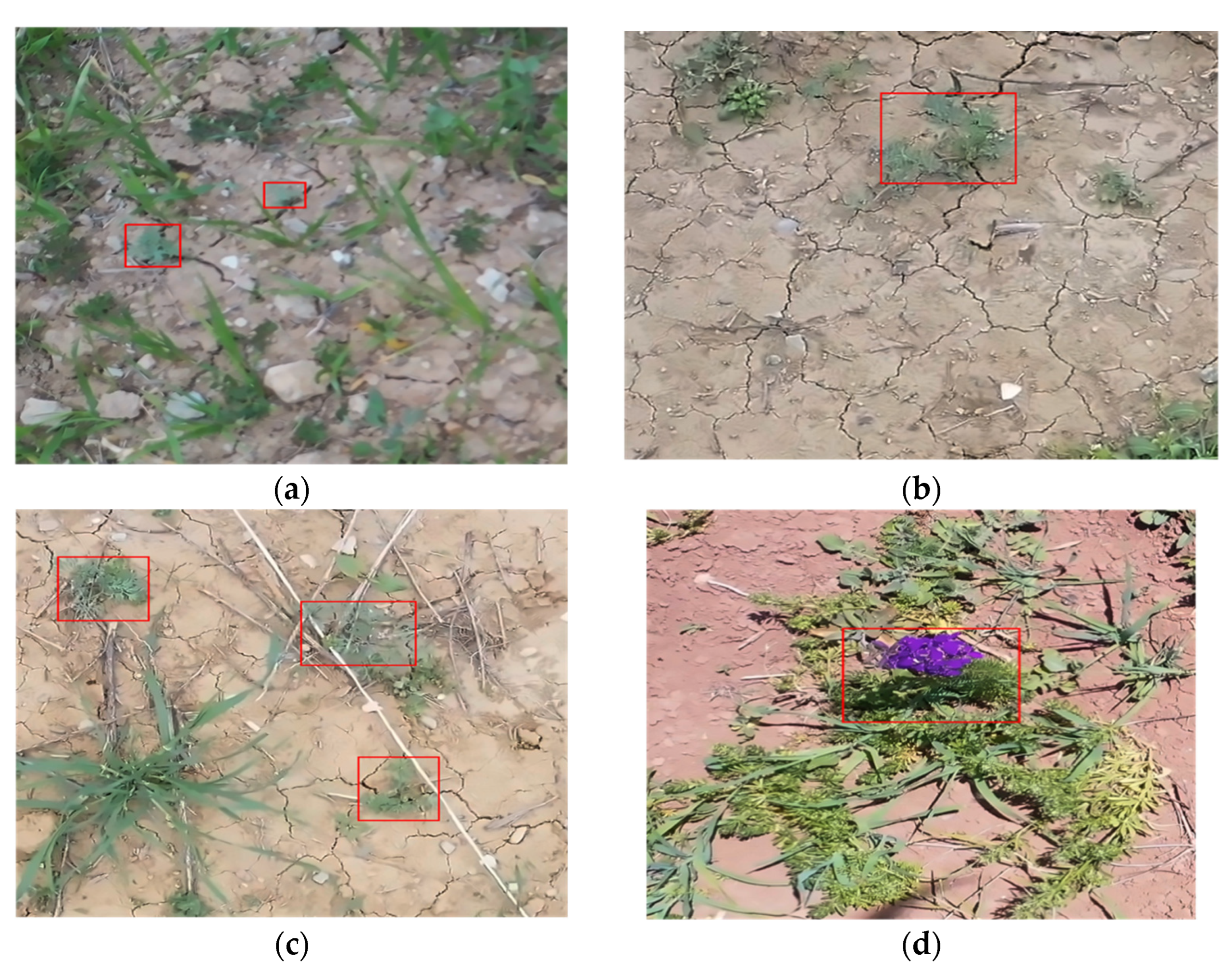
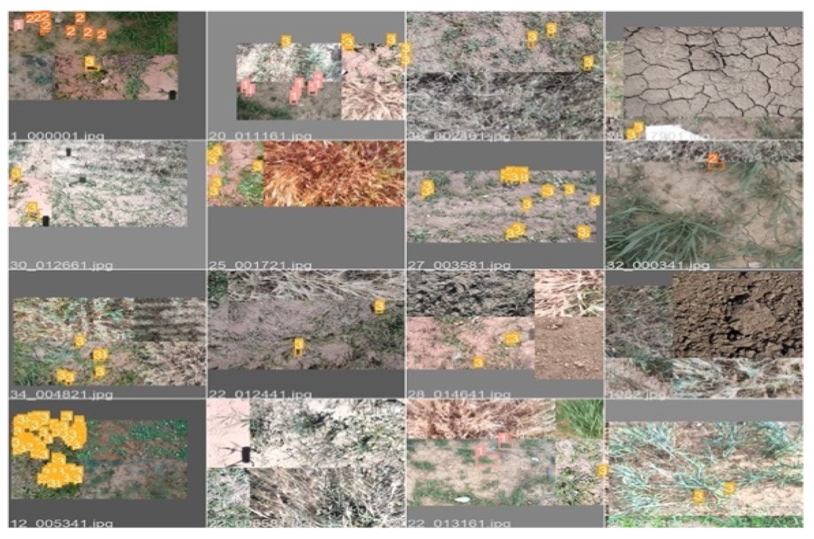
2.1. Dataset
2.2. Weed Object Detectors
2.2.1. One-Stage Weed Detectors
YOLOv5
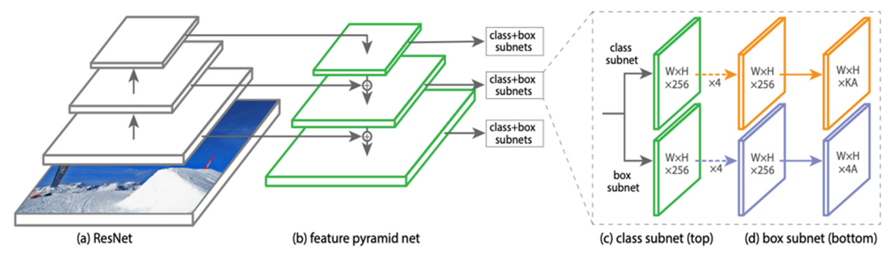
RetinaNet
2.2.2. Two-Stage Weed Detectors
Faster R-CNN
3. Training and Testing
3.1. Setup
3.2. Performance Evaluation Metrics
4. Results
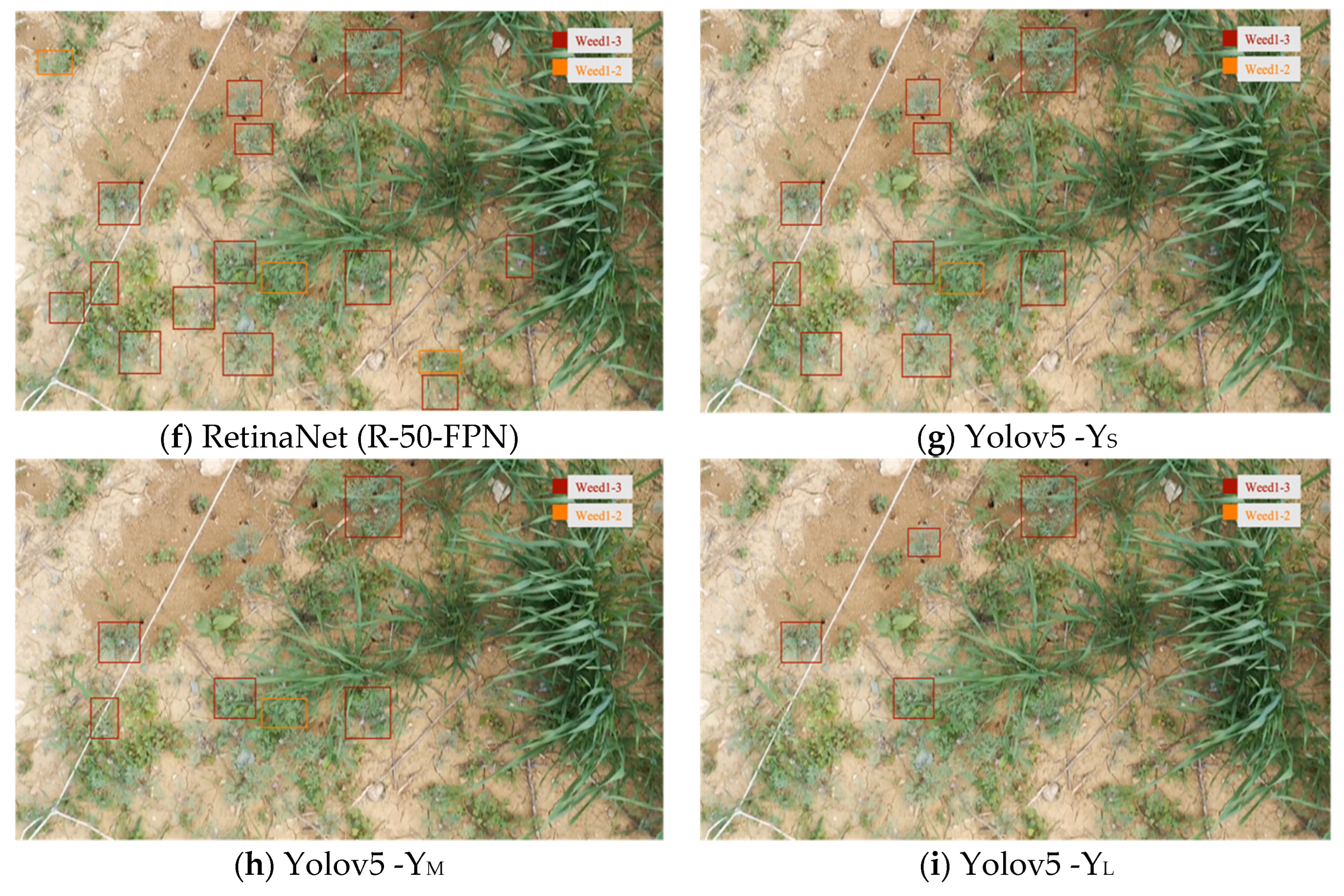
4.1. YOLOv5 Weed Detection and Classification Results
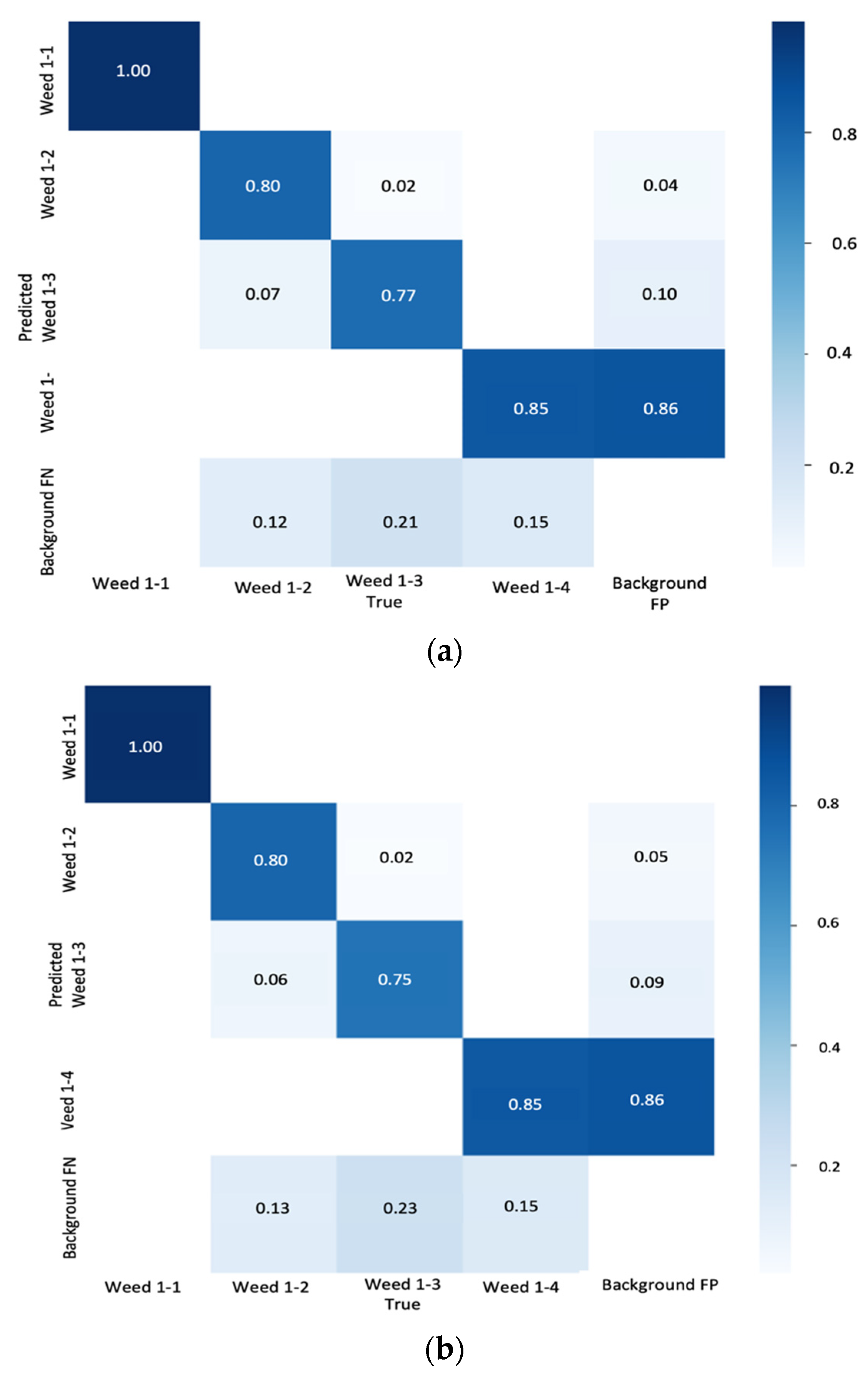
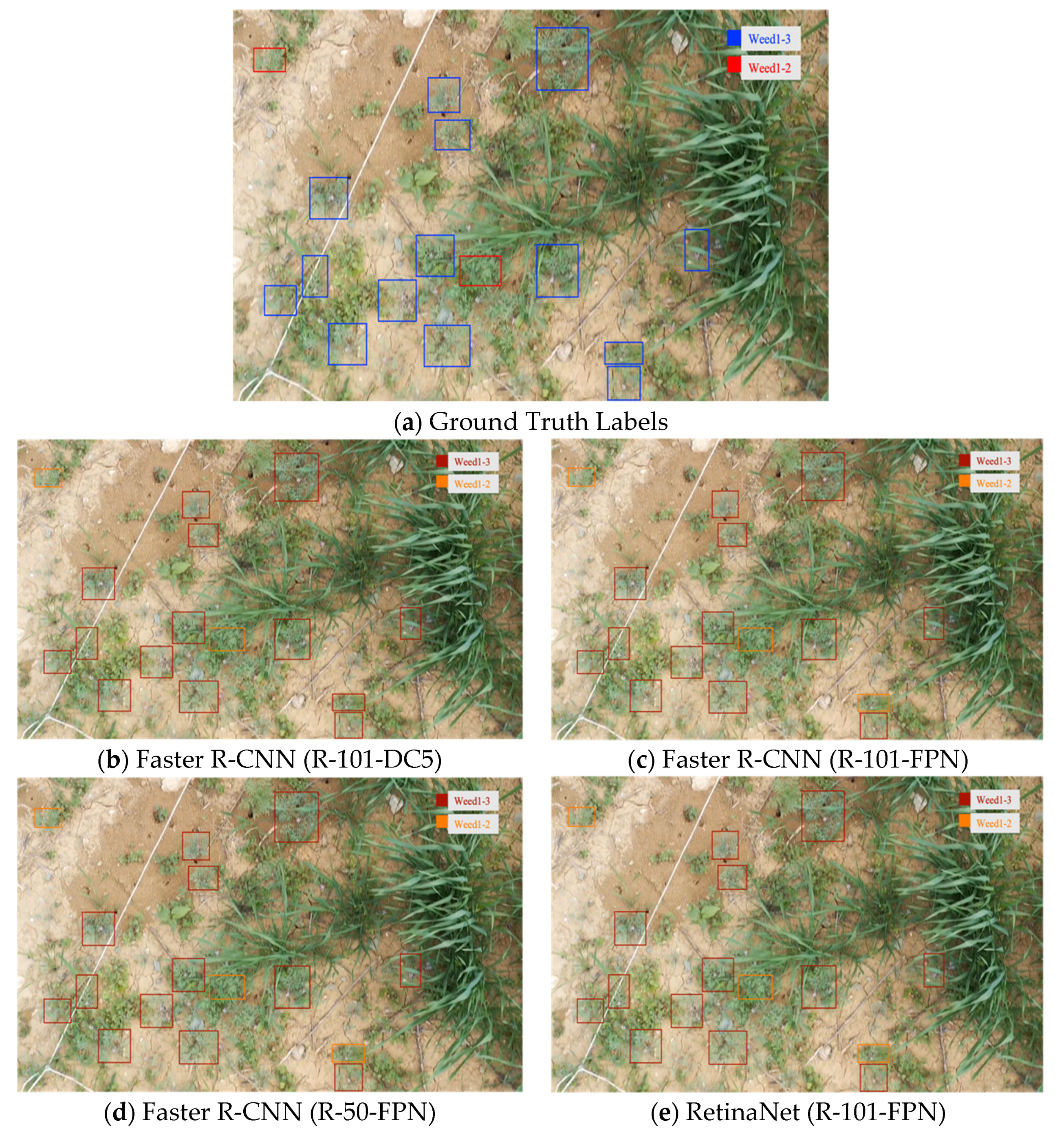
4.2. Faster R-CNN and RetinaNet Weed Detection and Classification Results
4.3. Weed Detection and Growth Stages Classification Results
5. Discussion
6. Conclusions
Author Contributions
Funding
Data Availability Statement
Acknowledgments
Conflicts of Interest
References
- Sylvester, G. E-Agriculture in Action: Drones for Agriculture; Food and Agriculture Organization of the United Nations: Bangkok, Thailand, 2018. [Google Scholar]
- Lee, W.S.; Alchanatis, V.; Yang, C.; Hirafuji, M.; Moshou, D.; Li, C. Sensing Technologies for Precision Specialty Crop Production. Comp. Elect. Agric. 2010, 74, 2–33. [Google Scholar] [CrossRef]
- Swanton, C.J.; Nkoa, R.; Blackshaw, R.E. Experimental Methods for Crop–Weed Competition Studies. Weed Sci. 2015, 63, 2–11. [Google Scholar] [CrossRef] [Green Version]
- Patel, D.D.; Kumbhar, B.A. Weed and Its Management: A Major Threats to Crop Economy. J. Pharm. Sci. Biosci. Res. 2016, 6, 753–758. [Google Scholar]
- Pimentel, D.; Zuniga, R.; Morrison, D. Update on the Environmental and Economic Costs Associated with Alien-Invasive Species in the United States. Ecol. Econ. 2005, 52, 273–288. [Google Scholar] [CrossRef]
- Ghardea, Y.; Singha, P.K.; Dubeya, R.P.; Gupta, P.K. Assessment of yield and economic losses in agriculture due to weeds in India. Sci. Direct 2018, 107, 12–18. [Google Scholar] [CrossRef]
- Methods of Weed Control. Available online: https://www.larimer.gov/naturalresources/weeds/control (accessed on 25 September 2022).
- Holt, J.S. Principles of Weed Management in Agroecosystems and Wildlands. Weed Technol. 2004, 18, 1559–1562. [Google Scholar] [CrossRef]
- Llewellyn, R.; Ronning, D.; Clarke, M.; Mayfield, A.; Walker, S.; Ouzman, J. Impact of Weeds on Australian Grain Production—The Cost of Weeds to Australian Grain Growers and the Adoption of Weed Management and Tillage Practices; Grains Research and Development Corporation and the Commonwealth Scientific and Industrial Research Organisation: Canberra, Australia, 2016. [Google Scholar]
- Bàrberi, P. Weed Management in Organic Agriculture: Are We Addressing the Right Issues? Weed Res. 2002, 42, 177–193. [Google Scholar] [CrossRef]
- Lameski, P.; Zdravevski, E.; Kulakov, A. A Short Review of the Environmental Impact of Automated Weed Control. In ICT Innovations 2018; Engineering and Life Sciences; Springer: Cham, Switzerland, 2018; pp. 132–147. [Google Scholar]
- Paikekari, A.; Ghule, V.; Meshram, R.; Raskar, V. Weed Detection Using Image Processing. Inter. Res. J. Eng. Technol. 2016, 3, 1220–1222. [Google Scholar]
- Tang, J.-L.; Chen, X.-Q.; Miao, R.-H.; Wang, D. Weed Detection Using Image Processing under Different Illumination for Site-Specific Areas Spraying. Comput. Elect. Agric. 2016, 122, 103–111. [Google Scholar] [CrossRef]
- Burgos-Artizzu, X.P.; Ribeiro, A.; Guijarro, M.; Pajares, G. Real-Time Image Processing for Crop/Weed Discrimination in Maize Fields. Comput. Elect. Agric. 2011, 75, 337–346. [Google Scholar] [CrossRef] [Green Version]
- Hameed, S.; Amin, I. Detection of Weed and Wheat Using Image Processing. In Proceedings of the 2018 IEEE 5th International Conference on Engineering Technologies and Applied Sciences (ICETAS), Bangkok, Thailand, 22–23 November 2018; pp. 1–5. [Google Scholar] [CrossRef]
- Pérez, A.J.; López, F.; Benlloch, J.V.; Christensen, S. Colour and Shape Analysis Techniques for Weed Detection in Cereal Fields. Comput. Elect. Agric. 2000, 25, 197–212. [Google Scholar] [CrossRef]
- Tejeda, A.J.I.; Castro, R.C. Algorithm of Weed Detection in Crops by Computational Vision. In Proceedings of the 2019 International Conference on Electronics, Communications and Computers (CONIELECOMP), IEEE, Cholula, Mexico, 27 February–1 March 2019; pp. 124–128. [Google Scholar] [CrossRef]
- Parra, L.; Torices, V.; Marín, J.; Mauri, P.V.; Lloret, J. The Use of Image Processing Techniques for Detection of Weed in Lawns. In Proceedings of the Fourteenth International Conference on Systems (ICONS 2019), Valencia, Spain, 24–28 March 2019; pp. 24–28. [Google Scholar]
- Bini, D.; Pamela, D.; Prince, S. Machine vision and machine learning for intelligent agrobots: A review. In Proceedings of the 2020 5th International Conference on Devices, Circuits and Systems (ICDCS), Coimbatore, India, 5–6 March 2020; pp. 12–16. [Google Scholar]
- César Pereira Júnior, P.; Monteiro, A.; Da Luz Ribeiro, R.; Sobieranski, A.C.; Von Wangenheim, A. Comparison of Supervised Classifiers and Image Features for Crop Rows Segmentation on Aerial Images. Appl. Artif. Intell. 2020, 34, 271–291. [Google Scholar] [CrossRef]
- Pantazi, X.E.; Tamouridou, A.A.; Alexandridis, T.K.; Lagopodi, A.L.; Kashefi, J.; Moshou, D. Evaluation of Hierarchical Self-Organising Maps for Weed Mapping Using UAS Multispectral Imagery. Comput. Elect. Agric. 2017, 139, 224–230. [Google Scholar] [CrossRef]
- Pantazi, X.-E.; Moshou, D.; Bravo, C. Active Learning System for Weed Species Recognition Based on Hyperspectral Sensing. Biosyst. Engin. 2016, 146, 193–202. [Google Scholar] [CrossRef]
- Binch, A.; Fox, C.W. Controlled Comparison of Machine Vision Algorithms for Rumex and Urtica Detection in Grassland. Comput. Elect. Agric. 2017, 140, 123–138. [Google Scholar] [CrossRef] [Green Version]
- Alam, M.; Alam, M.S.; Roman, M.; Tufail, M.; Khan, M.U.; Khan, M.T. Real-Time Machine-Learning Based Crop/Weed Detection and Classification for Variable-Rate Spraying in Precision Agriculture. In Proceedings of the 2020 7th International Conference on Electrical and Electronics Engineering (ICEEE), IEEE, Antalya, Turkey, 14–16 April 2020; pp. 273–280. [Google Scholar] [CrossRef]
- Islam, N.; Rashid, M.M.; Wibowo, S.; Xu, C.-Y.; Morshed, A.; Wasimi, S.A.; Moore, S.; Rahman, S.M. Early Weed Detection Using Image Processing and Machine Learning Techniques in an Australian Chilli Farm. Agriculture 2021, 11, 387. [Google Scholar] [CrossRef]
- Gao, J.; Nuyttens, D.; Lootens, P.; He, Y.; Pieters, J.G. Recognizing Weeds in a Maize Crop Using a Random Forest Machine-Learning Algorithm and near-Infrared Snapshot Mosaic Hyperspectral Imagery. Biosyst. Eng. 2018, 170, 39–50. [Google Scholar] [CrossRef]
- Liu, L.; Ouyang, W.; Wang, X.; Fieguth, P.; Chen, J.; Liu, X.; Pietikäinen, M. Deep Learning for Generic Object Detection: A Survey. Int. J. Comput. Vis. 2020, 128, 261–318. [Google Scholar] [CrossRef] [Green Version]
- Redmon, J.; Divvala, S.; Girshick, R.; Farhadi, A. You Only Look Once: Unified, Real-Time Object Detection. In Proceedings of the 2016 IEEE Conference on Computer Vision and Pattern Recognition (CVPR), IEEE, Los Alamitos, CA, USA, 27–30 June 2016; pp. 779–788. [Google Scholar] [CrossRef] [Green Version]
- Liu, W.; Anguelov, D.; Erhan, D.; Szegedy, C.; Reed, S.; Fu, C.-Y.; Berg, A.C. SSD: Single Shot MultiBox Detector. In Proceedings of the Computer Vision—ECCV 2016, Amsterdam, The Netherlands, 11–14 October 2016; Leibe, B., Matas, J., Sebe, N., Welling, M., Eds.; Springer International Publishing: Cham, Switzerland, 2016; pp. 21–37. [Google Scholar] [CrossRef] [Green Version]
- Ren, S.; He, K.; Girshick, R.; Sun, J. Faster R-CNN: Towards Real-Time Object Detection with Region Proposal Networks. IEEE Trans. Neural Netw. 2017, 39, 1137–1149. [Google Scholar] [CrossRef] [Green Version]
- Yu, J.; Sharpe, S.M.; Schumann, A.W.; Boyd, N.S. Deep Learning for Image-Based Weed Detection in Turfgrass. Eur. J. Agron. 2019, 104, 78–84. [Google Scholar] [CrossRef]
- Veeranampalayam Sivakumar, A.N.; Li, J.; Scott, S.; Psota, E.; Jhala, J.A.; Luck, J.D.; Shi, Y. Comparison of Object Detection and Patch-Based Classification Deep Learning Models on Mid- to Late-Season Weed Detection in UAV Imagery. Remote Sens. 2020, 12, 2136. [Google Scholar] [CrossRef]
- Dyrmann, M.; Jørgensen, R.N.; Midtiby, H.S. RoboWeedSupport—Detection of Weed Locations in Leaf Occluded Cereal Crops Using a Fully Convolutional Neural Network. Adv. Anim. Biosci. 2017, 8, 842–847. [Google Scholar] [CrossRef]
- Sharpe, S.M.; Schumann, A.W.; Yu, J.; Boyd, N.S. Vegetation Detection and Discrimination within Vegetable Plasticulture Row-Middles Using a Convolutional Neural Network. Precis. Agric. 2020, 21, 264–277. [Google Scholar] [CrossRef]
- Junior, L.C.M.; Ulson, J.A.C. Real Time Weed Detection Using Computer Vision and Deep Learning. In Proceedings of the 2021 14th IEEE International Conference on Industry Applications (INDUSCON), IEEE, São Paulo, Brazil, 16–18 August 2021; pp. 1131–1137. [Google Scholar] [CrossRef]
- Salazar-Gomez, A.; Darbyshire, M.; Gao, J.; Sklar, E.I.; Parsons, S. Towards Practical Object Detection for Weed Spraying in Precision Agriculture. arXiv 2021. [Google Scholar] [CrossRef]
- Subeesh, A.; Bhole, S.; Singh, K.; Chandel, N.S.; Rajwade, Y.A.; Rao, K.V.R.; Kumar, S.P.; Jat, D. Deep Convolutional Neural Network Models for Weed Detection in Polyhouse Grown Bell Peppers. Artif. Intell. Agric. 2022, 6, 47–54. [Google Scholar] [CrossRef]
- Saleem, M.H.; Potgieter, J.; Arif, K.M. Weed Detection by Faster RCNN Model: An Enhanced Anchor Box Approach. Agronomy 2022, 12, 1580. [Google Scholar] [CrossRef]
- Quan, L.; Feng, H.; Lv, Y.; Wang, Q.; Zhang, C.; Liu, J.; Yuan, Z. Maize Seedling Detection under Different Growth Stages and Complex Field Environments Based on an Improved Faster R-CNN. Biosyst. Eng. 2019, 184, 1–23. [Google Scholar] [CrossRef]
- Teimouri, N.; Jørgensen, R.N.; Green, O. Novel Assessment of Region-Based CNNs for Detecting Monocot/Dicot Weeds in Dense Field Environments. Agronomy 2022, 12, 1167. [Google Scholar] [CrossRef]
- Chen, D.; Lu, Y.; Li, Z.; Young, S. Performance Evaluation of Deep Transfer Learning on Multi-Class Identification of Common Weed Species in Cotton Production Systems. Comput. Elect. Agric. 2022, 198, 107091. [Google Scholar] [CrossRef]
- Mahmudul Hasan, A.S.M.; Sohel, F.; Diepeveen, D.; Laga, H.; Jones, M.G.K. Weed Recognition Using Deep Learning Techniques on Class-Imbalanced Imagery. Crop Pasture Sci. 2022, A–Q. [Google Scholar] [CrossRef]
- Jin, X.; Bagavathiannan, M.; Maity, A.; Chen, Y.; Yu, J. Deep Learning for Detecting Herbicide Weed Control Spectrum in Turfgrass. Plant Methods 2022, 18, 94. [Google Scholar] [CrossRef] [PubMed]
- Teimouri, N.; Dyrmann, M.; Nielsen, P.R.; Mathiassen, S.K.; Somerville, G.J.; Jørgensen, R.N. Weed Growth Stage Estimator Using Deep Convolutional Neural Networks. Sensors 2018, 18, 1580. [Google Scholar] [CrossRef] [Green Version]
- Mishra, A.M.; Harnal, S.; Mohiuddin, K.; Gautam, V.; Nasr, O.A.; Goyal, N.; Alwetaishi, M.; Singh, A. A Deep Learning-Based Novel Approach for Weed Growth Estimation. Intell. Autom. Soft Comput. 2022, 31, 1157–1173. [Google Scholar] [CrossRef]
- Hasan, A.S.M.M.; Sohel, F.; Diepeveen, D.; Laga, H.; Jones, M.G.K. A Survey of Deep Learning Techniques for Weed Detection from Images. Comput. Elect. Agric. 2021, 184, 106067. [Google Scholar] [CrossRef]
- Almalky, A.M.; Ahmed, K.R.; Guzel, M.; Turan, B. An Efficient Deep Learning Technique for Detecting and Classifying the Growth of Weeds on Fields. In Proceedings of the Future Technologies Conference (FTC) 2022, Volume 2; Arai, K., Ed.; Lecture Notes in Networks and Systems; Springer International Publishing: Cham, Switzerland, 2023; pp. 818–835. [Google Scholar] [CrossRef]
- Jocher, G. Yolov5. Available online: https://github.com/ultralytics/yolov5 (accessed on 25 March 2022).
- Lin, T.; Goyal, P.; Girshick, R.; He, K.; Dollar, P. Focal Loss for Dense Object Detection. IEEE Trans. Pattern Anal. Mach. Intell. 2020, 42, 318–327. [Google Scholar] [CrossRef] [Green Version]
- Lin, T. LabelImg. Available online: https://github.com/tzutalin/labelImg (accessed on 20 April 2022).
- Chen, X.-W.; Lin, X. Big Data Deep Learning: Challenges and Perspectives. IEEE Access 2014, 2, 514–525. [Google Scholar] [CrossRef]
- Redmon, J.; Farhadi, A. YOLO9000: Better, Faster, Stronger. In Proceedings of the 2017 IEEE Conference on Computer Vision and Pattern Recognition (CVPR), IEEE, Honolulu, HI, USA, 21–26 July 2017; pp. 6517–6525. [Google Scholar] [CrossRef] [Green Version]
- Redmon, J.; Farhadi, A. YOLOv3: An Incremental Improvement. arXiv 2018. [Google Scholar] [CrossRef]
- Bochkovskiy, A.; Wang, C.-Y.; Liao, H.-Y.M. YOLOv4: Optimal Speed and Accuracy of Object Detection. arXiv 2020. [Google Scholar] [CrossRef]
- Zhu, L.; Geng, X.; Li, Z.; Liu, C. Improving YOLOv5 with Attention Mechanism for Detecting Boulders from Planetary Images. Remote Sens. 2021, 13, 3776. [Google Scholar] [CrossRef]
- Wang, C.-Y.; Mark Liao, H.-Y.; Wu, Y.-H.; Chen, P.-Y.; Hsieh, J.-W.; Yeh, I.-H. CSPNet: A New Backbone That Can Enhance Learning Capability of CNN. In Proceedings of the 2020 IEEE/CVF Conference on Computer Vision and Pattern Recognition Workshops (CVPRW), IEEE, Seattle, WA, USA, 14–19 June 2020; pp. 1571–1580. [Google Scholar] [CrossRef]
- Lin, T.-Y.; Dollar, P.; Girshick, R.; He, K.; Hariharan, B.; Belongie, S. Feature Pyramid Networks for Object Detection. In Proceedings of the 2017 IEEE Conference on Computer Vision and Pattern Recognition (CVPR), IEEE, Honolulu, HI, USA, 21–26 July 2017; pp. 936–944. [Google Scholar] [CrossRef] [Green Version]
- He, K.; Zhang, X.; Ren, S.; Sun, J. Deep Residual Learning for Image Recognition. In Proceedings of the 2016 IEEE Conference on Computer Vision and Pattern Recognition (CVPR), IEEE, Las Vegas, NV, USA, 27–30 June 2016; pp. 770–778. [Google Scholar] [CrossRef] [Green Version]
- Girshick, R. Fast R-CNN. In Proceedings of the 2015 IEEE International Conference on Computer Vision (ICCV), IEEE, Santiago, Chile, 11–18 December 2015; pp. 1440–1448. [Google Scholar] [CrossRef]
- Liu, S.; Deng, W. Very Deep Convolutional Neural Network Based Image Classification Using Small Training Sample Size. In Proceedings of the 2015 3rd IAPR Asian Conference on Pattern Recognition (ACPR), IEEE, Kuala Lumpur, Malaysia, 3–6 November 2015; pp. 730–734. [Google Scholar] [CrossRef]
- Howard, A.G.; Zhu, M.; Chen, B.; Kalenichenko, D.; Wang, W.; Weyand, T.; Andreetto, M.; Adam, H. MobileNets: Efficient Convolutional Neural Networks for Mobile Vision Applications. arXiv 2017. [Google Scholar] [CrossRef]
- Bradski, G. The OpenCV Library. Dr. Dobb’s J. Softw. Tools Prof. Program 2000, 25, 120–123. [Google Scholar]
- Ketkar, N. Deep Learning with Python: A Hands-on Introduction, 3rd ed.; Apress: New York, NY, USA, 2017; pp. 195–208. ISBN 978-1-4842-2765-7. [Google Scholar]
- Kirk, D. NVIDIA Cuda Software and Gpu Parallel Computing Architecture. In Proceedings of the 6th International Symposium on Memory Management, Montreal, QC, Canada, 21–22 October 2007; Association for Computing Machinery: New York, NY, USA, 2007; pp. 103–104. [Google Scholar] [CrossRef]
- Oliphant, T.E. Guide to NumPy, 2nd ed.; CreateSpace Independent Publishing Platform: Scotts Valley, CA, USA, 2015. [Google Scholar]
- Abadi, M.; Agarwal, A.; Barham, P.; Brevdo, E.; Chen, Z.; Citro, C.; Corrado, G.S.; Davis, A.; Dean, J.; Devin, M.; et al. TensorFlow: Large-Scale Machine Learning on Heterogeneous Distributed Systems. arXiv 2016. [Google Scholar] [CrossRef]
- Wu, Y.; Kirillov, A.; Massa, F.; Lo, W.-Y.; Girshick, R. Detectron2. 2019. Available online: https://github.com/facebookresearch/detectron2 (accessed on 14 September 2022).


| Ref. | Pre-Processing | Programming Language/Method |
|---|---|---|
| [12] | Color segmentation, edge detection and filtering. | MATLAB |
| [13] | Selecting YCrCb color space and Cg component, calculating the line in the middle of crop, calculating minimum error ratio of Bayesian decision. | Bayesian decision |
| [14] | Color segmentation, dividing images into horizontal strips, creating component vector for each strip. | C++ |
| [15] | Edge detection, background subtraction. | MATLAB |
| [16] | Analyzing differences in spectral reflectance between vegetation and soil, image segmentation using morphological dilation. | Bayes Rule and the k-Nearest Neighbor (KNN) |
| [17] | Subtracting the green parts in the image, filtering using medium and morphological filters. | MATLAB |
| [18] | Background removal, RGB images acquisition. | Two suggested equations |
| Ref. | Extracted Features/Segmentation Method | Models | Best Result |
|---|---|---|---|
| [19] | Local binary pattern (LBP) segmentation. | Support Vector Machine (SVM) | Not mentioned |
| [20] | Vegetation indices for color features extraction, gray level co-occurrence matrices (GLCM), Gabor filters. | SVM, Random Forest (RF) Mahalanobis Classifier (MC), KNN | F1_score = 88% by SVM model |
| [21] | Three spectral bands of Red, Green, Near Infrared (NIR), texture layer. | Supervised Kohonen Network (SKN), Counter-propagation Artificial Neural Network (CP-ANN), XY-Fusion network (XY-F) | Accuracy = 98.87% by CP-ANN model |
| [22] | Spectral reflectance. | Mixture of Gaussians (MOG), one-class self-organizing map (SOM) classifiers, one-class SVM | Performance = 31–98% by MOG model |
| [23] | Linear binary patterns, BRISK, Fourier analysis, watershed. | SVM, linear discriminants KNN, meta-classifier combinations | SVM model showed best result |
| [24] | Color-based segmentation, watershed segmentation, edge-based segmentation, Hu moments for analyzing leaf shape. | RF | Accuracy = 95% by RF. |
| [25] | Converting images to orthomosaic images, extracting RGB-band reflectance. | RF, SVM, KNN | Accuracy = 96% by RF. |
| [26] | 185 spectral features (including reflectance and vegetation index features). | RF | Precision = 94% in detecting crops, and 95.9% in detecting weeds. |
| Ref. | Models | Best Result |
|---|---|---|
| [31] | Google-Net, Visual Geometry Group Net (VGG-Net), Detect-Net | F1_score > 0.99 by Detect-Net |
| [32] | Faster R-CNN, SSD | Faster R-CNN model showed best result |
| [33] | Google-Net | Accuracy = 86.6% |
| [34] | YOLOV3 | F1_score = 0.95 |
| [35] | YOLOV5 | Accuracy = 77% |
| [36] | YOLOV5-medium, YOLOV3, YOLOV4, Faster R-CNN | Mean Average Precision (mAp) = 87.5 by YOLOV5-medium |
| [37] | Alex-net, Google-Net, Inception-V3, Xception | Accuracy = 97.7% by Inception-V3 |
| [38] | Faster R-CNN with different anchor box scales and aspect ratios | mAP = 96.02 with the addition of 64 × 64 scale size, and aspect ratio of 1:3 and 3:1 |
| [39] | Faster R-CNN with different backbones (Alexnet, VGG16, VGG19, Squeezeenet, Googlenet, Inceptionv3, Mobilenetv2, Resnet18, Resnet50, and Resnet101) | Precision = 0.98, recall = 0.96 by Faster R-CNN with VGG19 |
| [40] | EfficientDet (coefficient 3), YOLOv5 | AP for detecting monocot/dicot = 30.70 /51.50% by YOLOv5 |
| [41] | Tested 27 DL models | F1 = 99.1% by ResNet101 |
| [42] | VGG16, ResNet-50, Inception-V3, Inception-ResNet-v2 MobileNetV2 | Average precision = 98.29, recall = 98.30 by Resnet-50 |
| [43] | GoogLeNet, MobileNet-v3, ShuffleNet-v2, VGG-Net | Accuracy ≥ 0.999, F1 ≥ 0.998 by ShuffleNet-v2 and VGG-Net |
| [44] | Inception-v3 | Accuracy = 70% |
| [45] | Inception-V4, Efficient-NetB7 | Accuracy = 70% by Efficient-NetB7 |
| Sensor | 1″ CMOS, Effective Pixels: 20 million |
| Lens | FOV: about 77°, 35 mm Format Equivalent: 28 mm Aperture: f/2.8–f/11, Shooting Range: 1 m to ∞ |
| ISO Range | Video: 100–6400, Photo: 100–3200 (auto), 100–12,800 (manual) |
| Still Image Size | 5472 × 3648 |
| Video Resolution | 4K: 3840 × 2160 24/25/30p, 2.7K: 2688 × 1512 24/25/30/48/50/60p FHD: 1920 × 1080 24/25/30/48/50/60/120p |
| Place | Turkey |
| Time for Collecting Dataset | One year and six months |
| Number of Recorded Videos | 47 videos |
| Videos Duration | ~5 min/each video |
| Number of Instances |
|
| YOLOv5 | Precision | Recall | mAP@.5 | mAP@.5:.95 | F1 | Size in Megabytes | Inference Time (s) | Training Time (h) |
|---|---|---|---|---|---|---|---|---|
| Ys | 0.788 | 0.794 | 0.805 | 0.363 | 0.79 | 14.342 MB | 0.0064 | 9.598 |
| YM | 0.809 | 0.775 | 0.808 | 0.351 | 0.79 | 41.493 MB | 0.0097 | 10.161 |
| YL | 0.827 | 0.779 | 0.816 | 0.382 | 0.80 | 90.957 MB | 0.0142 | 9.365 |
| Classes | Precision | Recall | mAP@.5 | mAP@.5:.95 | ||||||||
|---|---|---|---|---|---|---|---|---|---|---|---|---|
| Ys | YM | YL | Ys | YM | YL | Ys | YM | YL | Ys | YM | YL | |
| Weed 1-1 | 0.907 | 0.914 | 0.966 | 1 | 1 | 1 | 0.976 | 0.995 | 0.995 | 0.495 | 0.443 | 0.552 |
| Weed 1-2 | 0.773 | 0.783 | 0.807 | 0.744 | 0.718 | 0.702 | 0.777 | 0.783 | 0.785 | 0.373 | 0.38 | 0.386 |
| Weed 1-3 | 0.716 | 0.751 | 0.733 | 0.682 | 0.659 | 0.683 | 0.716 | 0.696 | 0.715 | 0.305 | 0.303 | 0.307 |
| Weed 1-4 | 0.756 | 0.789 | 0.802 | 0.749 | 0.723 | 0.732 | 0.752 | 0.757 | 0.77 | 0.278 | 0.277 | 0.282 |
| Model | Backbone | AP@50 | AP@.5:.95 | Recall | Size in Megabytes | F1 | Inference Time (s) | Training Time (h) |
|---|---|---|---|---|---|---|---|---|
| Faster R-CNN | R-101-DC5 1 | 86.32 | 37.464 | 60.037 | 1438.699 | 0.70 | 0.0924 | 11:52:57 |
| Faster R-CNN | R-101-FPN 2 | 86.763 | 47.170 | 62.1 | 815.742 | 0.72 | 0.08727 | 16:18:44 |
| Faster R-CNN | R-50-FPN 3 | 84.165 | 38.039 | 54.5 | 322.410 | 0.66 | 0.0917 | 9:11:18 |
| RetinaNet | R-101-FPN 2 | 87.457 | 49.991 | 65.5 | 432.056 | 0.74 | 0.09130 | 9:19:56 |
| RetinaNet | R-50-FPN 3 | 86.404 | 45.156 | 62.4 | 283.574 | 0.72 | 0.0889 | 8:38:46 |
| Model | Backbone | Weed 1-1 | Weed 1-2 | Weed 1-3 | Weed 1-4 |
|---|---|---|---|---|---|
| Faster R-CNN | R-101-DC5 | 42.624 | 58.022 | 47.045 | 30.216 |
| Faster R-CNN | R-101-FPN | 50.099 | 58.817 | 48.419 | 31.346 |
| Faster R-CNN | R-50-FPN | 35.050 | 52.184 | 38.732 | 26.192 |
| RetinaNet | R-101-FPN | 55.149 | 57.098 | 55.809 | 31.910 |
| RetinaNet | R-50-FPN | 45.149 | 55.730 | 50.702 | 29.043 |
Disclaimer/Publisher’s Note: The statements, opinions and data contained in all publications are solely those of the individual author(s) and contributor(s) and not of MDPI and/or the editor(s). MDPI and/or the editor(s) disclaim responsibility for any injury to people or property resulting from any ideas, methods, instructions or products referred to in the content. |
© 2023 by the authors. Licensee MDPI, Basel, Switzerland. This article is an open access article distributed under the terms and conditions of the Creative Commons Attribution (CC BY) license (https://creativecommons.org/licenses/by/4.0/).
Share and Cite
Almalky, A.M.; Ahmed, K.R. Deep Learning for Detecting and Classifying the Growth Stages of Consolida regalis Weeds on Fields. Agronomy 2023, 13, 934. https://doi.org/10.3390/agronomy13030934
Almalky AM, Ahmed KR. Deep Learning for Detecting and Classifying the Growth Stages of Consolida regalis Weeds on Fields. Agronomy. 2023; 13(3):934. https://doi.org/10.3390/agronomy13030934
Chicago/Turabian StyleAlmalky, Abeer M., and Khaled R. Ahmed. 2023. "Deep Learning for Detecting and Classifying the Growth Stages of Consolida regalis Weeds on Fields" Agronomy 13, no. 3: 934. https://doi.org/10.3390/agronomy13030934