Study on the In-Field Water Balance of Direct-Seeded Rice with Various Irrigation Regimes under Arid Climatic Conditions in Egypt Using the AquaCrop Model

Abstract

Crop growth models are cost-effective and user-friendly tools for decision-makers to develop efficient in-field management strategies. These models are particularly important in countries such as Egypt, where the risk of water scarcity is inevitable. The present study aimed to examine the in-field water balance of direct-seeded rice (Giza 178) under various irrigation regimes and arid conditions during two growing seasons (2019 and 2020). Four irrigation regimes, namely, continuous flood irrigation with a fixed water depth of 5 cm, and 3-, 6-, and 10-day irrigation frequencies (FI, 3IF, 6IF, and 10IF, respectively), were arranged in a randomized complete block design with three replicates. Then, the feasibility of using AquaCrop in simulating direct-seeded rice development and in-field water balance was assessed. Five statistical indicators, including normalized root-mean-squared error (NRMSE), index of agreement (d), coefficient of determination (R²), Nash–Sutcliffe efficiency coefficient (EF), and percent deviation (P_d), were used to evaluate the performance of AquaCrop. The field trial results demonstrated that both the 3IF and 6IF irrigation regimes were the best for achieving the highest biomass (21.0 t·ha⁻¹, under 3IF), yield (9.8 t·ha⁻¹, under 3IF), and saving irrigation water (18.3–22.4%, under 6IF), making them the best to apply in Egypt. Moreover, the AquaCrop simulation results showed a good correlation between the observed and simulated rice yield (Y) in both seasons (R² = 0.99 and 0.98 in 2019 and 2020, respectively). AquaCrop showed excellent performance in simulating canopy cover (CC) and biomass (B) during both growing seasons (5.0 ≤ NRMSE ≤ 15.0, 0.97 ≤ d ≤ 0.99, 0.92 ≤ R² ≤ 0.99, and 0.92 ≤ EF ≤ 0.99). In addition, the model showed acceptable performance in simulating in-field water balance components. Reasonably good model efficiency was recorded in simulating crop actual evapotranspiration (ET_act). Meanwhile, the average P_d for percolation (P) was between −15.3% and 5.4% during both growing seasons. Overall, AquaCrop showed adequate accuracy in simulating CC, B, Y, ET_act, and P but relatively low efficiency in simulating ET_act and P under severe water scarcity. Therefore, AquaCrop may serve as a valuable tool for irrigation management and crop yield prediction even in arid regions, such as Egypt.

1. Introduction

While the agriculture sector faces many challenges, the most critical one is ensuring food security with the rapid increase in population and water scarcity around the world. Paddy rice (Oryza sativa L.) is an important field crop, covering around 160 Mha of agricultural land and is an essential food source for approximately 3.5 billion people worldwide [1,2,3,4]. Rice cultivation consumes most of the fresh water dedicated to irrigation worldwide. Egypt is classified as one of the 35 water-deficit countries [5]. In Egypt, agricultural land accounts for only approximately 4% of the total area of the country, while the remaining part is an arid desert [6]. Rice is typically cultivated in the Nile River Delta (NRD) region under flooded conditions, with nearly 5 cm of stagnant water during the cultivation season from May to October [2] and consuming about 20% of Egypt’s water resource supply from the Nile River (11 billion m³.year⁻¹) [7].

Recently, new high-yielding, short-lived genotypes, such as Giza 177, 178, and 182, Sakha 101, 102, 103, and 104, and Egyptian Yasmine were released and spread to guarantee food security and tackle water scarcity problems. As a result, the total national rice productivity reached 7.1 million tons, with an average of 9.9 t·ha⁻¹ in 2012, rendering the country’s average rice productivity the highest in the world [8]. However, Egypt produces only about 60% of its food and 40% of its grain needs [9]. According to statistical reports, by 2050, agricultural production must increase by 70% to achieve food security [10]. Therefore, stress on rice production is high owing to the potential risk of worsening water deficit due to climate change and limited cropland. Furthermore, the agricultural sector, which consumes 87.7% of the total water resources, is primarily affected by the construction of the Ethiopian Renaissance Dam (ERD) on the Nile River. Egypt depends on the Nile River for 97% of its water requirements, while approximately 86% of the Nile water flows from the Ethiopian Plateau. With damming, approximately 1.7 Mha of the cultivated area is expected to undergo desertification due to water shortage, accompanied by a potential decrease in all crop yields and an increase in irrigation requirements due to climate change [5]. Consequently, a better balance between the available irrigation resources and plant water requirements with a deeper understanding of water use efficiency (WUE) and water productivity (WP) in agricultural ecosystems is urgent to address future water scarcity challenges. In these circumstances, deficit irrigation (DI) is a vital strategy for enhancing crop WUE and WP, particularly in arid climates with limited water resources. The application of DI strategies in arid regions according to crop growth stages and their sensitivity to water stress can improve on-farm management practices through reducing irrigation water use, decreasing evaporation losses, minimizing energy consumption, and increasing economic returns from investment in irrigation water supplies [11].

In the present study, the aerobic rice system, where rice is grown in irrigated fertile soils but not flooded [12], was introduced as a promising solution to induce a shift from conventional cultivation methods (high water consumption) for efficient utilization of irrigation water in direct-seeded rice production. Unlike in the flooding system, the soil is kept aerobic during nearly all the growing season of rice, resulting in saving irrigation water.

Furthermore, thanks to recent progress in the field of computation and modeling, crop growth models can be used as effective and low-cost tools to execute many in-field management strategies and provide users with priceless information and data, even for scenarios that may be difficult to implement in the field. These models offer vital and practical tools for estimating several crop parameters, such as water use and soil–water dynamics; predicting crop yield under various irrigation regimes [13]; and formulating irrigation schedules to successfully implement both DI and flood irrigation (FI) management practices [14,15,16]. However, calibration and parameterization of these models are essential before their application as predictive tools [15]. Thus, data generated from in-field experiments are critical for the development, calibration, and validation of crop growth models.

To date, many crop growth models, including CropSyst, DASSAT, CERES-Rice, and ORYZA2000, have been developed [17,18,19,20]. However, the crop parametrization for most of these models is complicated. On the other hand, many tools, software packages, and models such as BVPs [21], DIDAS [22], and FV-FE [23] provided effective solutions for water flow and root uptake problems under different irrigation methods but do not simulate the detailed stages of crop growth. Therefore, the Food and Agriculture Organization of the United Nations (FAO) has developed the AquaCrop model as a water-driven tool focusing on available water in the rooting area. The model requires only a few input parameters to balance output simplicity, robustness, and accuracy [24,25,26].

AquaCrop has been tested on many crops, including barley [27], wheat [28,29], soybean [30], maize [31], sunflower [32], pea [33], and potato [16]. Although its performance has been tested on transplanted rice, limited studies have provided appropriate information for assessing model performance in simulating rice production. Thus, the performance of the AquaCrop model must be tested in rice cultivars [15].

To the best of our knowledge, the AquaCrop model has not yet been evaluated for direct-seeded rice cultivars or under Egyptian conditions. To fill the scientific gap and develop efficient in-field management strategies, the main objectives of the present study were to: (1) evaluate four irrigation regimes in terms of biomass, yield, and saving irrigation water for direct-seeded rice (Giza 178 genotype); (2) simulate direct-seeded rice development, including canopy cover (CC), biomass (B), and yield (Y); and (3) simulate in-field water balance components under four irrigation regimes during two dry growing seasons in Egypt using the AquaCrop model (version 6.1).

2. Materials and Methods

2.1. Experimental Site and Study Framework

The field experiments were conducted in El-Husseiniya City, Ash-Sharqiyah Province, Egypt, during two rice-growing seasons in 2019 and 2020. The city is located in the eastern part of the NRD region (30°32′52.2″ to 31°10′6.81″ N and 31°41′43.59″ to 32°10′35.22″ E) as shown in Figure 1.

The NRD region is situated in the northern part of Egypt where the Nile River, which is the longest river in the world with a length of 7000 km, meets the Mediterranean Sea (Figure 1). The NRD region represents about 2% of Egypt’s area and up to 63% of its agricultural land. The region has arid climatic conditions. In summer, the mean temperature is 30 °C, while in winter the temperature varies between 10–19 °C. The wind speed over the region varies between 3.8 and 5.2 m.s⁻¹. The annual precipitation ranges between 100–200 mm. The seasonal precipitation over the region starts in October, representing about 75% of the yearly precipitation. Most of precipitation occurs between December and January. Rice is considered to be one of the major summer crops in the NRD [34,35]. Rice cultivation maps, at a 10 m resolution scale over the Ash-Sharqiyah Province, were obtained from the final statistical report of rice areas in 2019 by the Ministry of Water Resources and Irrigation, Egypt (Figure 1) (https://www.mwri.gov.eg, accessed on 19 May 2021). The general methodological framework of the present study is summarized in Figure 2.

2.2. Field Experiments

The field trials were arranged using a randomized complete block design (RCBD) with three replicates during the calibration (2019) and validation (2020) seasons. Four irrigation regimes/treatments were applied: continuous flood with a fixed irrigation water depth of 50 mm, and 3-, 6-, and 10-day irrigation frequencies (FI, 3IF, 6IF, and 10IF, respectively) (Figure 3).

Irrigation water was supplied using a centrifugal pump at a discharge rate of 200 L·min⁻¹. The unit plots (6 × 8 m²) were detached using compacted bunds (20 cm wide). Lateral percolation losses during the flow were prevented using a polyethylene sheet. The sheet was fixed to a depth of 50 cm between the bunds (25 cm height). The change in the irrigation depth pattern was steady across the irrigation regimes during both growing seasons because of the absence of effective precipitation (Figure 3). Giza 178 was directly sown at 95 kg seeds per hectare with a 92% germination rate on May 5 and harvested in September during both growing seasons. Phosphate fertilizer was applied at 200 kg mono superphosphate per hectare (15% P₂O₅) before plowing. Nitrogen fertilizer was applied at 357 kg of urea per hectare (46% N) in three equal batches. The first batch was after plowing with direct slight leveling of the rice soil to prevent fertilizer losses; the second and third batches were applied at 20–30 days and 65–70 days of sowing, respectively.

2.3. Data Collection and Analysis

Soil samples at 0–0.20 m and 0.20–0.40 m depths were bulked from the experimental fields before rice sowing and analyzed for chemical and physical properties (

Table 1. Soil properties at the experimental field.

Chemical Properties			Physical Properties
Profile depth, m	0–0.20	0.2–0.4		0–0.2	0.2–0.4
PH	7.90	8.30	Sand, %	13.45	13.85
Organic matter, %	1.50	1.65	Clay, %	55.80	55.30
Ca++, mEq·L−1	5.30	5.10	Silt (%)	31.75	30.12
Mg++, mEq·L−1	2.30	2.10	Field capacity, %	44.10	43.80
Na+, mEq·L−1	11.70	12.60	Wilting point, %	32.70	32.20
K+, mEq·L−1	0.50	0.65	Saturation point, %	52.90	52.80
HCO3−, mEq·L−1	3.80	4.30	Saturated hydraulic conductivity, mm.day−1	37.9	40.6
SO4−2, mEq·L−1	13.50	17.50	Bulk density, g.cm−3	1.25	1.25
Cl−, mEq·L−1	14.90	15.10	Soil texture	Clay

Note: mEq·L⁻¹ is milliequivalents per liter of soluble cations (+) and anions (−) in the soil.

).

Daily meteorological data, including the maximum, minimum, mean air temperature, and effective precipitation (T_max, T_min, T_ave, and P_e, respectively) were collected from the Bilbeis Weather Station, Ash-Sharqiyah Province, during the two growing seasons. The reference evapotranspiration calculator tool of AquaCrop (ET_o calculator) was used to estimate daily ET_o based on the meteorological data. The T_max, T_min, T_ave, and ET_o patterns during 2019 and 2020 are presented in Figure 4.

On a seasonal basis, the water balance approach was utilized to compute and sum the inflow and outflow of water from the sowing date to the physiological maturity stage, as follows [36].

$$I+P_e+Cr=E{T}_{act}+P+D+S\pm \mathsf{\Delta }SW$$

(1)

where $I$ is applied irrigation, Cr is capillary rise of water, $E{T}_{act}$ is crop actual evapotranspiration, P is percolation, D is over-bund drainage, S is seepage, and $\mathsf{\Delta }SW$ is the change in soil water storage (all units are in mm·day⁻¹).

In the present study, $I$ was directly measured using a flow meter. $P_e$ was zero during the growing season. In addition, Cr was zero because of the deep groundwater below the surface. $D$was neglected because of the presence of basin bunds, absence of $P_e$, and controlled irrigation during the growing seasons. We assumed that S = 0, because horizontal water movement was prevented using fixed polyethylene sheets.

To simulate in-field conditions, two symmetric lysimeters, one with an open-bottom and the other with a closed-bottom, with three replicates per irrigation regime, were placed in the field (Figure 5). The two lysimeters were synchronized to determine ${\mathit{ET}}_{\mathit{act}}$ and P data. The two square lysimeters were 1 m wide and 0.5 m deep. The rice cultivation, water scheme, and applied fertilization inside the two lysimeters were similar to the in-field conditions. Each lysimeter was filled with 40 cm of rice soil collected from the corresponding plot. The soil surface was adjusted and covered with 5 cm of stagnant water, similar to that in the rice field. The ${\mathit{ET}}_{\mathit{act}}$ was measured using the closed-bottom lysimeter (Figure 5a). The amount of irrigation water (mm·day⁻¹) required to refill the closed-bottom lysimeter represents the ${\mathit{ET}}_{\mathit{act}}$ rate, whereas the irrigation water required to refill the open-bottom lysimeter represents the ${\mathit{ET}}_{\mathit{act}}$ plus P rate (Figure 5b).

The P rate was calculated based on the net losses from the open- and closed-bottom lysimeters, using the following formula:

$$P={(E{T}_{act}+P+P_e)}_{losses }-{(E{T}_{act}+P_e)}_{losses }$$

(2)

Daily changes in water level in the two symmetric lysimeters were monitored using piezometer tubes, and ${\mathit{ET}}_{\mathit{act}}$ for each treatment was recorded as described by Vu et al. [37] for rice fields.

Leaf area index (LAI) was measured by removing 10 plants per plot every 10 days. Separated green leaves from the experimental plots were used to compute CC, as follows [38]:

$$CC=1.005{\left[1-ex{p}^{-0.6LAI}\right]}^{1.2}$$

(3)

In addition, these samples were used to estimate the aboveground dry biomass after drying at 65 °C for 48 h. The final dry yield (t·ha⁻¹) at 14% moisture content was determined following the methodology described by Gomez [39], where the samples were collected, cleaned, and dried at 14% moisture content, then converted to t·ha⁻¹. WP (kg·m⁻³) was calculated using Equation (4), as follows [40]:

$$WP=\frac{Actual yield produced }{Total water consumed }$$

(4)

WUE was calculated using Equation (5), as follows [11]:

$$WUE=\frac{V_{E{T}_{act}} }{V_e }$$

(5)

where $V_{E{T}_C}$. is the volume of water utilized throughout the $E{T}_{act}$ process (m³) and V_e is the volume of water entering the storage reservoir (extracted from the water supplier source; m³).

2.4. AquaCrop

AquaCrop, as a water-driven model, focuses on available water in the rooting area. The model simulates daily soil evaporation$\left(E_S\right)$ and crop transpiration ($T_{rx}$) separately using daily $E{T}_o$ and CC [41]:

$$E_S=K_r \left(1-C{C}^{*}\right) K_{ex}E{T}_o$$

(6)

$$T_{rx}=C{C}^{*} K{c}_{Tr,x}E{T}_o$$

(7)

$$C{C}^{*}=1.27CC-CC²+0.30C{C}^3$$

(8)

where $K_r$,$K_{ex}$, and$K{c}_{Tr,x}$ are the coefficients of $E_S$ reduction, maximum $E_S$, and maximum $T_{rx}$, respectively, and$C{C}^{*}$ is adjusted CC (%).

Crop WP was normalized in the AquaCrop model based on $E{T}_o$ and${\mathrm{CO}}_2$ concentration, which are specific to each crop across different climatic conditions, locations, and growing seasons [38]. Normalized WP ($W{P}^{*}$) is considered to be a constant value for a specific climate and crop, and ranges between 15 and 20 g·m⁻² for rice [42]. Using $W{P}^{*}$ with AquaCrop, we estimated the daily aboveground biomass (Bi) and accumulative dry biomass (B, t·ha⁻¹) using Equations (9) and (10), respectively. The final crop yield (Y, t·ha⁻¹) was determined using Equation (11) [41].

$$B_i=W{P}^{*}\sum \frac{T_{ri}}{E{T}_{o,i}}$$

(9)

$$B=k_{sb}W{P}^{*}\sum \frac{T_r}{E{T}_o}$$

(10)

$$Y=B\ast H{I}_0\ast F_{HI}$$

(11)

where i is the operation number on a specific day, $k_{sb}$ is the coefficient of air temperature stress, $H{I}_0$ is the harvest index of a specific crop, and $F_{HI}$ is the water stress factor.

For paddy rice, the${\mathit{HI}}_0$ value ranges between 35% and 50% depending on the crop genotype and stress response coefficient, including leaf growth expansion (${\mathrm{ks}}_{\exp }$), stomatal inhibition (${\mathrm{ks}}_{\mathrm{sto}}$), senescence$\left({\mathrm{ks}}_{\mathrm{sen}}\right)$, and pollination failure (${\mathrm{ks}}_{\mathrm{pol}}$) [38]. The user can run AquaCrop in two modes: (1) growing degree-days (G${\mathrm{DD}}_{\mathrm{s}}$) and (2) calendar days (${\mathrm{CD}}_{\mathrm{s}}$). In the present study, the ${\mathrm{CD}}_{\mathrm{s}}$ mode was used to run the model without the adjustment of T_min, as described by Steduto et al. [43], because T_min generally exceeded the essential temperature during the growing seasons.

2.5. Model Input and Parameters

The AquaCrop model requires only a few input parameters. These input parameters were categorized into four sections, as shown in Figure 2: (1) Meteorological parameters, including T_max, T_min, P_e, ET_o and CO₂ concentration; in the present study, the default value of CO₂ concentration in AquaCrop was used. (2) Crop parameters, including sowing date; plant density; maximum rooting length (Z_n); minimum rooting length (Z_x); WP^*; maximum CC (CC_X); recovery time after sowing; time from the sowing day to reaching flowering, CC_X, senescence, and maturity; and duration of flowering. (3) Soil parameters, including texture, field capacity (FC), permanent wilting point (PWP), saturation point (Sat), and saturated hydraulic conductivity (Ksat). (4) Field management, including irrigation method, groundwater table, irrigation record, and bund height. In the present study, these parameters were estimated and recorded according to in-field measurements before calibration.

2.6. AquaCrop Calibration and Validation

The AquaCrop calibration was executed based on the 2019 experimental data, and validation was performed based on the data of 2020. In AquaCrop, crop parameters are classified as conservative or non-conservative (phenology). For non-conservative crop parameters, the default values were used initially and then adjusted during the calibration process (

Table 2. Calibrated rice parameters used in the AquaCrop model.

Crop Parameter	Value				Unit
	FI	3FI	6IF	10IF
Maximum canopy cover (CCx)	95	97	93	91	%
Minimum rooting length (Zx)	0.12	0.12	0.14	0.16	m
Maximum rooting length (Zn)	0.34	0.34	0.36	0.39	m
Recovery time after sowing	10	10	10	11	days
Time from sowing to reaching CCx	62	61	59	55	days
Time from sowing to initiation of flowering	90	89	86	85	days
Time from sowing to reaching canopy senescence	105	104	99	96	days
Time from sowing to reaching physiological maturity	135	134	132	128	days
Duration or length of flowering	14	14	13	11	days
Maximum standard crop transpiration coefficient (KcTr,x)	1.1	1.1	1.1	1.1
Normalized WP (WP*)	19	19	19	19	g·m−2
Reference harvest index (HI0)	47	47	47.1	46.9	%
Water stress coefficients (ks)
Lower threshold of leaf growth expansion (ksexp)		0.40	0.40	0.40
Upper threshold of leaf growth expansion (ksexp)		0.00	0.00	0.00
Upper threshold of stomatal inhibition (kssto)		0.50	0.50	0.50
Upper threshold of early senescence (kssen)		0.55	0.55	0.55

Notes: FI, flood irrigation; 3IF, 3-day irrigation frequency; 6IF, 6-day irrigation frequency; 10IF, 10-day irrigation frequency. The Ks values range between 0 and 1. For the FI regime, ks is 1 (non-existent).

). For conservative crop parameters, such as upper temperature (${\mathrm{T}}_{\mathrm{upper}}$) and base temperature (${\mathrm{T}}_{\mathrm{base}}$), default values were used directly without calibration, following the methodology described by Raes et al. [25]. However, the sensitivity to water stress was considered by setting the stress coefficients (ks_exp, ks_sto, and ks_sen) to “response to water stress,” before performing the calibration. The upper and lower thresholds of water stress coefficients (ks) are shown in Table 2.

Before the calibration process, recovery time after sowing, time from sowing to reaching CC_x, initiation of flowering, canopy senescence, physiological maturity, and duration or length of flowering were estimated according to field observations (Table 2). To estimate the CC curve, the initial CC (${\mathit{CC}}_o$) and maximum $\mathit{CC}$ (${\mathit{CC}}_{\mathit{X}}$) were calibrated as described by Steduto et al. [43]. H₀ and WP* were calibrated through good matching between the measured B and $\mathrm{Y}$. We used a trial-and-error method to minimize the differences between the observed and simulated data (e.g., CC, B, Y, and ${\mathit{ET}}_{\mathit{act}}$). First, a specific input parameter was selected as a reference variable. Then, only those parameters that influenced the reference variable the most were adjusted. Finally, the previous steps were repeated until the closest match between measured and simulated data for all treatments was reached.

Five statistical indicators, including percent deviation (simulation error) ($P_d$), normalized root-mean-squared error ($\mathit{NRMSE}$), index of agreement ($d$), coefficient of determination (${\mathrm{R}}^2$), and Nash–Sutcliffe efficiency coefficient ($\mathit{EF}$) were used to evaluate the performance of the AquaCrop model.

Furthermore, AquaCrop’s performance in simulating ET_act during 2019–2020 was evaluated using cross-validation (k-fold). First, we divided the ET_act dataset into five folds. Then, we trained AquaCrop five times. One fold was used to evaluate the model and the residuals for training. Finally, the model was evaluated using the average of two statistical indicators (R² and NRMSE) for the five folds.

$$P_d=\frac{s_i-o_i}{o_i}\times 100\%$$

(12)

$$NRMSE=\frac{1}{O^{-}}\sqrt{{\displaystyle \sum }_{i=1}^n\frac{\left(s_i-o_i\right)²}{n}}\times 100$$

(13)

$${\mathrm{R}}^2={\left[\frac{{{\displaystyle \sum }}_{i=1}^n\left(o_i-O^{-}\right)\left(s_i-s^{-}\right)}{\sqrt{{{\displaystyle \sum }}_{i=1}^n\left(o_i-O^{-}\right)}²\sqrt{{{\displaystyle \sum }}_{i=1}^n\left(s_i-s^{-}\right)²}}\right]}^2$$

(14)

$$EF=1-\frac{{{\displaystyle \sum }}_{i=1}^n{\left(o_i-s_i\right)}^2}{{{\displaystyle \sum }}_{i=1}^n{\left(s_i-s^{-}\right)}^2}$$

(15)

$$d=1-\frac{{{\displaystyle \sum }}_{i=1}^n{\left(o_i-s_i\right)}^2}{{{\displaystyle \sum }}_{i=1}^n{\left(\left|s_i\right.-\left.O^{-}\right|+\left|o_i\right.-\left.O^{-}\right|\right)}^2}$$

(16)

where $o_i$ is the observed (measured) value,$O^{-}$ is the mean observed value,$s_i$ is the simulated value, $s^{-}$is the mean simulated value, and $n$ is the total number of data points. R² indicates how well AquaCrop can explain the variance ratio in measured data, with a value close to 1 indicating a good match between the observed and simulated values. NRMSE indicates model accuracy and the deviation between the simulated and observed means. The simulation results were considered excellent at NRMSE < 10%, good/well at 10% ≤ NRMSE ≤ 20%, fair/acceptable at 20% ≤ NRMSE ≤ 30%, and poor at NRMSE > 30% [44]. EF indicates how well the simulated and observed data fit the 1:1 line. The EF value ranges from −∞ to 1. Values between 0 and 1 typically indicate acceptable performance, whereas values < 0 indicate that the measured dataset is a better predictor than the simulated dataset, reflecting unacceptable performance [45,46]. The d varies between 0 and 1, with d closer to 1 indicating perfect agreement between the observed and simulated data.

3. Results and Discussion

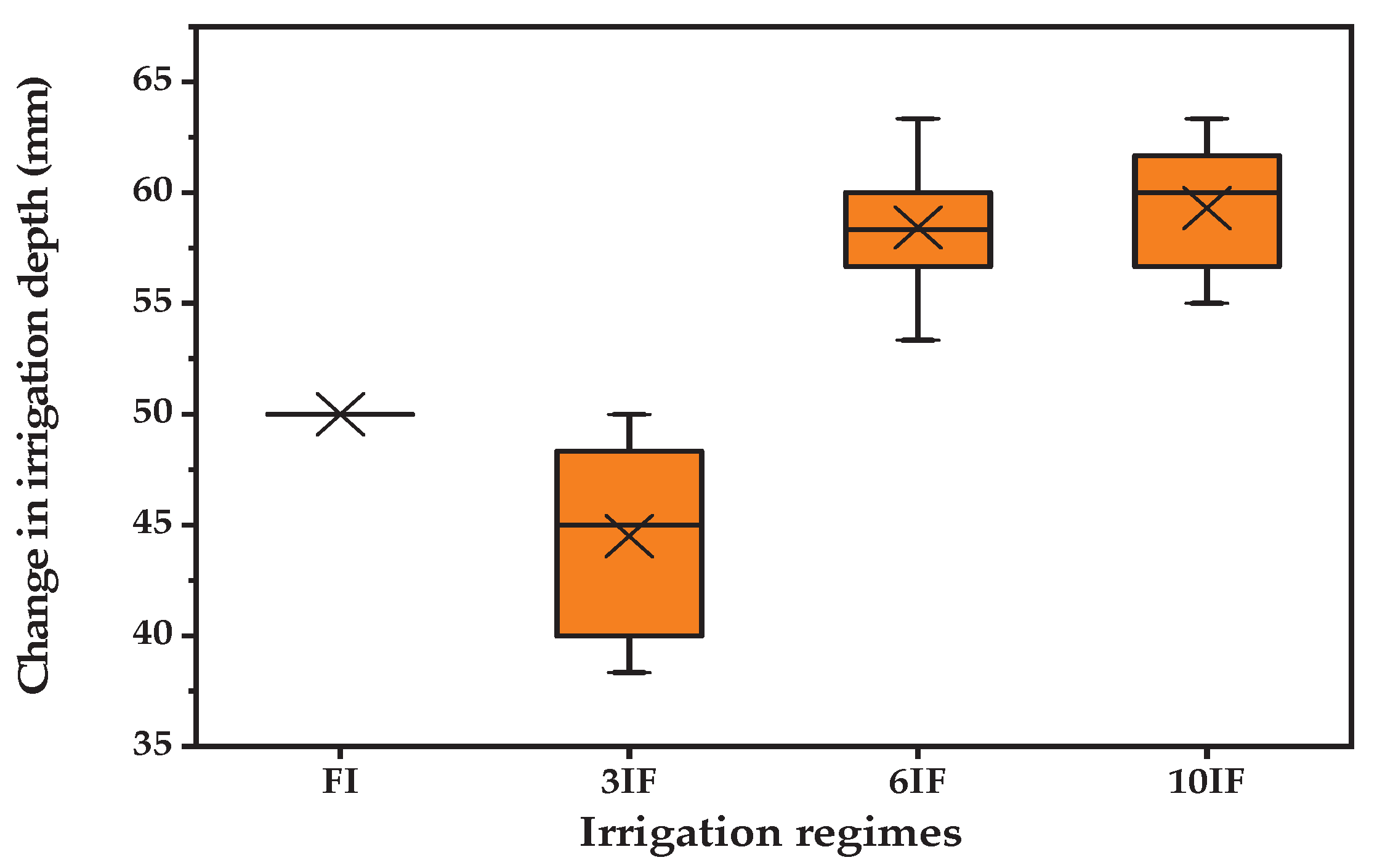
3.1. Results of the In-Field Experiments

The in-field experimental results, including the total irrigation depth, B (t·ha⁻¹), Y (t·ha⁻¹), ET_act (mm), WUE, and WP, for both calibration (2019) and validation (2020) seasons, are listed in

Table 3. Average of total irrigation water, biomass, dry yield, actual evapotranspiration, water use efficiency, water productivity, and harvest index during the growing seasons (2019 and 2020).

Irrigation Regime		Total Irrigation Depth (mm)	Biomass (t·ha−1)	Dry yield (t·ha−1)	ETact (mm)	Percolation (mm)	WUE	WP (kg·m−3)	HI0 (%)
Calibration season (2019)	FI	1800	20.5	9.5	653.6	1067.1	0.36	0.53	47.0
	3IF	1397	21.0	9.8	650.5	807.2	0.47	0.70	47.0
	6IF	1042	19.1	8.9	635.7	446.1	0.61	0.85	47.0
	10IF	709	15.7	7.2	625.5	248.7	0.88	1.02	46.6
Validation Season (2020)	FI	1650	20.6	9.7	567.7	1047.8	0.34	0.59	47.0
	3IF	1347	21.0	9.8	564.6	859.6	0.42	0.73	47.0
	6IF	1012	19.6	9.1	550.5	589.7	0.54	0.90	47.1
	10IF	669	16.3	7.6	540.5	325.4	0.81	1.14	46.9

Notes: Mean values for the four irrigation regimes are presented. FI, flood irrigation; 3IF, 3-day irrigation frequency; 6IF, 6-day irrigation frequency; 10IF, 10-day irrigation frequency. ET_act, WUE, WP, and ${\mathit{HI}}_0$ indicate actual evapotranspiration, water use efficiency, water productivity, and harvest index, respectively.

. The mean irrigation water varied between 1800 (FI, 2019) and 669 mm (10IF, 2020). The total irrigation water decreased significantly under the 3IF, 6IF, and 10IF regimes, respectively, compared with the FI, because the 3IF, 6IF, and 10IF regimes had decreased irrigation intervals. In contrast, the continuous flood irrigation (FI) led to higher losses of irrigation water (Table 3). Our observations are consistent with Borrell et al. [47] and Alhaj Hamoud et al. [48].

The lowest recorded biomass and yield were 15.7 and 7.2 t·ha⁻¹, respectively, under the 10IF regime during 2019. Meanwhile, the highest biomass (21.0 t·ha⁻¹) and yield (9.8 t·ha⁻¹) were recorded under the 3IF regime in 2019 and 2020, respectively. Compared with that under the FI regime, approximately 18.3–22.4% of the total applied irrigation water was saved, with a slight increase in rice yield (1.0–3.2%), under the 3IF regime, while this percentage was 59.4–60.6% under the 10IF regime, albeit with a significant reduction in yield of 21.6–24.2%. The significant increase in rice yield per hectare under the FI regime during 2019 (9.5 t·ha⁻¹) and 2020 (9.7 t·ha⁻¹) compared with that under the other regimes may be due to improvements in grain yield components (e.g., panicle number·m⁻², panicle weight, and 1000 grain weight). Furthermore, these results may be explained by the availability of irrigation water under this irrigation regime, which may enhance production through the conveyance of dry matter to panicles, leading to higher grain filling, weight, and grain yield [49]. Meanwhile, the increase in rice yield per hectare under the 3IF regime may be due to better aeration accompanying higher transformation and absorption of NPK in the soil. These results are consistent with those reported by El-Refaee [49], Ghazy [50], and Ibrahim et al. [51]. Meanwhile, the significant decrease in the observed biomass and yield under the 6IF and 10IF regimes may be due to the reduction in the photosynthetic ratio under water deficit, leading to low productivity [52].

The observed ET_act results reflected its importance in the relevant irrigation regimes, and its effect on crop yield [53], as shown in Table 3. The highest ET_act value was 653.6 mm under the FI regime (Y = 9.5 t·ha⁻¹, 2019). Meanwhile, the lowest ET_act value was 540.5 mm under the FI regime (Y = 7.6 t·ha⁻¹, 2020). Compared with that in the FI regime, there was a slight reduction in the ET_act value by 4.3% and 4.8% under the 10IF regime in 2019 and 2020, respectively. The slight reduction in ET_act under severe irrigation regimes (6IF and 10IF) may be due to the decrease in soil evaporation (E_s) as a result of drying of the soil surface and a decrease in transpiration (T_r). Under such conditions, plants exposed to a severe water deficit tend to close their stomata to preserve their inner moisture content, which further decreases transpiration, photosynthetic rate, and productivity [52]. Accordingly, as a C3 crop, rice can reduce stomatal conductance under water stress, thereby decreasing the total ET_act. The obtained values of ${\mathit{ET}}_{\mathit{act}}$ were similar to those reported by Alberto et al. [54], Maniruzzaman et al. [15], and Xu et al. [55], but lower than those reported by Sudhir-Yadav et al. [56] (749–911 mm) and Moratiel and Martínez-Cob [57] (755–811 mm) for cultivated rice.

Regarding WUE and WP, the lowest WUE values were 0.36 and 0.34 under the FI regime, while the highest values were 0.88 and 0.81 under the 10IF regime during the calibration (2019) and validation (2020) seasons, respectively. Similarly, the lowest WP values were 0.53 and 0.59 kg·m⁻³ under the FI regime, and the highest values were 1.02 and 1.14 kg·m⁻³ under the 10IF regime during 2019 and 2020, respectively. The obtained results were consistent with the report by Ragab [11] that the application of DI strategies in arid regions improved WUE and WP.

Our results illustrated that the 3IF regime was the best among the four examined regimes for achieving the greatest rice biomass and yield. These results were consistent with previous reports on rice under different irrigation regimes in Egypt (e.g., Abou EL Hassan [58]; Tantawi and Ghanem [59]). However, in cases of water scarcity, the slight increase in yield (1.0–3.2%) under the 3IF regime may be diminished to save more irrigation water. Hence, the 6IF regime was an additional viable option for saving about 38.7–42.1% of irrigation water, although it came with a slight reduction in yield (6.2–6.3%). Moreover, usage of such regimes (3IF and 6IF) was suitable for some local varieties, such as Giza 179 [58], Sakha 102, and Sakha 104 [60]. Our findings were consistent with many cited studies, which reported that application of the 3IF and 6IF regimes in rice fields would lead to high grain yields and avoid severe water stress (e.g., Zayed et al. [61], El Refaee et al. [62,63], and Ashouri [64]).

Meanwhile, in the case of severe water scarcity and availability of rice land, the 10IF regime may be the best for achieving the highest WUE and WP, with an increase in mean rice yield from 9.5 t to 18.3 t in 2019 and from 9.8 t to 18.7 t in 2020 using the same amount of applied irrigation water under the FI regime; however, the adoption of this DI strategy requires focusing on the degree of risk of change in irrigation regime at the environmental scale. Changes in saturation conditions affect the emission of greenhouse gases. Flood conditions were considered a minor source of N₂O emissions; however, the effective application of alternative wetting-dry irrigation regimes would decline CH₄ emissions by 70% in rice fields [65]. On the other hand, the irrigation regime affects the percolation rates: the latter has a significant long-term effect on groundwater reserves by increasing or decreasing the amount of recharged water in the deeper layer of soil. Thus, the recharge rate must be considered when planning long-term IF irrigation strategies. In addition, more studies, including those involving varied genotypes and soil types under different ET_act and irrigation regimes, are required to determine the potential differences in degree of risk and efficiency between various IF irrigation regimes [15].

3.2. Calibrated Rice Parameters

The majority of the calibrated rice parameters slightly varied across the four irrigation regimes, whereas the ${\mathit{Kc}}_{\mathit{Tr},\mathit{X}}$ coefficient and ${\mathit{WP}}^{*}$ remained constant. The Ks values varied between 0 and 0.55, reflecting a moderate to extreme sensitivity to water stress under the IF regimes (Table 2). The ${\mathit{CC}}_{\mathit{X}}$ ranged between 91% and 97% under all irrigation regimes, and these values were reached almost at the middle of the flowering stage (Figure 6 and Figure 7). The highest ${\mathit{CC}}_{\mathit{X}}$ value of 97% was reached under the 3IF irrigation regime. Similar results were obtained by Maniruzzaman et al. [15]. Moreover, ${\mathrm{Z}}_{\mathit{X}}$ and ${\mathrm{Z}}_{\mathrm{n}}$ increased with increase in irrigation frequency (IF), whereas the maximum values of, respectively, 0.16 and 0.39 m, were obtained under the 10IF irrigation regime. The obtained results were consistent with those obtained by Elsadek [66], who reported that plants tend to extend their roots in the root zone area to obtain more water and nutrients when irrigation frequencies are increased.

The ${\mathit{WP}}^{*}$ value was set as 19 g·m⁻², which was in the recommended range of 15–20 g·m⁻² for C3 crops, including rice [42]. A similar value of 19 g·m⁻² was obtained by Amiri [67], Maniruzzaman et al. [15], and Raes et al. [25], who modeled rice development stages under full and deficient irrigation conditions using the AquaCrop model. The ${\mathit{HI}}_0$ value was set at 47%, which was in the recommended range (35–50%) for rice [25]. There was a slight variation in the observed ${\mathit{HI}}_0$ values (46.2%–47.2%), which may be because of the randomized in-field variations [15].

3.3. Model Performance Evaluation

3.3.1. Model Performance in Simulating Canopy Cover

Overall, there was a good match between the observed and simulated CC (Figure 6 and Figure 7). The AquaCrop model performance ranged from good to excellent in simulating the CC of rice during the calibration (2019) and validation (2020) seasons (

Table 4. Statistical indicators in estimating canopy, biomass, and actual crop evapotranspiration during 2019 and 2020.

Statistical Indicator		Canopy Cover (%)				Biomass (t·ha−1)				Actual Crop Evapotranspiration (mm)
		FI	3IF	6IF	10IF	FI	3IF	6IF	10IF	FI	3IF	6IF	10IF
Calibration season (2019)	NRMSE	11.6	14.1	9.7	5.9	11.3	11.6	10.3	8.8	12.7	12.6	16.9	32.4
	d	0.98	0.98	0.99	0.99	0.99	0.98	0.99	0.99	0.89	0.89	0.82	0.57
	R2	0.96	0.93	0.98	0.99	0.98	0.99	0.99	0.99	0.65	0.67	0.54	0.28
	EF	0.95	0.93	0.97	0.99	0.98	0.98	0.98	0.99	0.64	0.64	0.46	−0.17
Validation Season (2020)	NRMSE	11.3	15.0	11.7	5.0	14.5	13.2	9.56	7.9	13.8	13.89	16.8	26.8
	d	0.98	0.97	0.99	0.99	0.98	0.99	0.99	0.99	0.83	0.83	0.96	0.61
	R2	0.96	0.92	0.97	0.99	0.99	0.98	0.99	0.99	0.54	0.53	0.43	0.26
	EF	0.95	0.92	0.96	0.99	0.97	0.97	0.98	0.99	0.47	0.45	0.33	−0.07

Notes: Mean values for four irrigation regimes are presented. FI, flood irrigation; 3IF, 3-day irrigation frequency; 6IF, 6-day irrigation frequency; 10IF, 10-day irrigation frequency. NRMSE, d, R², and EF indicate normalized root-mean-squared error, index of agreement, coefficient of determination, and Nash–Sutcliffe efficiency coefficient, respectively. A d value closer to 1 indicates a perfect agreement between the observed and simulated data. NRMSE < 10% is excellent, 10–20% is good, 20–30% is acceptable, and NRMSE > 30% is poor. R² $>$ 0.5 is good. EF < 0 reflects unacceptable performance.

). The average statistical indicators for CC were$5.9\le \mathrm{NRMSE}\le 14.1$. and $5.0\le \mathrm{NRMSE}\le 15.0$; and$0.97\le \mathrm{d}\le 0.99$;$0.93\le {\mathrm{R}}^2\le 0.99$ and$0.92\le {\mathrm{R}}^2\le 0.99$; and $0.93\le \mathrm{EF}\le 0.99$ and $0.92\le \mathrm{EF}\le 0.99$ under the four irrigation regimes during 2019 and 2020, respectively (Table 4).

Figure 6. Observed and simulated average canopy cover during the calibration period (2019) under four irrigation regimes. FI, flood irrigation (a); 3IF, 3-day irrigation frequency (b); 6IF, 6-day irrigation frequency (c); and 10IF, 10-day irrigation frequency (d). Error bars indicate standard deviation among the three replicates.

Figure 6. Observed and simulated average canopy cover during the calibration period (2019) under four irrigation regimes. FI, flood irrigation (a); 3IF, 3-day irrigation frequency (b); 6IF, 6-day irrigation frequency (c); and 10IF, 10-day irrigation frequency (d). Error bars indicate standard deviation among the three replicates.

Figure 7. Observed and simulated average canopy cover during the validation period (2020) under four irrigation regimes. FI, flood irrigation (a); 3IF, 3-day irrigation frequency (b); 6IF, 6-day irrigation frequency (c); and 10IF, 10-day irrigation frequency (d). Error bars indicate standard deviation among the three replicates.

Figure 7. Observed and simulated average canopy cover during the validation period (2020) under four irrigation regimes. FI, flood irrigation (a); 3IF, 3-day irrigation frequency (b); 6IF, 6-day irrigation frequency (c); and 10IF, 10-day irrigation frequency (d). Error bars indicate standard deviation among the three replicates.

The obtained results are consistent with those reported by Maniruzzaman et al. [15] who validated the model under different irrigation regimes in Bangladesh, and by Xu et al. [55] who simulated rice development under wet conditions in China, but superior to those reported by Araya et al. [27], Bello and Walker [68], Du et al. [69], and Iqbal et al. [29]. The obtained results indicated overestimation of CC in days close to ${\mathit{CC}}_{\mathit{X}}$ by AquaCrop, as shown in Figure 6 and Figure 7, consistent with the results reported by Amiri [67], Saadati et al. [70], and Xu et al. [55]. Furthermore, AquaCrop tended to overestimate CC even under severe irrigation regimes in 2019 and 2020, as shown in Figure 6c,d and Figure 7c,d; however, rice is more vulnerable to water stress, which is expected to result in fewer tillers and lower CC than values under a full irrigation regime, owing to the negative effect on rice LAI. These results are consistent with those reported by Xu et al. [55], who showed that AquaCrop may fail to detect the potential effect of water stress on the extension of crop leaves during cultivation.

3.3.2. Model Performance in Simulating Biomass and Yield

Similar to CC, there was a good match between the observed and simulated biomass data (Figure 8 and Figure 9). In addition, the AquaCrop model performance was good to excellent in simulating aboveground biomass and rice yield during the validation and calibration seasons (Table 4). The average statistical indicators for B were$8.8\le \mathrm{NRMSE}\le 11.6$ and $7.9\le \mathrm{NRMSE}\le 14.5$;$0.98\le \mathrm{d}\le 0.99$ and $0.98\le \mathrm{d}\le 0.99$; $0.98\le {\mathrm{R}}^2\le 0.99$ and $0.98\le {\mathrm{R}}^2\le 0.99$; and $0.98\le \mathrm{EF}\le 0.99$ and $0.97\le \mathrm{EF}\le 0.99$ under the four irrigation regimes during 2019 and 2020, respectively (Table 4). There was a slight overestimation of aboveground biomass, ranging between 2.4–4.4% in 2019 and 2.6–4.4% in 2020 (

Table 5. Percent deviation of rice biomass, yield, and in-field water balance components during 2019 and 2020.

Irrigation Regime		Biomass (t·ha−1)			Yield (t·ha−1)			Evapotranspiration (mm)			Percolation (mm)			Change in Soil Water Storage (mm)
		Obs.	Sim.	${\mathbf{P}}_{\mathbf{d}}\left(\%\right)$	Obs.	Sim.	${\mathbf{P}}_{\mathbf{d}}\left(\%\right)$	Obs.	Sim.	${\mathbf{P}}_{\mathbf{d}}\left(\%\right)$	Obs.	Sim.	${\mathbf{P}}_{\mathbf{d}}\left(\%\right)$	Obs.	Sim.
Calibration season (2019)	FI	20.5	21.4	4.4	9.5	10.1	6.3	653.6	630.9	−3.5	1067.1	1125.0	5.4	79.3	44.1
	3IF	21.0	21.5	2.4	9.8	10.2	4.1	650.5	624.2	−4.0	807.2	793.5	−1.7	−60.8	−20.3
	6IF	19.1	19.6	2.6	8.9	9.3	4.5	635.7	593.3	−6.7	446.1	462.3	3.6	−39.8	−13.6
	10IF	15.7	16.2	3.2	7.2	7.5	4.2	625.5	499.4	−20.2	248.7	237.9	−4.3	−165.2	−28.3
Validation Season (2020)	FI	20.6	21.5	4.4	9.7	10.1	4.1	567.7	544.9	−4.0	1047.8	1074.6	2.6	34.5	30.5
	3IF	21.0	21.6	2.9	9.8	10.2	4.1	564.6	540.6	−4.3	859.6	875.8	1.9	−76.9	−69.1
	6IF	19.6	20.1	2.6	9.1	9.5	4.4	550.5	516.3	−6.2	589.7	537.2	−8.9	−128.2	−41.5
	10IF	16.3	16.8	3.1	7.6	7.9	3.9	540.5	460.5	−14.8	325.4	275.7	−15.3	−196.9	−67.2

Notes: Mean values are the means of three replications for each irrigation regime: FI, flood irrigation; 3IF, 3-day irrigation frequency; 6IF, 6-day irrigation frequency; 10IF, 10-day irrigation frequency. Obs. and Sim. refer to the observed and simulated values, and ${\mathrm{P}}_{\mathrm{d}}$ percent deviation (simulation error), respectively. ${\mathrm{P}}_{\mathrm{d}}$ between ±15 is acceptable.

). Similarly, rice yield was slightly overestimated by 4.1–6.3% in 2019 and 3.9–4.4% in 2020 under the four irrigation regimes, as shown in Table 5.

This overestimation of B and Y during the two growing seasons may be due to the underestimation of transpiration, which represents a crucial element in computing biomass and dry yield using the AquaCrop model. Furthermore, the unsuitable division of $E{T}_{act}$ components ($T_r+E_s$) most likely led to the overestimation of crop yield using the AquaCrop model. Similar results have been reported by Adeboye et al. [71] and Nyathi et al. [72]. Our results showed a good correlation between the observed and simulated rice yield, with an R² of 0.99 and 0.98 in 2019 and 2020, respectively (Figure 10a,b). Similar results have been reported by Adeboye et al. [71].

Although many previous studies have reported much greater deviation in simulated yield for many crops, such as maize [31], wheat [29,73], and barley [27] under water stress conditions, in the present study, the overestimation was slight even under severe irrigation regimes during 2019 and 2020 (Table 5). This overestimation may be because the AquaCrop model failed to precisely assess water stress [55]. Our statistical results for aboveground biomass and rice yield were within the range of values reported in several peer-reviewed studies that modeled rice development under full and deficient irrigation conditions using the AquaCrop model (e.g., Maniruzzaman et al. [15], Saadati et al. [70], and Xu et al. [55]).

3.4. Model Performance in Simulating in-Field Water Balance Components

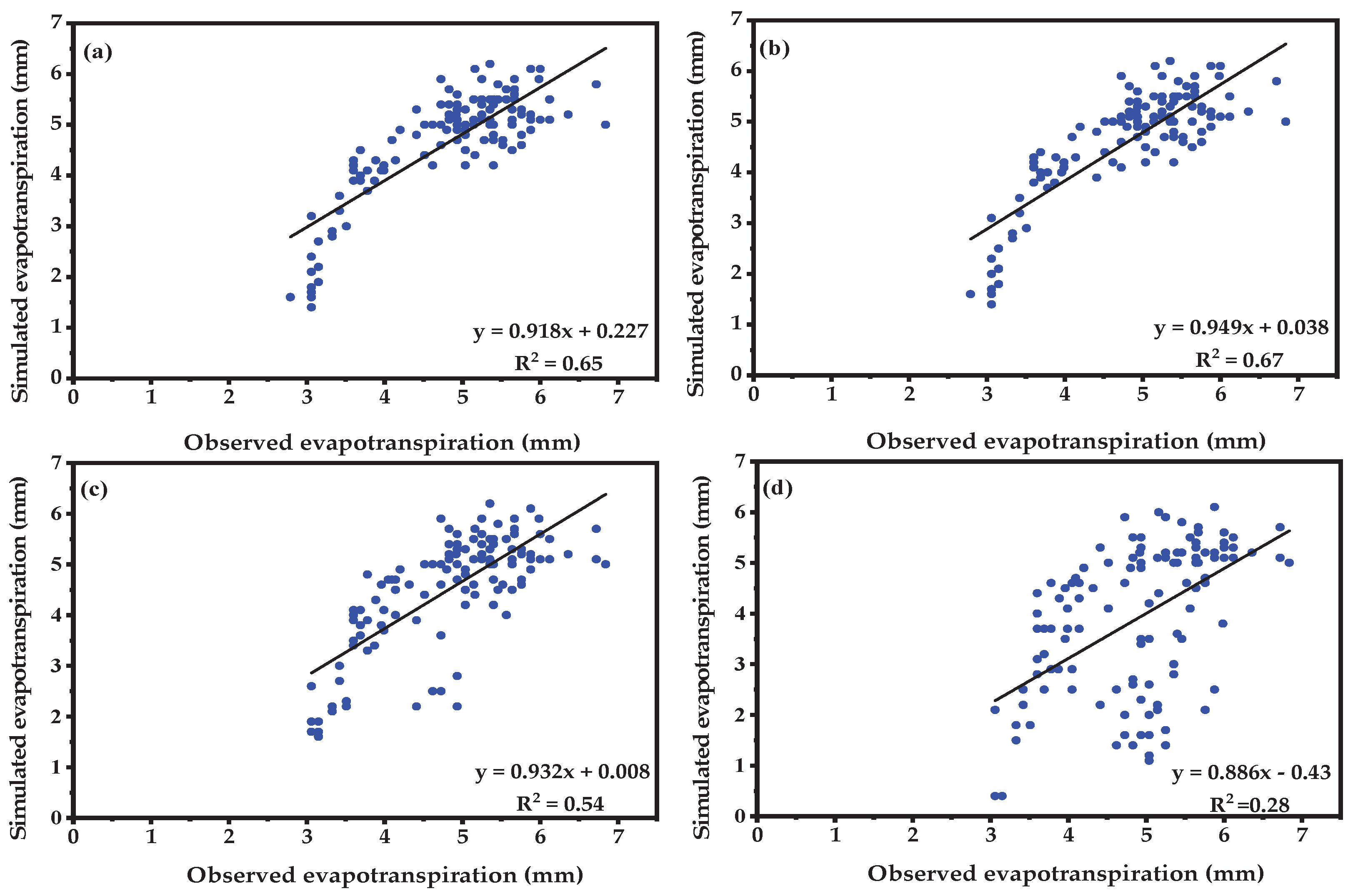
3.4.1. ET_act

Overall, the model performance in simulating ${\mathit{ET}}_{\mathit{act}}$ ranged from good to acceptable under different irrigation regimes during the calibration (2019) and validation (2020) seasons, except under the 10IF regime, in which the model showed poor performance (Table 4 and Table 5). The average statistical indicators for ET_act were 12.6 ≤ NRMSE ≤ 32.4 and 13.8 ≤ NRMSE ≤ 26.8; 0.57 ≤ d ≤ 0.89 and 0.61 ≤ d ≤ 0.96; 0.28 ≤ R² ≤ 0.67 and 0.26 ≤ R² ≤ 0.54; and −0.17 ≤ EF ≤ 0.64 and −0.07 ≤ EF ≤ 0.47 under the four irrigation regimes during 2019 and 2020, respectively (Table 4). The model tended to underestimate ${\mathit{ET}}_{\mathit{act}}$, whereas the range of percent deviation (${\mathrm{P}}_{\mathrm{d}}$) on average was between −3.5% and −20.2% during 2019 and 2020. These deviations were close to or exceeded the recommended ratio of 15% for crop models by Brisson et al. [74], reflecting a good to poor match between the observed and simulated ${\mathit{ET}}_{\mathit{act}}$ under the four irrigation regimes (Table 5). The observed underestimation of ${\mathit{ET}}_{\mathit{act}}$ may be a result of underestimated transpiration due to ${\mathit{Kc}}_{\mathit{Tr},\mathit{X}}$or soil evaporation, resulting in poor predictive performance. Similar high deviations were recorded for ${\mathit{ET}}_{\mathit{act}}$ by Adeboye et al. [71] in soybeans (−20% to 36%), by Farahani et al. [75] in cotton (2.1% to 10.2%), by Heng et al. [76] in maize (−1.23% to −8.4%), and by Maniruzzaman et al. [15] in rice (−15.29% to 10% for separated ${\mathit{ET}}_{\mathit{act}}$) using the AquaCrop model.

Similarly, there was a good to poor correlation between the simulated and observed ${\mathit{ET}}_{\mathit{act}}$ ranging between 0.26 (10IF, 2020) and 0.67 (3FI, 2019), as shown in Figure 11 and Figure 12. It was observed that the model did not simulate ${\mathit{ET}}_{\mathit{act}}$ well under severe water deficit (10IF regime), and there was a weak correlation between the simulated and observed ${\mathit{ET}}_{\mathit{act}}$ (R² = 0.28, 2019 and 0.26, 2020) (Figure 11d and Figure 12d). Moreover, the k-fold_R² values were 0.63 under FI and 0.24 under 10IF. Meanwhile, the k-fold_NRMSE values varied between 13.5% under FI and 30.6% under 10IF, as shown in

Table 6. K-fold cross-validation results (5 folds).

Irrigation Regime	Actual Crop Evapotranspiration (ETact)
	FI	3IF	6IF	10IF
K-foldR2	0.63	0.62	0.51	0.24
K-foldNRMSE	13.5	13.8	17.2	30.6

Notes: Mean values for four irrigation regimes are presented. FI, flood irrigation; 3IF, 3-day irrigation frequency; 6IF, 6-day irrigation frequency; 10IF, 10-day irrigation frequency. R² and NRMSE indicate coefficient of determination and normalized root-mean-squared error, respectively. R²$>$ 0.5 is good. NRMSE < 10% is excellent; 10–20% is good, 20–30% is acceptable, and NRMSE > 30% is poor.

. These k-fold results reflected good to acceptable performance in simulating ET_act under different irrigation regimes, except under the 10IF regime, in which the model showed poor performance.

Based on our analyses, our findings illustrated that AquaCrop had a general tendency to underestimate or overestimate ET_act frequently during the two growing seasons (Figure 11 and Figure 12). Furthermore, we observed that AquaCrop failed to match the ET_act value on the irrigation day. These errors in simulating daily ETact were more evident under the IF regimes, especially 10IF. Under the 10 IF regime, the model showed a significant tendency to underestimate ET_act compared with other regimes, as shown in Figure 11d and Figure 12d. These findings were consistent with those of Sandhu and Irmak [13], who demonstrated that the performance of AquaCrop significantly declined under water stress, and also with those of Katerji et al. [77] for corn and tomato, Montoya et al. [78] for potato, and Xu et al. [55] for rice crops. This underestimation might be due to the errors in calculating the crop coefficient (kc) by AquaCrop. Therefore, the process of calculating ${\mathit{ET}}_{\mathit{act}}$ in Aquacrop must be re-evaluated to obtain a high agreement between the observed and simulated values.

3.4.2. P and ΔS

There were apparent differences between the simulated and observed values of P and ΔS, reflecting the total water required under different irrigation regimes (Table 5). The P rate showed a downward trend under the four irrigation regimes, with the highest values obtained under the FI regime (1067.1 and 1047.8 mm) and the lowest under the10IF regime (248.7 mm and 325.4 mm) during 2019 and 2020, respectively. The highest recorded values of the percolation rate under the FI regime may be explained by the increase in irrigation frequencies, which increased the total amount of irrigation water and, consequently, the total amount of percolation water (Table 5). A similar pattern has been observed by Alhaj Hamoud et al. [48] in rice cultivated in clay soil under different irrigation regimes.

In the present study, the $\mathrm{P}$ rate accounted for, respectively, 35.1%–59.3% and 45.9%–63.5% of the total irrigation water in 2019 and in 2020. The obtained ratio was lower than the reported range (50–80%) for rice fields by Sharma [79]; this may be due to the adoption of DI strategy in the present study, which decreased percolation flows. Moreover, the model simulated more P and less ΔS under the FI regime than under the other irrigation regimes during both calibration and validation seasons (Table 5). A similar pattern has been observed by Maniruzzaman et al. [15].

Overall, based on the ${\mathrm{P}}_{\mathrm{d}}$values, the AquaCrop model showed good to poor performance in simulating the P rates and ΔS. The average percent deviations for the P rate were −4.3 ≤ P_d ≤ 5.4 and −15.3 ≤ P_d ≤ 2.6 under the four irrigation regimes during 2019 and 2020, respectively. The highest percent deviation of −15.3% was recorded under the 10IF regime, reflecting poor model performance in simulating the $\mathrm{P}$ rate under water stress, as reported by Brisson et al. [74]. Similar deviations, ranging between −15.3% and 2.6%, for the P rate using AquaCrop have been reported for rice during the dry season in Bangladesh [15].

4. Conclusions

Here, we examined the in-field water balance of direct-seeded rice (Giza 178 genotype) under various irrigation regimes and arid conditions in Egypt. Four irrigation regimes, namely, continuous flood irrigation with a fixed water depth of 5 cm, and 3-, 6-, and 10-day irrigation frequencies (FI, 3IF, 6IF, and 10IF, respectively), were arranged in a randomized complete block design (RCBD) with three replicates during 2019 and 2020. Then, the feasibility of using AquaCrop (version 6.1) in simulating direct-seeded rice development and in-field water balance was assessed. Our findings demonstrated that both the 3IF and 6IF irrigation regimes were the best for achieving the highest biomass and yield while saving irrigation water, making them the best to apply in Egypt. Meanwhile, in the case of severe water scarcity and rice land availability, the 10IF regime may be the best for achieving the highest WUE and WP, though adopting such irrigation regimes necessitates focusing on the degree of risk associated with changes in irrigation regimes at the environmental scale. Moreover, the AquaCrop model showed excellent performance in simulating canopy cover (CC), biomass (B), and yield (Y), accompanied by a modest but systematized overestimation of these components. However, these slight overestimations lose their significance when the user focuses on relative changes due to changes in irrigation regimes or climate. Further, the model showed acceptable performance in simulating in-field water balance components during the calibration (2019) and validation (2020) seasons, except under the 10IF regime, in which the model performed poorly in simulating actual evapotranspiration (ET_act) and percolation (P). Thus, the process of calculating ${\mathit{ET}}_{\mathit{act}}$ must be re-evaluated to obtain a high degree of agreement between the observed and simulated variables. Considering the potential imperfections in collecting field data, and the robustness of AquaCrop and its performance, our findings highlight the great potential for using this model for irrigation management, crop yield prediction, and even climate change studies under arid climatic conditions in Egypt.

References

1. Heba, E.; Elbehiry, F. Potential Soil Carbon and Nitrogen Sequestration in Future Land Use under Stress of Climate Change and Water Deficiency in Northern Nile Delta, Egypt. Agricultura 2019, 111, 47–66. [Google Scholar] [CrossRef]
2. El-Shahway, A.S.; Mahmoud, M.M.A.; Udeigwe, T.K. Alterations in Soil Chemical Properties Induced by Continuous Rice Cultivation: A Study on the Arid Nile Delta Soils of Egypt. Land Degrad. Develop. 2016, 27, 231–238. [Google Scholar] [CrossRef]
3. Mohammadi, A.; Cowie, A.; Anh Mai, T.L.; de la Rosa, R.A.; Kristiansen, P.; Brandão, M.; Joseph, S. Biochar Use for Climate-Change Mitigation in Rice Cropping Systems. J. Clean. Prod. 2016, 116, 61–70. [Google Scholar] [CrossRef]
4. Zhang, Y.; Wang, Y.; Niu, H. Spatio-Temporal Variations in the Areas Suitable for the Cultivation of Rice and Maize in China under Future Climate Scenarios. Sci. Total Environ. 2017, 601–602, 518–531. [Google Scholar] [CrossRef]
5. Elbasiouny, H.; Elbehiry, F. Rice Production in Egypt: The Challenges of Climate Change and Water Deficiency; Springer International Publishing: New York, NY, USA, 2020; ISBN 978-30-3041-629-4. [Google Scholar]
6. Abd El-Kawy, O.R.; Rød, J.K.; Ismail, H.A.; Suliman, A.S. Land Use and Land Cover Change Detection in the Western Nile Delta of Egypt Using Remote Sensing Data. Appl. Geogr. 2011, 31, 483–494. [Google Scholar] [CrossRef]
7. Mostafa, H.; Fujimoto, N. Water Saving Scenarios for Effective Irrigation Management in Egyptian Rice Cultivation. Ecol. Eng. 2014, 70, 11–15. [Google Scholar] [CrossRef]
8. Rice Research and Training Center (RRTC). National Rice Research Program: Final Results of 2012 Growing Season; The Agricultural Research Center, Rice Research and Training Center: Sakha, Egypt, 2013. [Google Scholar]
9. Ramadan, R. Demand and Supply Challenges of Food Security in Egypt; The Egyptian Center for Economic Studies (ECES), Economic Literature Review: Cairo, Egypt, 2015; Available online: https://eces.org.eg/demand-and-supply-challenges-of-food-security-in-egypt/. (accessed on 4 January 2023).
10. El-Ramady, H.R.; El-Marsafawy, S.M.; Lewis, L.N. Sustainable Agriculture and Climate Changes in Egypt BT. In Sustainable Agriculture Reviews; Lichtfouse, E., Ed.; Springer: Dordrecht, The Netherlands, 2013; Volume 12, pp. 41–95. ISBN 978-94-007-5961-9. [Google Scholar]
11. Ragab, R. A Note on Water Use Efficiency and Water Productivity. Available online: http://www.water4crops.org/water-use-efficiency-water-productivity-terminology/ (accessed on 25 May 2022).
12. Bouman, B.A.M.; Hengsdijk, H.; Hardy, B.; Bindraban, P.S.; Tuong, T.P.; Ladha, J.K. Water-Wise Rice Production. In Proceedings of the International Workshop on Water-Wise Rice Production; International Rice Research Institute, Los Baños, Philippines, 8–11 April 2002. [Google Scholar]
13. Sandhu, R. ; Performance of AquaCrop Model in Simulating Maize Growth, Yield, and Evapotranspiration under Rainfed, Limited and Full Irrigation. Agric. Water Manag. 2019, 223, 105687. [Google Scholar] [CrossRef]
14. Gu, Z.; Qi, Z.; Ma, L.; Gui, D.; Xu, J.; Fang, Q.; Yuan, S.; Feng, G. Development of an Irrigation Scheduling Software Based on Model Predicted Crop Water Stress. Comput. Electron. Agric. 2017, 143, 208–221. [Google Scholar] [CrossRef]
15. Maniruzzaman, M.; Talukder, M.S.U.; Khan, M.H.; Biswas, J.C.; Nemes, A. Validation of the AquaCrop Model for Irrigated Rice Production under Varied Water Regimes in Bangladesh. Agric. Water Manag. 2015, 159, 331–340. [Google Scholar] [CrossRef]
16. Razzaghi, F.; Zhou, Z.; Andersen, M.N.; Plauborg, F. Simulation of Potato Yield in Temperate Condition by the AquaCrop Model. Agric. Water Manag. 2017, 191, 113–123. [Google Scholar] [CrossRef]
17. Linker, R.; Ioslovich, I. Assimilation of Canopy Cover and Biomass Measurements in the Crop Model AquaCrop. Biosyst. Eng. 2017, 162, 57–66. [Google Scholar] [CrossRef]
18. Ojeda, J.J.; Volenec, J.J.; Brouder, S.M.; Caviglia, O.P.; Agnusdei, M.G. Modelling Stover and Grain Yields, and Subsurface Artificial Drainage from Long-Term Corn Rotations Using APSIM. Agric. Water Manag. 2018, 195, 154–171. [Google Scholar] [CrossRef]
19. Singh, P.K.; Singh, K.K.; Bhan, S.C.; Baxla, A.K.; Singh, S.; Rathore, L.S.; Gupta, A. Impact of Projected Climate Change on Rice (Oryza sativa L.) Yield Using CERES-Rice Model in Different Agroclimatic Zones of India. Curr. Sci. 2017, 112, 108. [Google Scholar] [CrossRef]
20. Umair, M.; Shen, Y.; Qi, Y.; Zhang, Y.; Ahmad, A.; Pei, H.; Liu, M. Evaluation of the CropSyst Model during Wheat-Maize Rotations on the North China Plain for Identifying Soil Evaporation Losses. Front. Plant Sci. 2017, 8, 1667. [Google Scholar] [CrossRef] [Green Version]
21. Difonzo, F.V.; Masciopinto, C.; Vurro, M.; Berardi, M. Shooting the Numerical Solution of Moisture Flow Equation with Root Water Uptake Models: A Python Tool. Water Resour. Manag. 2021, 35, 2553–2567. [Google Scholar] [CrossRef]
22. Friedman, S.P.; Communar, G.; Gamliel, A. DIDAS—User-Friendly Software Package for Assisting Drip Irrigation Design and Scheduling. Comput. Electron. Agric. 2016, 120, 36–52. [Google Scholar] [CrossRef]
23. Brunetti, G.; Šimůnek, J.; Bautista, E. A Hybrid Finite Volume-Finite Element Model for the Numerical Analysis of Furrow Irrigation and Fertigation. Comput. Electron. Agric. 2018, 150, 312–327. [Google Scholar] [CrossRef] [Green Version]
24. Raes, D.; Steduto, P.; Hsiao, T.; Fereres, E. AquaCrop—The FAO Crop Model to Simulate Yield Response to Water: II. Main Algorithms and Software Description. Agron. J. 2009, 101, 438–447. [Google Scholar] [CrossRef] [Green Version]
25. Raes, D.; Steduto, P.; Hsiao, T.; Fereres, E. Crop Water Productivity. In Calculation Procedures and Calibration Guidance; AquaCrop Version 5.0; FAO, Land and Water Development Division: Rome, Italy, 2015. [Google Scholar]
26. Steduto, P.; Hsiao, T.C.; Raes, D.; Fereres, E. AquaCrop—The FAO Crop Model to Simulate Yield Response to Water: I. Concepts and Underlying Principles. Agron. J. 2009, 101, 426–437. [Google Scholar] [CrossRef] [Green Version]
27. Araya, A.; Habtu, S.; Hadgu, K.M.; Kebede, A.; Dejene, T. Test of AquaCrop Model in Simulating Biomass and Yield of Water Deficient and Irrigated Barley (Hordeum vulgare). Agric. Water Manag. 2010, 97, 1838–1846. [Google Scholar] [CrossRef]
28. Andarzian, B.; Bannayan, M.; Steduto, P.; Mazraeh, H.; Barati, M.E.; Barati, M.A.; Rahnama, A. Validation and Testing of the AquaCrop Model under Full and Deficit Irrigated Wheat Production in Iran. Agric. Water Manag. 2011, 100, 1–8. [Google Scholar] [CrossRef]
29. Iqbal, M.A.; Shen, Y.; Stricevic, R.; Pei, H.; Sun, H.; Amiri, E.; Penas, A.; del Rio, S. Evaluation of the FAO AquaCrop Model for Winter Wheat on the North China Plain under Deficit Irrigation from Field Experiment to Regional Yield Simulation. Agric. Water Manag. 2014, 135, 61–72. [Google Scholar] [CrossRef]
30. Paredes, P.; Wei, Z.; Liu, Y.; Xu, D.; Xin, Y.; Zhang, B.; Pereira, L.S. Performance Assessment of the FAO AquaCrop Model for Soil Water, Soil Evaporation, Biomass and Yield of Soybeans in North China Plain. Agric. Water Manag. 2015, 152, 57–71. [Google Scholar] [CrossRef] [Green Version]
31. Greaves, G.; Wang, Y.-M. Assessment of FAO AquaCrop Model for Simulating Maize Growth and Productivity under Deficit Irrigation in a Tropical Environment. Water 2016, 8, 557. [Google Scholar] [CrossRef]
32. Stricevic, R.; Cosic, M.; Djurovic, N.; Pejic, B.; Maksimovic, L. Assessment of the FAO AquaCrop Model in the Simulation of Rainfed and Supplementally Irrigated Maize, Sugar Beet and Sunflower. Agric. Water Manag. 2011, 98, 1615–1621. [Google Scholar] [CrossRef]
33. Paredes, P.; Torres, M.O. Parameterization of AquaCrop Model for Vining Pea Biomass and Yield Predictions and Assessing Impacts of Irrigation Strategies Considering Various Sowing Dates. Irrig. Sci. 2017, 35, 27–41. [Google Scholar] [CrossRef]
34. Shalaby, A. Assessment of Urban Sprawl Impact on the Agricultural Land in the Nile Delta of Egypt Using Remote Sensing and Digital Soil Map. Int. J. Environ. Sci. 2012, 1, 253–262. [Google Scholar]
35. Shalaby, A.; Tateishi, R. Remote Sensing and GIS for Mapping and Monitoring Land Cover and Land-Use Changes in the Northwestern Coastal Zone of Egypt. Appl. Geogr. 2007, 27, 28–41. [Google Scholar] [CrossRef]
36. Cabangon, R.J.; Tuong, T.P.; Castillo, E.G.; Bao, L.X.; Lu, G.; Wang, G.; Cui, Y.; Bouman, B.A.M.; Li, Y.; Chen, C.; et al. Effect of Irrigation Method and N-Fertilizer Management on Rice Yield, Water Productivity and Nutrient-Use Efficiencies in Typical Lowland Rice Conditions in China. Paddy Water Environ. 2004, 2, 195–206. [Google Scholar] [CrossRef]
37. Vu, S.H.; Watanabe, H.; Takagi, K. Application of FAO-56 for Evaluating Evapotranspiration in Simulation of Pollutant Runoff from Paddy Rice Field in Japan. Agric. Water Manag. 2005, 76, 195–210. [Google Scholar] [CrossRef]
38. Hsiao, T.C.; Heng, L.; Steduto, P.; Rojas-Lara, B.; Raes, D.; Fereres, E. AquaCrop—The FAO Crop Model to Simulate Yield Response to Water: III. Parameterization and Testing for Maize. Agron. J. 2009, 101, 448–459. [Google Scholar] [CrossRef]
39. Gomez, K.A. Techniques for Field Experiments with Rice; International Rice Research Institute: Los Baños, PH, USA, 1972; p. 46. ISBN 9711040492. [Google Scholar]
40. Molden, D.; Oweis, T.; Steduto, P.; Bindraban, P.; Hanjra, M.A.; Kijne, J. Improving Agricultural Water Productivity: Between Optimism and Caution. Agric. Water Manag. 2010, 97, 528–535. [Google Scholar] [CrossRef]
41. Raes, D.; Steduto, P.; Hsiao, T.; Fereres, E. Crop Water Productivity. In Calculation Procedures and Calibration Guidance; AquaCrop Version 4.0; FAO, Land and Water Development Division: Rome, Italy, 2012. [Google Scholar]
42. Raes, D.; Steduto, P.; Hsiao, T.C.; Fereres, E. Crop Water Productivity. In Calculation Procedures and Calibration Guidance; AquaCrop Version 3.0; FAO, Land and Water Development Division: Rome, Italy, 2009. [Google Scholar]
43. Steduto, P.; Hsiao, T.C.; Fereres, E.; Raes, D. Crop Yield Response to Water; FAO Irrigation and Drainage Paper 66; FAO: Rome, Italy, 2012; ISBN 978-92-510-7274-5. [Google Scholar]
44. Jamieson, P.D.; Porter, J.R.; Wilson, D.R. A Test of the Computer Simulation Model ARCWHEAT1 on Wheat Crops Grown in New Zealand. Field Crops Res. 1991, 27, 337–350. [Google Scholar] [CrossRef]
45. Moriasi, D.N.; Arnold, J.G.; Van Liew, M.W.; Bingner, R.L.; Harmel, R.D.; Veith, T.L. Model Evaluation Guidelines for Systematic Quantification of Accuracy in Watershed Simulations. Trans. ASABE 2007, 50, 885–900. [Google Scholar] [CrossRef]
46. Nash, J.E.; Sutcliffe, J.V. River Flow Forecasting through Conceptual Models Part I—A Discussion of Principles. J. Hydrol. 1970, 10, 282–290. [Google Scholar] [CrossRef]
47. Borrell, A.; Garside, A.; Fukai, S. Improving Efficiency of Water Use for Irrigated Rice in a Semi-Arid Tropical Environment. Field Crops Res. 1997, 52, 231–248. [Google Scholar] [CrossRef]
48. Alhaj Hamoud, Y.; Guo, X.; Wang, Z.; Shaghaleh, H.; Chen, S.; Hassan, A.; Bakour, A. Effects of Irrigation Regime and Soil Clay Content and Their Interaction on the Biological Yield, Nitrogen Uptake and Nitrogen-Use Efficiency of Rice Grown in Southern China. Agric. Water Manag. 2019, 213, 934–946. [Google Scholar] [CrossRef]
49. El-Refaee, I. Effect of Application of Rice Straw Compost and NPK Fertilizers under Some Irrigation Regimes on Grain Yield and Water Productivity of EHR1 Hybrid Rice Cultivar. J. Plant Prod. 2012, 3, 445–462. [Google Scholar] [CrossRef] [Green Version]
50. Ghazy, H.A. Effect of Different Irrigation Treatments and Harvest Time on Hybrid Rice Productivity; Kafrelsheikh University: Kafr El-Sheikh, Egypt, 2010. [Google Scholar]
51. Ibrahim, M.E.; El-Shamarka, S.A.; El-Refaee, I.S.; Ali, O.A.M. Effect of Irrigation Intervals and Organic and Mineral Fertilization Systems on Productivity and Quality of Hybrid Rice. Menoufia J. Plant Prod. 2017, 2, 219–234. [Google Scholar] [CrossRef]
52. Hirayama, M.; Wada, Y.; Nemoto, H. Estimation of Drought Tolerance Based on Leaf Temperature in Upland Rice Breeding. Breed. Sci. 2006, 56, 47–54. [Google Scholar] [CrossRef] [Green Version]
53. Srivastava, A.; Sahoo, B.; Raghuwanshi, N.S.; Singh, R. Evaluation of Variable-Infiltration Capacity Model Evapotranspiration Estimates in a River Basin with Tropical Monsoon-Type Climatology. J. Irrig. Drain. Eng. 2017, 143, 04017028. [Google Scholar] [CrossRef] [Green Version]
54. Alberto, M.C.R.; Wassmann, R.; Hirano, T.; Miyata, A.; Kumar, A.; Padre, A.; Amante, M. CO2/Heat Fluxes in Rice Fields: Comparative Assessment of Flooded and Non-Flooded Fields in the Philippines. Agric. For. Meteorol. 2009, 149, 1737–1750. [Google Scholar] [CrossRef]
55. Xu, J.; Bai, W.; Li, Y.; Wang, H.; Yang, S.; Wei, Z. Modeling Rice Development and Field Water Balance Using AquaCrop Model under Drying-Wetting Cycle Condition in Eastern China. Agric. Water Manag. 2019, 213, 289–297. [Google Scholar] [CrossRef]
56. Sudhir-Yadav; Humphreys, E.; Kukal, S.S.; Gill, G.; Rangarajan, R. Effect of Water Management on Dry Seeded and Puddled Transplanted Rice. Field Crops Res. 2011, 120, 123–132. [Google Scholar] [CrossRef]
57. Moratiel, R.; Martínez-Cob, A. Evapotranspiration and Crop Coefficients of Rice (Oryza sativa L.) under Sprinkler Irrigation in a Semiarid Climate Determined by the Surface Renewal Method. Irrig. Sci. 2013, 31, 411–422. [Google Scholar] [CrossRef] [Green Version]
58. Abou ELHassan, W. Effect of Water Deficit at Critical Physiological Stages of Rice on WUE and Productivity. J. Soil Sci. Agric. Eng. 2017, 8, 115–121. [Google Scholar] [CrossRef]
59. Tantawi, A.; Ghanem, S.A. Water Use Efficiency in Rice Culture. In Future of Water Management for Rice in Mediterranean Climate Areas: Proceedings of the Workshops, Montpellier, France, 5–6 September 1998; CIHEAM: Paris, France, 1999; pp. 39–45. [Google Scholar]
60. Moursi, E.A.; Abdelkhalek, A.A. Water Requirement Components of Some Egyptian Rice Varieties in North Nile Delta. Alex. Sci. Exch. J. Int. Q. J. Sci. Agric. Environ. 2015, 36, 131–140. [Google Scholar] [CrossRef]
61. Zayed, B.A.; Shehata, S.M.A.; Elkhoby, W.M.; Kafaga, E.E.E. Rice and Water Productivity as Affected by Irrigation Intervals and Potassium Splitting under Newly Reclaimed Saline Soil. J. Agric. Res. Kafer Elsheikh Univ. 2007, 33, 807–823. [Google Scholar]
62. El-Refaee, I.S.; El-Ekhtyar, A.M.; El-Gohary, A.A. Improving Rice Productivity under Irrigation Intervals and Nitrogen Fertilizer. In Proceedings of the Second Field Crop Conference, Giza, Egypt, 14–16 October 2008; pp. 333–347. [Google Scholar]
63. El-Refaee, I.S.; Gorgy, R.N.; Metwally, T.F. Response of Some Rice Cultivars to Plant Spacing for Improving Grain Yield and Productivity under Different Irrigation Intervals. Alex. J. Agric. Res. 2012, 57, 1–15. [Google Scholar]
64. Ashouri, M. The Effect of Water Saving Irrigation and Nitrogen Fertilizer on Rice Production in Paddy Fields of Iran. Biochem. Bioinform. 2012, 2, 56–59. [Google Scholar] [CrossRef] [Green Version]
65. Pandey, A.; Mai, V.T.; Vu, D.Q.; Bui, T.P.L.; Mai, T.L.A.; Jensen, L.S.; de Neergaard, A. Organic Matter and Water Management Strategies to Reduce Methane and Nitrous Oxide Emissions from Rice Paddies in Vietnam. Agric. Ecosyst. Environ. 2014, 196, 137–146. [Google Scholar] [CrossRef]
66. Elsadek, E. Use of Automatic Control to Improve the Performance of Field Irrigation Systems; Damietta University: Kafr Saad, Egypt, 2018. [Google Scholar]
67. Amiri, E. Calibration and Testing of the Aquacrop Model for Rice under Water and Nitrogen Management. Commun. Soil Sci. Plant Anal. 2016, 47, 387–403. [Google Scholar] [CrossRef]
68. Bello, Z.A.; Walker, S. Evaluating AquaCrop Model for Simulating Production of Amaranthus (Amaranthus Cruentus) a Leafy Vegetable, under Irrigation and Rainfed Conditions. Agric. For. Meteorol. 2017, 247, 300–310. [Google Scholar] [CrossRef]
69. Du, W.; He, X.; Shamaila, Z.; Zeng, A.; Muller, J. Yield and Biomass Prediction Testing of AquaCrop Model for Winter Wheat. Trans. Chin. Soc. Agric. Mach. 2011, 42, 174–183. [Google Scholar]
70. Saadati, Z.; Pirmoradian, N.; Rezaei, M. Calibration and Evaluation of Aqua Crop Model in Rice Growth Simulation under Different Irrigation Managements. In Proceedings of the International Congress on Irrigation and Drainage, Tehran, Iran, 15–23 October 2011; pp. 589–600. [Google Scholar]
71. Adeboye, O.B.; Schultz, B.; Adekalu, K.O.; Prasad, K.C. Performance Evaluation of AquaCrop in Simulating Soil Water Storage, Yield, and Water Productivity of Rainfed Soybeans (Glycine max L. Merr) in Ile-Ife, Nigeria. Agric. Water Manag. 2019, 213, 1130–1146. [Google Scholar] [CrossRef]
72. Nyathi, M.K.; Van Halsema, G.E.; Annandale, J.G.; Struik, P.C. Calibration and Validation of the AquaCrop Model for Repeatedly Harvested Leafy Vegetables Grown under Different Irrigation Regimes. Agric. Water Manag. 2018, 208, 107–119. [Google Scholar] [CrossRef]
73. Mohammadi, M.; Ghahraman, B.; Davary, K.; Ansari, H.; Shahidi, A.; Bannayan, M. Nested Validation of Aquacrop Model for Simulation of Winter Wheat Grain Yield, Soil Moisture and Salinity Profiles under Simultaneous Salinity and Water Stress. Irrig. Drain. 2016, 65, 112–128. [Google Scholar] [CrossRef]
74. Brisson, N.; Ruget, F.; Gate, P.; Lorgeou, J.; Nicoullaud, B.; Tayot, X.; Plenet, D.; Jeuffroy, M.-H.; Bouthier, A.; Ripoche, D.; et al. STICS: A Generic Model for Simulating Crops and Their Water and Nitrogen Balances. II. Model Validation for Wheat and Maize. Agronomie 2002, 22, 69–92. [Google Scholar] [CrossRef]
75. Farahani, H.J.; Izzi, G.; Oweis, T.Y. Parameterization and Evaluation of the AquaCrop Model for Full and Deficit Irrigated Cotton. Agron. J. 2009, 101, 469–476. [Google Scholar] [CrossRef] [Green Version]
76. Heng, L.K.; Hsiao, T.; Evett, S.; Howell, T.; Steduto, P. Validating the FAO AquaCrop Model for Irrigated and Water Deficient Field Maize. Agron. J. 2009, 101, 488–498. [Google Scholar] [CrossRef] [Green Version]
77. Katerji, N.; Campi, P.; Mastrorilli, M. Productivity, Evapotranspiration, and Water Use Efficiency of Corn and Tomato Crops Simulated by AquaCrop under Contrasting Water Stress Conditions in the Mediterranean Region. Agric. Water Manag. 2013, 130, 14–26. [Google Scholar] [CrossRef]
78. Montoya, F.; Camargo, D.; Ortega, J.F.; Córcoles, J.I.; Domínguez, A. Evaluation of Aquacrop Model for a Potato Crop under Differentirrigation Conditions. Agric. Water Manag. 2015, 164, 267–280. [Google Scholar] [CrossRef]
79. Sharma, P.K. Effect of Periodic Moisture Stress on Water-Use Efficiency in Wetland Rice. Oryza 1989, 26, 252–257. [Google Scholar]
Figure 1. Geographic locations and distribution of rice cultivation regions over the study area at a 10 m resolution.
Agronomy 13 00609 g001
Figure 2. General methodological framework of the present study.
Agronomy 13 00609 g002
Figure 3. Change in irrigation depth during the growing seasons of 2019 and 2020 under four irrigation regimes. FI indicates flood irrigation, and 3IF, 6IF, and 10IF indicate 3-day, 6-day, and 10-day irrigation frequencies, respectively. The cross and line within the box mark the median and average, respectively; whiskers above and below the box indicate the maximum and minimum irrigation depth during the growing seasons, respectively.
Agronomy 13 00609 g003
Figure 4. Daily temperature and reference evapotranspiration patterns during the growing seasons of (a) 2019 and (b) 2020. Tmax, Tmin, and Tave indicate the maximum, minimum, and average temperature, respectively.
Agronomy 13 00609 g004
Figure 5. Experimental plot set up. (a) Crop evapotranspiration (b) Crop evapotranspiration plus Percolation rate.
Agronomy 13 00609 g005
Figure 8. Observed and simulated average biomass during the calibration period (2019) under four irrigation regimes. FI, flood irrigation (a); 3IF, 3-day irrigation frequency (b); 6IF, 6-day irrigation frequency (c); and 10IF, 10-day irrigation frequency (d). Error bars indicate standard deviation among the three replicates.
Agronomy 13 00609 g008
Figure 9. Observed and simulated average biomass during the validation period (2020) under four irrigation regimes. FI, flood irrigation (a); 3IF, 3-day irrigation frequency (b); 6IF, 6-day irrigation frequency (c); and 10IF, 10-day irrigation frequency (d). Error bars indicate standard deviation among the three replicates.
Agronomy 13 00609 g009
Figure 10. Observed and simulated rice yield during (a) 2019 and (b) 2020 under four irrigation regimes. The correlation (R2) between the observed (x) and simulated (y) yield is considered good (R2 > 0.5). Error bars indicate standard deviation among the three replicates.
Agronomy 13 00609 g010
Figure 11. Observed and simulated crop evapotranspiration during the calibration period (2019) under four irrigation regimes. FI, flood irrigation (a); 3IF, 3-day irrigation frequency (b); 6IF, 6-day irrigation frequency (c); and 10IF, 10-day irrigation frequency (d). The correlation (R2) between the simulated (y) and observed (x) crop evapotranspiration is considered good (R2 > 0.5).
Agronomy 13 00609 g011
Figure 12. Observed and simulated crop evapotranspiration during the validation period (2020) under four irrigation regimes. FI, flood irrigation (a); 3IF, 3-day irrigation frequency (b); 6IF, 6-day irrigation frequency (c); and 10IF, 10-day irrigation frequency (d). The correlation (R2) between the simulated (y) and observed (x) crop evapotranspiration is considered good (R2 > 0.5).
Agronomy 13 00609 g012