Article

Early-Season Mapping of Johnsongrass (Sorghum halepense), Common Cocklebur (Xanthium strumarium) and Velvetleaf (Abutilon theophrasti) in Corn Fields Using Airborne Hyperspectral Imagery

by
María Pilar Martín
1,*,
Bernarda Ponce
1,2,
Pilar Echavarría
1,
José Dorado
3 and
Cesar Fernández-Quintanilla
3
1
Environmental Remote Sensing and Spectroscopy Laboratory (SpecLab), IEGD, Spanish National Research Council (CSIC), Albasanz 27-28, 28037 Madrid, Spain
2
Geotig, Alemania Av. 0999, Office 806, Paseo de Las Artes Building, Temuco 4800885, Chile
3
Institute of Agricultural Sciences (ICA), Spanish National Research Council (CSIC), Serrano 115B, 28006 Madrid, Spain
*
Author to whom correspondence should be addressed.
Agronomy 2023, 13(2), 528; https://doi.org/10.3390/agronomy13020528
Submission received: 9 January 2023 / Revised: 6 February 2023 / Accepted: 9 February 2023 / Published: 11 February 2023
(This article belongs to the Special Issue Advances in Field Spectroscopy in Agriculture)

Abstract

:
Accurate information on the spatial distribution of weeds is the key to effective site-specific weed management and the efficient and sustainable use of weed control measures. This work focuses on the early detection of johnsongrass, common cocklebur and velvetleaf present in a corn field using high resolution airborne hyperspectral imagery acquired when corn plants were in a four to six leaf growth stage. Following the appropriate radiometric and geometric corrections, two supervised classification techniques, such as spectral angle mapper (SAM) and spectral mixture analysis (SMA) were applied. Two different procedures were compared for endmember selections: field spectral measurements and automatic methods to identify pure pixels in the image. Maps for both, overall weeds and for each of the three weed species, were obtained with the different classification methods and endmember sources. The best results were achieved by defining the endmembers through spectral information collected with a field spectroradiometer. Overall accuracies ranged between 60% and 80% using SAM for maps that do not differentiate the weed species while it decreased to 52% when the three weed species were individually classified. In this case, the SMA classification technique clearly improved the SAM results. The proposed methodology shows it to be a promising prospect to be applicable to low cost images acquired by the new generation of hyperspectral sensors onboard unmanned aerial vehicles (UAVs).

1. Introduction

The expansion of geospatial technologies, information and communication technologies, new sensors and precision farming machinery has opened the possibility of adapting crop and pest management to fit the spatial variability conditions found within agricultural fields. Site-specific weed management is the application of this concept to one particular aspect of crop protection: weed control. This site-specific management is based on the fact that weed populations are commonly unevenly distributed in patches within crop fields, which enables applying chemical and/or physical weed control actions only where and when they are really needed [1,2].
Any site-specific weed management program demands accurate weed monitoring. This can be achieved in two different approaches: (a) generation of field weed maps, using them as predictive information in succeeding control operations; (b) real-time weed detection by integrating the sensor and the actuation system [3]. Spatial explicit information on weed distribution may be acquired from image sensors installed either on the ground or aerial platforms. The benefits and limitations of both approaches have been extensively reviewed by Fernández-Quintanilla et al. [4], Gerhards et al. [5], Lati et al. [6] and Lopez-Granados [7]. The ground-based approach typically produces high resolution images, allowing an early detection of relatively low weed densities and discrimination of the major weed species [8,9,10], but operational implementation is limited due to technological constraints and excessive operating costs. Sensors placed on satellites or aerial platforms allow larger areas to be inspected, but image spatial resolution is usually lower [11,12], which challenges the identification of small or low density patches, especially for early (seedling) weed detection. Airborne digital imaging systems have been extensively used in the United States and Australia from late 90s, to map weeds on rangelands, crop residue and seedling crops [13]. Most of these early studies were based in multi-spectral sensors using supervised classification methods, which demand a prior knowledge on the location of representative weed and non-weed sites in the image to train the processor to discriminate those two categories. Additional factors limiting the accuracy of airborne high resolution imaging systems in weed mapping were identified in those pioneer studies, such as the mixed pixels or the lack of essential information linking relevant remote sensing parameters, such as leaf area index and percentage plant coverage, to key management parameters, (e.g. plant density or weed typology) [14]. An alternative to satellite and airborne systems that contributes to lessen or even solve the mixed-pixel problem is the use of unmanned aerial vehicles (UAVs). These platforms can fly at low altitudes, which increase the spatial resolution of the images. Peña et al. [15] and de Castro et al. [16] were able to generate weed maps in early corn, sunflower and cotton crops by combining ultra-high spatial resolution multispectral images obtained from UAVs and an entirely automatic object-based image analysis (OBIA). The main weakness of UAV systems applied to weed monitoring is that they usually carry multispectral sensors, able to obtain information in a reduced number of spectral bands (usually 3 to 5). This can limit the discrimination ability, especially in early growth stages when spectral differences between crops and weeds are small and there is a strong influence from the soil background. The maximum potential for weed identification using UAV platforms relies on the use of image-based machine learning techniques applied to hyperspectral data combining appropriate spatial, spectral and temporal resolutions. Some analyses have revealed the potential of hyperspectral data for this application, using ground or lab-based spectroradiometers [17,18,19] and cameras [20,21,22]. However, a robust and operational implementation of these methods to hyperspectral images acquired from airborne systems or UAVs is still in progress [23].
The use of hyperspectral sensors offers the possibility to improve the accuracy of weed detection and species discrimination. Zhang et al. [12] used a ground hyperspectral image-based plant recognition system to discriminate various weed species from tomato plants in an early growth stage. Aerial detection of late-season weed infestation can offer good results when there is no strong soil background influence, the weeds exceed the crop canopy, and there are quantifiable spectral differences between crops and weeds [7]. Late-season maps can be used in combination with population dynamics knowledge to estimate future weed distribution and to define long-term management plans [24,25]. However, in order to make in-season weed control decisions, it is desirable to detect weed populations at an early growth stage of the crop. Although various studies have shown the possibilities of creating early-season weed maps through multispectral airborne imagery, in many cases, the accuracy of these maps was not as high as desirable [26,27]. Airborne platforms allow using, not only multispectral, but also hyperspectral sensors able to acquire information in hundreds of bands in different spectral regions (from visible to thermal infrared). A number of such systems are currently available, including: the airborne hyperspectral imaging AisaFENIX 1K (Specim, Spectral Imaging Ltd., Oulu, Finland), with up to 620 bands from 380 to 2500 nm; the airborne visible infrared imaging spectrometer (AVIRIS) and next generation (AVIRIS-NG), with 224 bands covering from 400 to 2500 nm [28]; the airborne hyperspectral scanner AHS (ArgonST, Fairfax, VA, USA) with 80 bands covering from 450 nm to 1280 nm; the HySpex imaging spectrometers (Norsk Elektro Optikk AS, Oslo, Norway) with different band configurations, including the visible (VIS), near infrared (NIR) and shortwave infrared (SWIR) spectral domains; the HyMap imaging spectrometer (Integrated Spectronics Inc., Sydney, Australia) which provides 128 bands across the reflective solar wavelength region from 450 to 2450 nm; the APEX airborne prism experiment, an imaging spectrometer developed by a Swiss-Belgian consortium, on behalf of the European Space Agency (ESA) [29], which acquires information in 300 bands in the wavelength range between 400 nm and 2500 nm and is being used as a simulator for the calibration and validation of future spaceborne hyperspectral imagers; and the hyperspectral all-in-one compact airborne spectral imager CASI 1500H (Itres Research Limited, Calgary, AB, Canada) with up to 288 bands in the VIS-NIR spectral region. The CASI imager has been used for early-season aerial weed detection in corn fields by Goel et al. [30] and Karimi et al. [31], while Yang and Everitt [32] used a CCD camera-based hyperspectral imaging system on board a Cessna 404 twin-engine aircraft to map two terrestrial weeds and one aquatic weed. Nowadays, with advances in UAV technologies and their cost-effectiveness, these unmanned vehicles are often preferred to manned aerial platforms [33]. A wide range of new mini-sized and low-cost hyperspectral cameras that can be mounted in UAVs have been developed in the last years and are available for commercial use, generating unprecedented opportunities for weed monitoring combining very high spatial and spectral resolutions.
A number of classification techniques can be used to analyze hyperspectral images, including supervised and unsupervised classifiers [34]. Supervised classification requires a prior knowledge and only known categories are used to train the classifier. Spectral angle mapper (SAM) is a supervised method that admits very quick classification using the spectral angle information derived from the image and reference spectra. Vyas et al. [35] used the SAM to discriminate tropical vegetation and Kumar et al. [36] combined the SAM and spectral information divergence (SID) models to discriminate different species of the same plant genus. They found that this hybrid approach resulted in a better discriminator than the SAM or SID on their own. In agriculture applications, the SAM has been successfully used to map the spatial and temporal dynamics of tillage practices over broad geographic areas [37]. Spectral mixture analysis (SMA) is another supervised classification technique that can be used for both, multi and hyperspectral images [38]. The spectral mapping/unmixing technique can be used as a potential way to solve the challenge of classifying mixed pixels, as they consist of the spectral response of different materials at different proportions. This problem is common in heterogeneous landscapes as urban areas but it is also the case of infested fields where pixels can easily include crops, weeds and soil covers. Miao et al. [39] used images obtained with a CASI sensor and classified by SMA for early mapping of yellow star-thistle (Centaurea solstitialis) infesting California‘s grasslands. Uncertainty of the unmixing results was estimated using a Monte-Carlo approach. The low density of yellow star-thistle (<10%) was well estimated and the uncertainty was less than 4%.
In spite of the unprecedented availability of remote sensing data with potential application in site-specific weed management, the operational use of very high spatial and spectral resolution images obtained from airborne or UAV platforms still require addressing key questions related with: (a) the instrumentation (e.g., platform stability, sensor integration and payload problems); (b) the image quality (e.g., radiometric calibration, geometric distortions); and (c) the processing techniques for image information extraction, including spectral, spatial and temporal analysis algorithms and processing workflows [33]. Further research is needed to quantify the sensitivity of hyperspectral remote-sensing systems for detecting and mapping weeds in terms of weed biomass or density, as well as to better understand the suitable relations between weed species, patch size/density and image spectral/spatial resolution to derive truly operational herbicide prescription maps. In this context, the main objective of this study was to explore the use of AHS airborne hyperspectral scanner as a tool for the early-season mapping of some of the major weed species present in corn crops: johnsongrass, common cocklebur and velvetleaf. These species have been reported as troublesome weeds in corn fields in Central Spain [40] and in extensive corn growing areas of the USA [41]. Previous studies have shown that these three species were present following aggregated distributions [25,40,42]; consequently, we can hypothesize that they are appropriate targets for site-specific weed management. Two different supervised classification techniques, SAM and SMA, were compared and the complementary use of ground spectral information was explored in order to evaluate the potential of high spatial and spectral resolution images to produce general (presence/absence of weeds), as well as species-specific weed maps with the appropriate spatial and temporal characteristics required in site specific management.

2. Materials and Methods

2.1. Study Area

The study was conducted on a 5.2 ha (520 m by 100 m) field at the CSIC experimental farm “La Poveda” located in Arganda del Rey, Madrid, Spain (40.31° N, 3.49° W). Corn (cv. Helen) was planted on 1 April 2007 with 0.75 m row spacing and a population of 85,000 plants ha−1. Corn had been grown continuously during the previous nine years in the eastern half of the field, using conventional tillage and sprinkler irrigation. In the other half, in the three years prior to corn, the field was sown with barley. Although the field received a pre-emergence herbicide treatment with S-metolachlor (1.20 kg a.i. ha−1) + mesotrione (0.12 kg a.i. ha−1), relatively high weed populations of johnsongrass, common cocklebur and velvetleaf were established in different areas of the field.

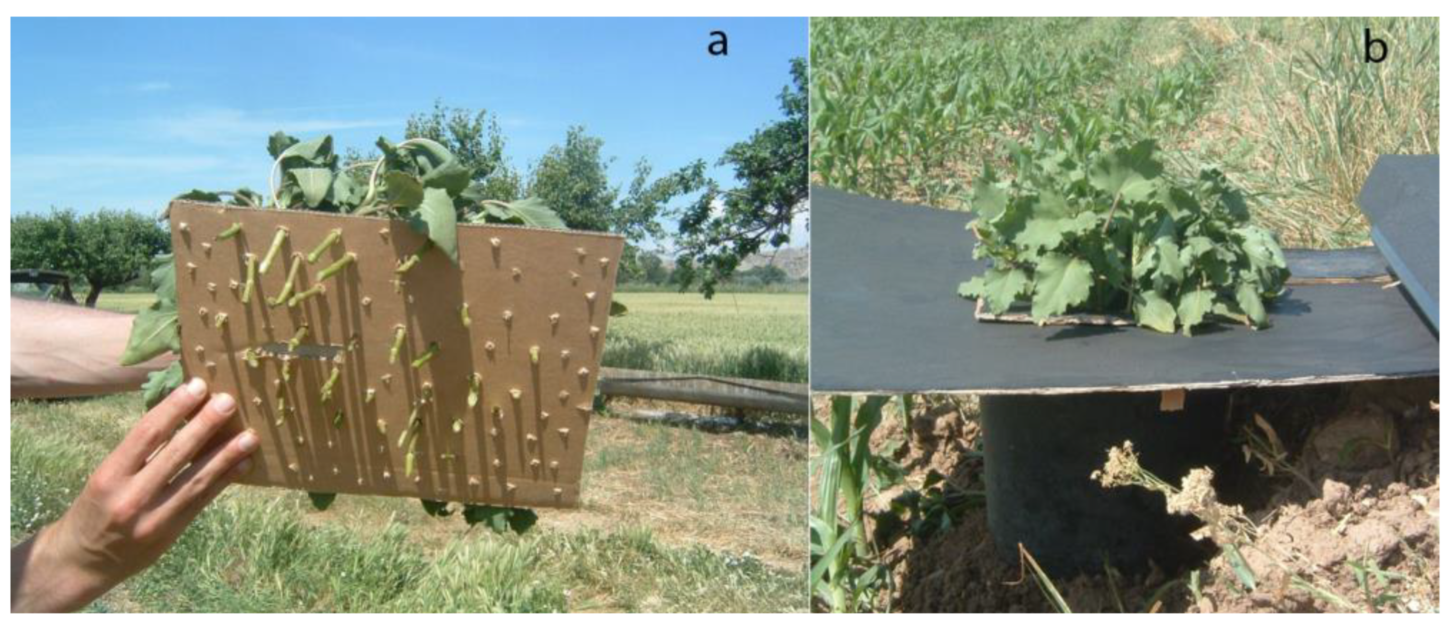
2.2. Data Acquisition: Hyperspectral Images and Ancillary Ground Information

An airborne campaign was conducted over the experimental field on 18 May 2007 using an airborne hyperspectral scanner (AHS) flown onboard a C-212-200 RS aircraft (CASA, Getafe, Spain). The AHS is an 80 bands hyperspectral optical-thermal sensor operated by the National Institute of Aerospace Technology (INTA) as a service to public institutions and private companies for scientific and commercial applications. It is a linescanner with an instantaneous field of view (IFOV) of 2.5 mrad and a total field of view (FOV) of 90°. The AHS records incoming radiation in five optical ports (Table 1). For each of the ports, a grating disperses the radiation and a secondary optical assembly focuses it onto an array of detectors, which defines the final set of (contiguous) spectral bands [43]. In this study, only optical data acquired by ports 1 and 2/2A in the VIS, NIR and SWIR spectral regions were used.
The flight date were selected with the purpose of temporarily matching with the optimal period for the application of herbicides, which would demonstrate the ability of these images to discriminate weed patches at the most appropriate time for operational use of this technology. In order to obtain the best spatial detail, flight altitude was set to 1000 m above ground level which allowed for obtaining images with the sensor’s maximum spatial resolution of 2 m. Image was acquired at 11:30 UTC and flight configuration followed the solar plane in order to minimize the effect of shadows in canopy reflectance.
Simultaneous to the image acquisition, field measurements were performed using an ASD Fieldspec3 FR portable field spectroradiometer (ASD Inc., Boulder, CO, USA) on invariant surfaces (bare soil, asphalt and different fabrics and plastic) to support the image radiometric calibration. This instrument measures the hemispherical-conical reflectance factor (HCRF) from 350 to 2500 nm. The ASD was handled using bare fiber with a nominal FOV of 25°. Spectra were acquired at an approximate height of 1.2 m, rendering a sensor footprint diameter of about 53 cm.
Spectral signatures of the target covers were also measured in-situ using a GER2600 field portable spectroradiometer (Spectra Vista Corporation, Poughkeepsie, NY, USA) with 350 nm to 2500 nm spectral range and 3° FOV. The radiometer was mounted on a tripod to ensure nadiral observations in all measurements. This configuration meant that there was a drawback when trying to move the instrument in the field to the different weed patches. Since the measurements need to be performed in a short period of time to ensure homogeneity in the illumination conditions, we decided on an alternative method to measure quickly and easily the different weed species in the field. The method consisted in placing the spectroradiometer within the field, in the nearest area to several weed patches. There, we fixed the instrument on the tripod at a height of 177 cm, which generated an elliptical FOV of about 30 cm × 24 cm. Plants from the three selected (most abundant) weed species (johnsongrass, common cocklebur and velvetleaf) were collected and located in the area observed by the spectroradiometer. To avoid the influence of ground reflectance in the measured spectral signal, the plants were placed on a tray covered with black paper which was probed to have a high absorbance (>98%) in the full spectral range covered by the spectroradiometer. To simulate as much as possible the actual geometry of a dense and homogeneous cover, each plant was collected keeping the stem, which served to hold them in the black tray, as shown in Figure 1. Similar methodology has been used by other authors [44] to characterize the spectral behavior of individual species at canopy level but simplifying natural field conditions, especially in the context of grasslands and forb systems where relatively small plants dominate the ecosystem.
In order to obtain a good spectral characterization of the weed species, between 10 and 20 spectra per species were acquired. Bare soil spectra were also obtained to characterize the spectral behavior of this background cover. This information was used to define the reference spectral signatures or endmembers required in classification algorithms applied to the AHS image.

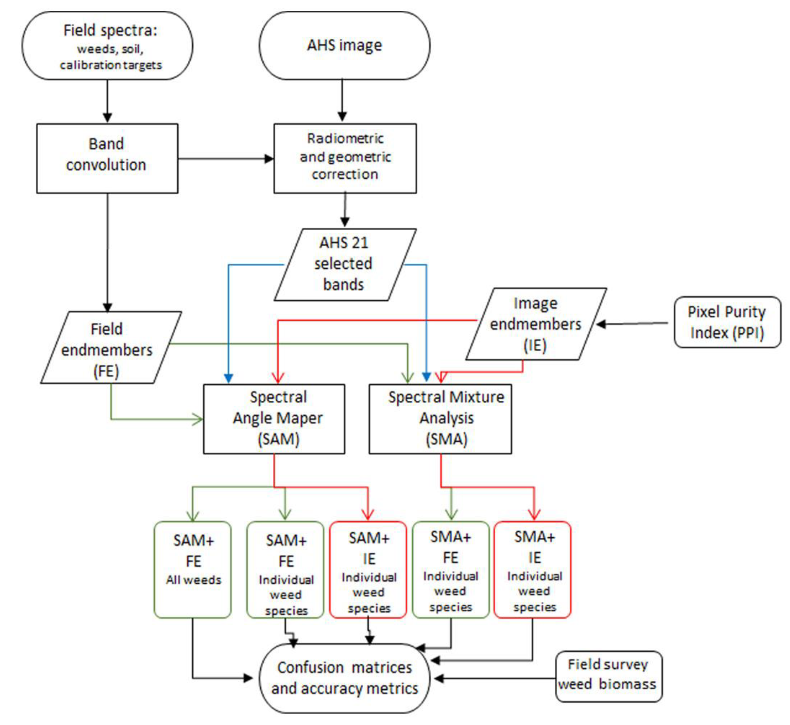
2.3. Hyperspectral Image Pre-Processing

Different AHS image products are available to the users according to their processing level. In this study we used L2c products, which include geometric and radiometric corrections. In L2c images, the radiometric calibration applied transforms the pixel values from digital numbers to at-sensor radiance (Ls). This is further converted to the hemispherical-directional reflectance factor (HDRF) using ATCOR®4 (ReSe Applications Schläpfer, Langeggweg, Switzerland), a look up table-based implementation of MODTRAN®5 (Spectral Sciences, Inc., Burlington, MA, USA, and the U.S. Air Force Research Laboratory, Dayton, OH, USA), an atmospheric radiative transfer model for airborne scanner data. A complete description of the calibration of the AHS bands and the radiometric and atmospheric correction methods applied by INTA can be found in [43].
The HDRF calculated by ATCOR®4 is susceptible to deviations between the real and modeled atmosphere used as reference, calibration errors or the presence of cirrus clouds and contrails in the sky. In order to minimize these problems, an empirical line (EL) correction was used to force image data to match selected field reflectance spectra. This correction was applied to ATCOR®4 output HRDF using a linear regression between the AHS and field spectra measured on invariant surfaces with the ASD Fieldspec3 FR simultaneously with the image acquisition. Some studies suggested that the application of EL to model-based corrected data was much more effective than applying it to the original radiance [45]. This method allows for assessing a priori homogeneity of the surfaces used in terms of reflectance and a more direct comparison with the field spectra.
Image geolocation was performed using the direct georeferencing code PARGE® (ReSe Applications Schläpfer, Langeggweg, Switzerland). It performs an ortho-rectification of line scanner imagery using a digital elevation model (DEM), on the basis of high precision flight parameters, such as global positioning system (GPS) location and attitude angles. In this case, a high resolution 5 m DEM provided by the Spanish National Geographic Institute (IGN) was used. The output geometry file reports the geographic (ETRS89 UTM) easting and northing values derived by the geolocation process for each original image pixel. A nearest neighborhood resampling algorithm was applied to extrapolate pixel values from the image to the UTM coordinates. For a flat terrain, it is assumed that the accuracy obtained with this correction is better than one pixel without using control points. To confirm this, the geometric accuracy was evaluated using orthophotographs at a 0.25 m pixel size provided by the Spanish National Plan of Aerial Photography (PNOA) as a reference. Up to ten control points were located both in the AHS and reference images and the root mean square error (RMSE) was calculated.
A final step in the pre-processing chain consisted in a radiometric quality check in order to detect and remove potential noisy bands due to instrumental problems. Spectral profiles for selected pixels located in homogenous covers as water and asphalt were produced and those bands exhibiting anomalous spectral behavior were discarded for further analysis.

2.4. Image Classification: Weed Maps

Airborne hyperspectral sensors allow for obtaining comprehensive information on the Earth’s surface due to its high spectral resolution. This makes them very suitable in applications requiring discrimination between covers/objects having very similar spectral behavior (e.g., in the differentiation of plant species). Paradoxically, the high spectral dimensionality of these sensors can also result in a degradation of the classification accuracy as a result of the “curse of dimensionality”, that can lead to an overfitting of the training data [46]. Trying to overcome this problem, new spatial and spectral classification schemes have been proposed to be specifically applied to hyperspectral remote sensing data [47]. These algorithms need to solve two major obstacles: spectral variability and background interference. The first one is related to the spectral behavior of the target cover. Unfortunately, variabilities in material composition, atmospheric interferences and sensor noise, introduce random variations in the spectral signature of the different covers which hinder its detection and identification. Moreover, even in high spatial resolution images, measured spectra generally include a mixture of different covers/objects at a pixel level which also complicate their discrimination.
In this work, we have tested the performance of two different supervised classifiers commonly applied to hyperspectral images. A workflow diagram in Figure 2 provides a graphic overview of the process. Both classifiers are popular spectral matching algorithms that use different error metrics and constraints to determine the existence of a spectral similarity between each image pixel spectrum and a set of known/reference “pure” spectra. They have been used in a wide range of applications, including mineral identification [48], monitoring land cover change [49], estimation of fractional vegetation cover [50] and mapping agricultural tillage practices [37], among others. The first method applied is the SAM, a physically-based spectral classification algorithm that calculates the angular distance between spectral signatures of image pixels and training spectral signatures, assuming that they are vectors in an n-dimensional space where n is the number of available bands [51]. One of the main advantages of this method is that it is reasonably insensitive to illumination conditions since the angle between the vectors is independent of its length.
The second algorithm, commonly referred in the literature as SMA, is based on the linear spectral mixture model [52]. This technique has been used to derive subpixel vegetation information, both for multi and hyperspectral images. SMA assumes that the scene is composed of a few fundamental components, or endmembers, each of which is spectrally distinctive from the others. It allows for calculating, in a mixed pixel, the proportion occupied by each component, according to their characteristic spectral behavior. The hypothesis of a linear relationship to explain the meaning of reflectance values in mixed pixels is the most accepted so far. Contrary to what happens in classical classification methods, which generate a single image where each pixel has a code that identifies it as belonging to a particular category, the SMA offers as many images as categories to discriminate. In these images, every pixel is assigned a value representing the percentage of the area occupied by each category.
A common problem to SAM and SMA spectral matching algorithms is to correctly identify the reference spectral signatures of those elements/covers we want to identify in the image, i.e., characteristic spectral values of the endmembers. The term pure member or endmember, commonly used in studies of geochemistry, has been adopted here to designate the spectral response that ideally presents, in the absence of noise, a completely pure pixel, one in which 100% of its area is occupied by only one cover type. These endmembers are of great importance because classification accuracy largely depends on its correct definition. Several methods have been proposed in the literature to define the pure image members or reference spectral signatures for the target covers. In some cases spectral measurements performed in the laboratory or the field are used; in others, the pure pixels are identified in the same image using automatic methods that can be supported by auxiliary information (maps or images of higher spatial resolution). In this study, we tested both approaches in order to analyze their performance by using the spectral signatures of the target covers measured in-situ using a GER2600 field portable spectroradiometer and also with an endmember extraction algorithm applied for finding pure signatures in the AHS image. For the latter, we selected the pixel purity index (PPI), a widely used algorithm implemented in ENVI® 5.1 image analysis software (L3Harris Geospatial Solutions, Inc.). It searches for a set of vertices of a convex hull which are supposed to be pure signatures present in the image [53]. The PPI is computed by repeatedly projecting n-D scatter plots on a random unit vector where extreme points are best candidates for being pure pixels. In our case, the PPI was applied to the AHS image considering a total of 10,000 iterations with a threshold value of 0.01 (reflectance units) to flag extreme (pure) pixels. A total of four endmembers were defined corresponding to the three weed species plus the soil/corn background cover. Since, at the time of the image acquisition, corn was in its initial growth stage, its contribution to the soil spectral response was minimal.
As a first step, we tried to evaluate the ability of the SAM to discriminate weeds from the background cover but without differentiating weed species. For this analysis, we used endmembers obtained from field spectroscopy. Measurements of reference targets (weeds and soil/corn) were convolved to the required wavelength of the AHS channels using spectral response functions provided by the INTA. In a second step, both the SAM and SMA were used to classify the three weed species, comparing the performance of the two endmembers’ extraction methods. As a result, maps of the three weed species present in the corn field were generated for the two classification algorithms and two endmember selection methods previously described (Figure 2).
In order to validate the results, a total of 272 sampling frames (0.2 m2 in size), systematically distributed throughout the field (10 m × 10 m grid), were sampled simultaneously with the image acquisition. All sampling points were georeferenced with a GPS receiver with Omnistar differential correction working at a frequency of 5 Hz. Weed species within the sampling frame were identified [54] and plant biomass (g m−2) for each species was quantified and used as indicator of species dominance. Different biomass thresholds were defined to compute the agreement between weed maps and field observations according to weed abundance. Since the maps obtained with AHS do not quantify the weed biomass in each pixel, but only its presence/absence, to compare field data with image classifications, each sampling frame was assigned to the weed with the highest biomass of the three analyzed, provided that its biomass exceeded the value of the first quartile. This first quartile included the lowest 25% of the biomass values and was fixed as the minimum detectability threshold. If the total biomass of the weeds identified in the sampling frame was below the first quartile, it was labeled as soil. Sampling frames, in which two weed species had similar biomass values were discarded for validation to avoid misinterpretation of the results.
Confusion matrices were calculated to analyze the performance of the image classifications. The confusion matrix shows not only the general accuracy of the weed maps, but also the accuracy of each category and the conflicts between categories. From the confusion matrix’s overall accuracy, the kappa index, as well as commission and omission errors, were calculated. Overall accuracy was obtained by relating the diagonal cells of the confusion matrix with the total number of validation points, while the kappa index was calculated following the equation by Hudson [55]. This index measures the difference between the map-reality agreement and that due to random chance. A kappa value of 1 indicates a total agreement, whereas values close to 0 suggest the existence of random effects.

3. Results

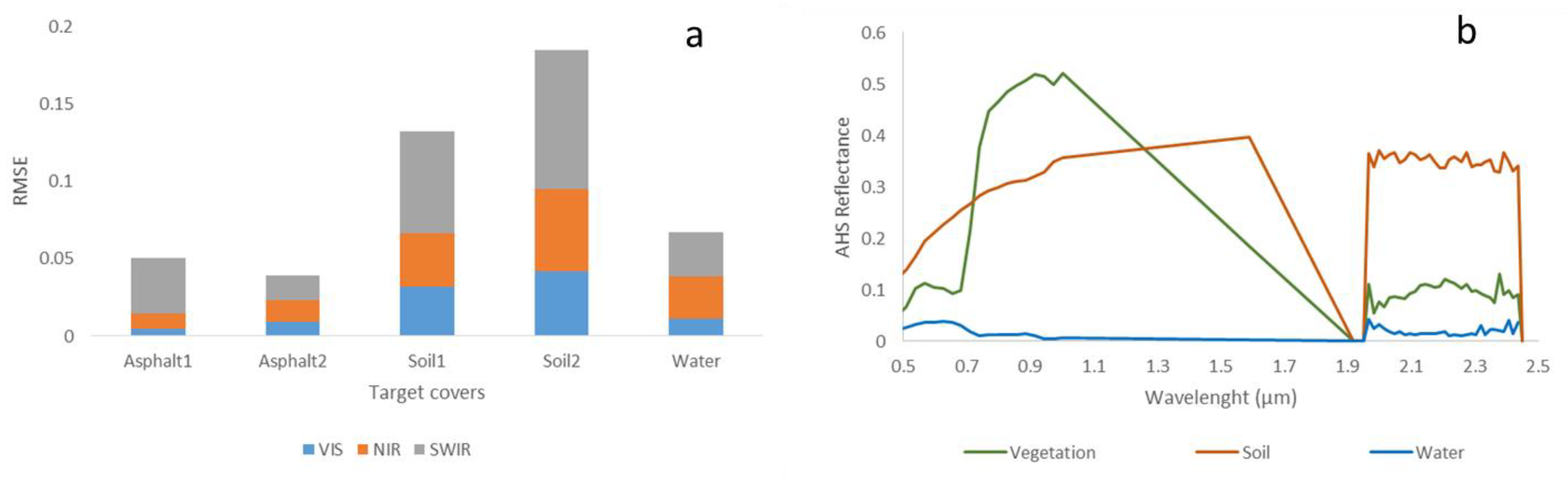
3.1. Hyperspectral Image Pre-Processing

Absolute radiometric accuracy of the image, evaluated by comparing image reflectance values with the field spectra acquired with ASD Fieldspec3 FR on invariant surfaces, showed good results. Image reflectance accurately agreed with the ASD reflectance with RMSE values ranging between 0.010 and 0.085 (Figure 3a). The absolute geographical accuracy of the images was also satisfactory with a total RMSE of 0.232 m.
Spectral profiles for selected pixels located in homogenous covers revealed anomalies in several bands acquired by the port 2 of the sensor (bands 22 to 56 from 1900 to 2600 nm). Some of these anomalies occurred when bands were located at the edge of atmospheric windows, as in bands 22 and 23 (1917 and 1933 nm, respectively), while in other bands, the problem was related with detector malfunctions, as reported by Miguel [43] (Figure 3b). In both cases, a very low signal to noise ratio (SNR) made those bands unlikely to be useful. As a result, we decided to discard all port 2 SWIR bands, therefore the final number of bands used in the classification process was 21, covering the spectral range from 456 to 1650 nm.

3.2. Image Classification: Weed Maps

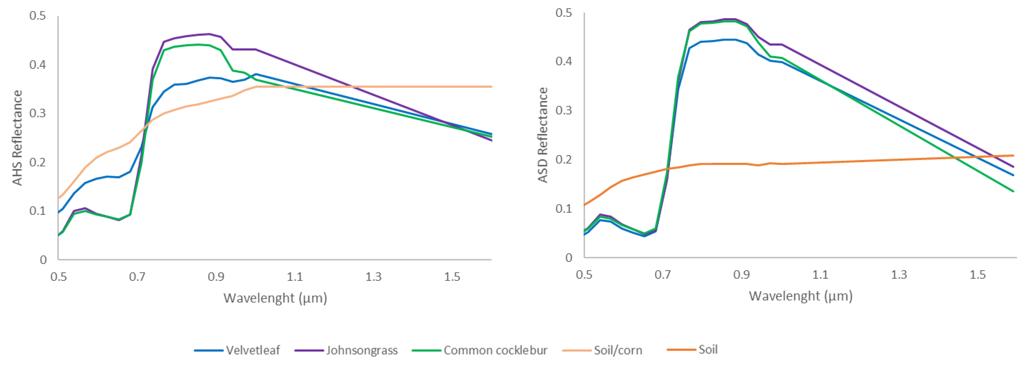
3.2.1. Endmember Selection

The PPI index applied to the AHS image enabled to identify four endmembers for johnsongrass, two for common cocklebur, two for velvetleaf and eight endmembers for soil/crop (which represents either bare soil pixels and those with a spectral mixture of soil and vegetation but with soils as the predominant cover).
Average spectra of the endmembers obtained for each target cover method from the AHS image using the PPI method (left) and field spectroscopy using a GER2600 field portable spectroradiometer (right) are shown in Figure 4. Significant differences between both methods were observed, especially for velvetleaf and soil covers. The differences were small for johnsongrass and common cocklebur but still detectable, especially in the VIS and NIR. In the VIS, these differences can be related to the soil background influence in the pixel signal that contributes to slightly increase the reflectance in the red region in the spectra obtained from the AHS image. In the NIR, the discrepancies can be related with the different observation geometry of the field and airborne sensors. For velvetleaf, the spectral signature of the endmember obtained from the image showed higher reflectance values in the VIS but lower in the NIR which could reveal the selection in the image of mixed pixels with relevant contribution from the soil background. Regarding the soil spectrum, reflectance values were consistently higher in the average endmember obtained from the image. This is likely related to the higher spectral variability of the soil cover across the image compared with the more restricted area measured with the spectroradiometer, but especially to the automatic selection of pixels with low vegetation cover (soil mixed with corn plants), which causes a typical absorption feature in the red and higher reflectance in the NIR and SWIR bands.

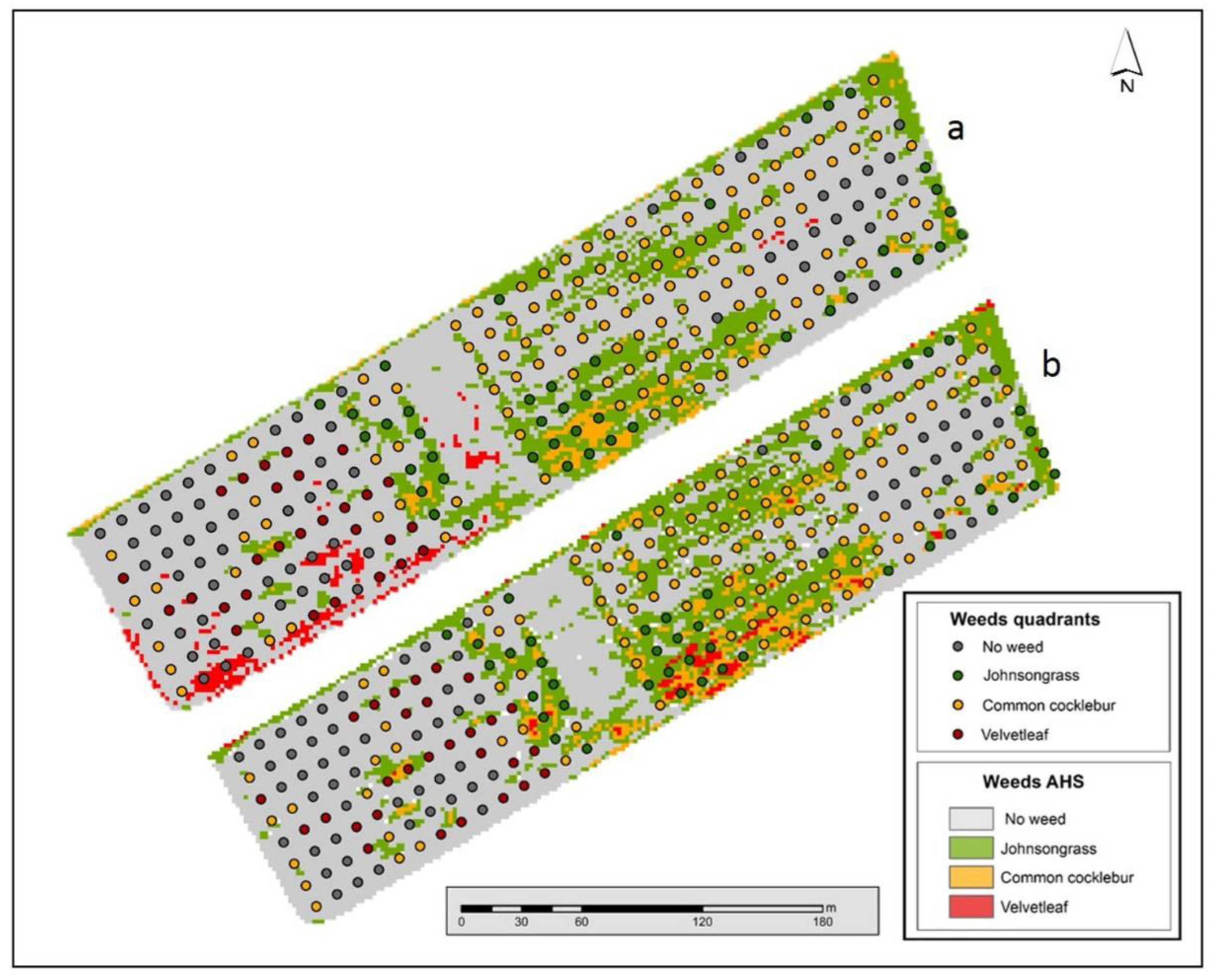
3.2.2. Spectral Angle Mapper Classification

Figure 5 shows the weed map obtained from the AHS image with the SAM classification technique using endmembers derived from field spectroscopy. This map shows no discrimination between the three weed species, but a general picture of weed infestation in the field. As it can be observed, weeds were more profusely infesting the north and northeast edges of the field and most of the central area. In contrast, the southwest half of the field was relatively clean of weeds. The higher weed abundance along the field edges is common in many agricultural farms and was previously reported for johnsongrass [25]. The uneven distribution between the two halves of the field is likely because these two sections were managed as independent fields in previous years, having different cropping histories, as noted in Section 2.1. Comparison with the field data using a challenging low biomass threshold (first quartile = 2 g m−2) which include very low density patches, showed an overall accuracy of 60.3% and a kappa coefficient of 0.20, with large omission errors, close to 75%, but low commission errors (Table 2). By increasing the biomass threshold to the median biomass value (second quartile = 12.8 g m−2), the results substantially improved, thereby decreasing the omission errors by more than 25%, while the overall accuracy and kappa coefficient increased to 0.46 (Table 2). When a very high biomass threshold was considered (third quartile = 25.4 g m−2), which means that only very dense weed patches were used for validation, the overall accuracy reached 85.1% with a kappa coefficient of 0.72 (Table 2) and 25% omission errors.
The SAM classification results using the two endmember extraction methods, PPI and field spectroscopy, for the discrimination of the three weed species are shown in Figure 6. The two maps are consistent in the classification of johnsongrass, the predominant weed species, while they differ significantly in the abundance and spatial distribution of the other two species. Classification based on PPI endmembers (Figure 6a) detects an important infestation of velvetleaf in the southwest half of the field, which is not observed in the classification obtained from field spectroscopy endmembers (Figure 6b). In this case, velvetleaf is mainly located in the center-south area of the field, mainly associated to common cocklebur patches.
The accuracy of the classification results was proven by comparison with the field data through analyzing the spatial agreement of the four classes (three weeds and soil) with the 272 sampling frames previously assigned to the predominant weed species (as described in Section 2.4). According to the confusion matrices, overall accuracies ranged from 32% to 35% (Table 3 and Table 4). Omission errors were similar regardless of whether the classification was based on PPI endmembers or field spectroscopy endmembers. In both methods, the most accurate classification resulted in johnsongrass with omission errors of 52.4% and 47.6%, respectively, whereas a low accuracy (i.e., large omission errors) was observed in common cocklebur and velvetleaf. Commission errors were also high (>42%), likely due to confusion between johnsongrass and common cocklebur, but also to confusion between vegetation and soil due to the low biomass threshold used to identify the presence of weeds in each sampling frame (first quartile = 2 g m−2).

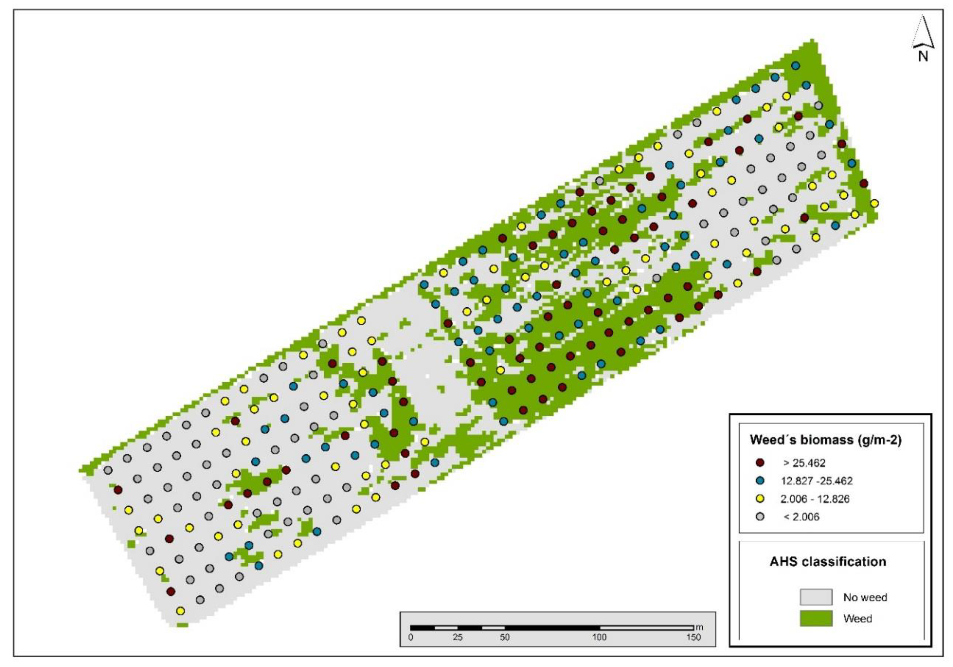
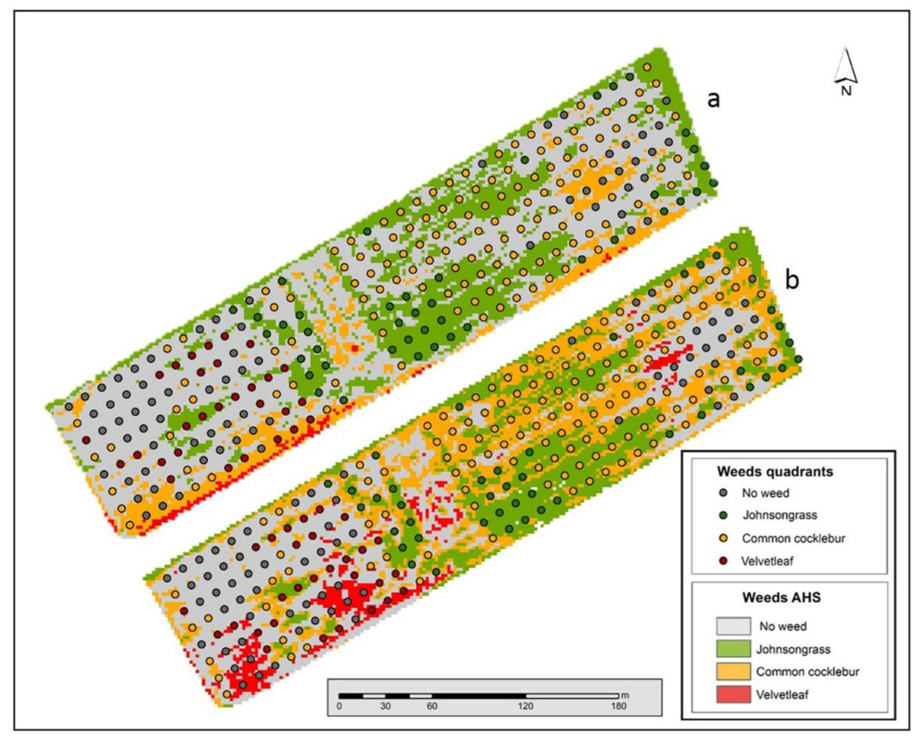
3.2.3. Spectral Mixture Analysis Classification

The weed maps obtained with the SMA classifier and the two endmember extraction techniques are shown in Figure 7. In the output images obtained with the SMA, every pixel was assigned a value representing the percentage of the area occupied by each category (weed species in this study). In order to transform these images in binary maps, a 30% threshold was selected to label a pixel as covered by weeds. This threshold was set after Martin et al. [56] who analyzed different thresholds to map johnsongrass using the SAM and concluded that 30% provided the best fit with the field data.
As in the case of the SAM, both maps were similar regarding the extent and spatial distribution of johnsongrass. However, significant differences were observed between the two maps for the other two weed species. In the map obtained using PPI endmembers (Figure 7a), velvetleaf was only detected in the southwestern edge of the field, whereas the map generated with field spectroscopy endmembers (Figure 7b) showed velvetleaf infestation over a larger area overlapping with some areas assigned to common cocklebur by using PPI.
The validation results showed the best overall accuracy and kappa values for the classification based on field spectroscopy endmembers (Table 5 and Table 6). This classification method, in general provided lower errors of commission and omission than PPI for the three weed species, although with very low accuracies for velvetleaf. The classification based in PPI endmembers showed similar results from those obtained using the SAM with a maximum overall accuracy of 32% and a kappa of 0.11. Confusion matrices revealed again high omission and commission errors for velvetleaf and common cocklebur unless the latter significantly reduced those errors in the classification obtained using field spectroscopy endmembers. Velvetleaf showed large confusions, mainly with soil/crop areas, while common cocklebur was incorrectly identified as johnsongrass except in most dense patches located in the center-south area.

4. Discussion

In recent years, advances in early season weed monitoring using remote sensing techniques have been achieved thanks to the development of UAV technology [16]. However, most of the studies so far are based on the use of RGB or multispectral cameras [57], able to obtain information in a reduced number of spectral bands, which makes it difficult to discriminate between crops and weed species when they exhibit similar spectral behavior. The use of hyperspectral sensors offers the possibility to improve the accuracy of weed detection and species discrimination. Our study demonstrated the potential of airborne hyperspectral images to generate reliable spatial information on the distribution of three major weed species in corn fields when the crop are in the optimal growing stage for the application of herbicides. Overall accuracies ranged between 60% and 80% using the SAM for maps that do not differentiate the different weed species. This agrees with results from other studies using hyperspectral airborne data to discriminate weeds in rangelands [58] where spotted knapweed was detected with the SAM classification algorithm, but only for large cover densities (>70%) and populations larger than 0.1 ha. Another study also using the SAM algorithm [59] established that 57% of known spotted knapweed infestations and 97% of known baby’s-breath infestations were identified through the use of airborne hyperspectral imagery. However, in this work, mixed pixels from associated vegetation produced high omission errors. Authors discussed the need for applying unmixing algorithms to estimate the relative fraction of each element to solve this problem as we did in our study.
The use of high spatial and spectral resolution images is intended to progress on one of the main challenges facing site-specific weed management, i.e., achieving a robust weed classification method capable of accurately detecting and mapping, not only the presence/absence of weeds, but also the different weed species [6]. The recognition of specific weed community patterns among crops allows for the design of management strategies adapted to the type and severity of the problem identified, its spatial extension and temporal evolution, and its impact on crop yield. From a crop protection point of view, early weed mapping is crucial because it coincides with the time to apply weed control measures, i.e., at the right place and at the right time. Some authors support the idea that site specific weed management does not require discrimination between weed species, but it is enough with the classification of broad leaf and grass weeds for reducing herbicide treatment [60,61]. Moreover, recent studies have demonstrated that some weed communities are not adversely affecting crop yield and quality [62]. Therefore, further research on weed population dynamics and their competition with crops are needed in order to apply this knowledge to agricultural practices so as to specifically identify and eradicate only harmful weed species [57].
Despite the improvement in species discriminability that hyperspectral information facilitates, the spectral mixture between weeds, crops and bare soil is still critical in hyperspectral weed mapping. Improved spatial resolution, as provided by images acquired from field platforms or UAVs, can contribute to solve this problem. This was proved by Scherrer et al. [23] who used both ground-based and drone-based hyperspectral imagers to discriminate for herbicide-resistant weeds. They obtained classification accuracies ranging from 77% to 99% for spectra acquired by the ground-based imaging platform and from 25% to 79% for images acquired from the drone-based platform flying 9.7 m above the crops and weeds and providing a pixel size of about 2 mm. Authors discuss the need of testing the model under multiple and varying field conditions including mixed pixels to explore the efficacy of the proposed methods. In our work we have applied a spectral unmixing methodology, the SMA, to deal with the mixed-pixel problem achieving a significant improvement (20% overall accuracy improvement) compared to the other spectral matching algorithm applied, the SAM.
A common problem to the SMA and SAM classification techniques is the definition of the pure/reference spectra. The two different endmember extraction techniques compared in our study, in-situ spectral measurements of “pure” covers and automatic identification of “pure” pixels in the image, indicates that field spectroscopy can provide complementary information useful for weed mapping using airborne hyperspectral imagery, where pixel sizes > 1 m are common, but which is also applicable to those obtained from UAV platforms with smaller pixels. We propose a new field protocol that allows for obtaining pure endmember spectra of the different weed species by reproducing homogeneous canopies and avoiding soil background effects. However, the inherent image noise, primarily related to the acquisition conditions (atmospheric and illumination effects) can cause discrepancies between the measured response in the field and captured by the sensor, causing poor endmember characterization using field spectroscopy. The use of the EL method to improve image radiometric calibration by forcing image data to match selected field reflectance spectra obtained over invariant surfaces, has contributed to reduce those discrepancies. Using image-based extraction methods, such as the PPI, bypasses the need for ground spectral measurements as well as the need to obtain accurate image radiometric calibrations. However, to identify pure pixels in crop fields, it is often extremely difficult given the heterogeneity of the target covers at the remote sensing scale, even at a very high spatial resolution, as is the case in using airborne sensors. In our study, the endmember selection based on field spectroscopy outperformed the image-based extraction method, especially in the SMA classification were the former improved by 20% in the overall classification accuracy.
Johnsongrass, always offered the lower omission errors both with the SMA (40.5% to 52.4%) and SAM (33.3 % to 47.6%), probably because it was concentrated in more dense patches. The SMA offered better results than the SAM when compared with the field data for the other two weed species (common cocklebur and velvetleaf) but both classification methods failed to identify velvetleaf (omission errors >96%), which can be related to the smaller validation sample and the lower biomass of this species in the study site.
The weed map obtained with the SMA and field spectroscopy endmembers is quite precisely reflecting the history of the field and its influence on weed infestations (Figure 7b). The eastern part of the field, which had been planted with corn in the preceding 5 years, shows higher infestation and different species (mainly common cocklebur and johnsongrass) than the western part, where the previous corn crop was followed by three years of barley cropping. It is also interesting to see how the area between these two subplots shows also a clear distinctive pattern, with little and very variable infestation. This location overlapped with the area where a small fertilization experiment was conducted several years prior to the hyperspectral flight (C. Fernández-Quintanilla, personal communication).
Even though the high cost of acquiring airborne hyperspectral images limits the operational use of the proposed methodology, our work demonstrates its potential application to low cost images provided by new hyperspectral sensors onboard UAVs. The emergence of a new generation of UAVs with advanced cameras and sensors either by combining optical, thermal and Lidar instruments, or by increasing the spectral resolution of the optical cameras by up to tens/hundreds of bands in the VIS-NIR, but also in the SWIR regions, will facilitate the accurate monitoring of weeds causing damage by competition with crops. The methods proposed in our study can be also applicable to recognize specific patterns typical of weed invasive species, such as Amaranthus palmeri in corn [63] and Centaurea maculosa and Gypsophila paniculata in semiarid rangeland and irrigated pastures [59]. Based on spectral characteristics of invasive plants, these may be detectable at late growing stages when the plant community [64] or the structure of the agricultural habitat [65] is changing, using the new generation of hyperspectral satellite sensors, such as the Italian Hyperspectral Precursor of the Application Mission (PRISMA) or the German Environmental Mapping and Analysis Program (EnMAP).

Author Contributions

Conceptualization, M.P.M., C.F.-Q. and J.D.; investigation and methodology, M.P.M., B.P., C.F.-Q. and J.D.; validation, M.P.M., C.F.-Q., P.E. and J.D.; software and formal analysis, M.P.M., B.P. and P.E.; writing—original draft preparation, M.P.M.; writing—review and editing, M.P.M., C.F.-Q. and J.D.; funding acquisition, C.F.-Q. and J.D. All authors have read and agreed to the published version of the manuscript.

Funding

This research was supported by the Spanish Research State Agency (AEI) through the Project PID2020-113229RB-C41/AEI/10.13039/501100011033.

Data Availability Statement

The data that support the findings of this study are available from the corresponding author, [M.P.M.], upon reasonable request.

Acknowledgments

We would like to thank all people involved during the field campaigns from different institutions: SpecLab-CSIC, ICA-CSIC, University of Alcalá and INTA, as well as to the technical staff of the CSIC experimental farm “La Poveda” for their support in the implementation of the field experimentation.

Conflicts of Interest

The authors declare no conflict of interest.

References

  1. Christensen, S.; Søgaard, H.T.; Kudsk, P.; Nørremark, M.; Lund, I.; Nadimi, E.S.; Jørgensen, R. Site-specific weed control technologies. Weed Res. 2009, 49, 233–241. [Google Scholar] [CrossRef]
  2. Fernández-Quintanilla, C.; Dorado, J.; Andújar, D.; Peña, J.M. Site-Specific Based Models. In Decision Support Systems for Weed Management; Chantre, G.R., González-Andújar, J.L., Eds.; Springer International Publishing: Cham, Switzerland, 2020; pp. 143–157. [Google Scholar]
  3. Fernandez-Quintanilla, C.; Dorado, J.; Andújar, D.; Peña-Barragán, J.M. Advanced detection technologies for weed scouting. In Advances in Integrated Weed Management; Kudsk, P., Ed.; Burleigh Dodds Science Publishing: Cambridge, UK, 2022; pp. 205–227. [Google Scholar]
  4. Fernández-Quintanilla, C.; Peña, J.M.; Andújar, D.; Dorado, J.; Ribeiro, A.; López-Granados, F. Is the current state of the art of weed monitoring suitable for site-specific weed management in arable crops? Weed Res. 2018, 58, 259–272. [Google Scholar] [CrossRef]
  5. Gerhards, R.; Andújar, D.; Hamouz, P.; Peteinatos, G.G.; Christensen, S.; Fernandez-Quintanilla, C. Advances in site-specific weed management in agriculture—A review. Weed Res. 2022, 62, 123–133. [Google Scholar] [CrossRef]
  6. Lati, R.N.; Rasmussen, J.; Andujar, D.; Dorado, J.; Berge, T.W.; Wellhausen, C.; Pflanz, M.; Nordmeyer, H.; Schirrmann, M.; Eizenberg, H.; et al. Site-specific weed management—Constraints and opportunities for the weed research community: Insights from a workshop. Weed Res. 2021, 61, 147–153. [Google Scholar] [CrossRef]
  7. López-Granados, F. Weed detection for site-specific weed management: Mapping and real-time approaches. Weed Res. 2011, 51, 1–11. [Google Scholar] [CrossRef]
  8. Andújar, D.; Calle, M.; Fernández-Quintanilla, C.; Ribeiro, A.; Dorado, J. Three-Dimensional Modeling of Weed Plants Using Low-Cost Photogrammetry. Sensors 2018, 18, 1077. [Google Scholar] [CrossRef]
  9. Longchamps, L.; Panneton, B.; Simard, M.-J.; Leroux, G.D. A Technique for High-Accuracy Ground-Based Continuous Weed Mapping at Field Scale. Trans. ASABE 2013, 56, 1523–1533. [Google Scholar] [CrossRef]
  10. Weis, M.; Sökefeld, M. Detection and Identification of Weeds. In Precision Crop Protection—The Challenge and Use of Heterogeneity; Oerke, E.-C., Gerhards, R., Menz, G., Sikora, R.A., Eds.; Springer: Dordrecht, The Netherlands, 2010; pp. 119–134. [Google Scholar]
  11. Martín, M.P.; Barreto, L.; Fernández-Quintanilla, C. Discrimination of sterile oat (Avena sterilis) in winter barley (Hordeum vulgare) using QuickBird satellite images. Crop Prot. 2011, 30, 1363–1369. [Google Scholar] [CrossRef]
  12. Zhang, Y.; Slaughter, D.C.; Staab, E.S. Robust hyperspectral vision-based classification for multi-season weed mapping. ISPRS J. Photogramm. Remote Sens. 2012, 69, 65–73. [Google Scholar] [CrossRef]
  13. Lamb, D.W.; Brown, R.B. PA—Precision Agriculture: Remote-Sensing and Mapping of Weeds in Crops. J. Agric. Eng. Res. 2001, 78, 117–125. [Google Scholar] [CrossRef]
  14. Lamb, D.W.; Weedon, M. Evaluating the accuracy of mapping weeds in fallow fields using airborne digital imaging: Pancium effusum in oilseed rape stubble. Weed Res. 1998, 38, 443–451. [Google Scholar] [CrossRef]
  15. Peña-Barragán, J.M.; Torres-Sánchez, J.; de Castro, A.; Kelly, M.; López-Granados, F. Weed Mapping in Early-Season Maize Fields Using Object-Based Analysis of Unmanned Aerial Vehicle (UAV) Images. PLoS ONE 2013, 8, e77151. [Google Scholar] [CrossRef]
  16. de Castro, A.I.; Torres-Sánchez, J.; Peña, J.M.; Jiménez-Brenes, F.M.; Csillik, O.; López-Granados, F. An Automatic Random Forest-OBIA Algorithm for Early Weed Mapping between and within Crop Rows Using UAV Imagery. Remote Sens. 2018, 10, 285. [Google Scholar] [CrossRef]
  17. Che’Ya, N.N.; Ernest, D.; Madan, G. Assessment of Weed Classification Using Hyperspectral Reflectance and Optimal Multispectral UAV Imagery. Agronomy 2021, 11, 1435. [Google Scholar] [CrossRef]
  18. de Castro, A.I.; Jurado-Expósito, M.; Gómez-Casero, M.-T.; López-Granados, F. Applying Neural Networks to Hyperspectral and Multispectral Field Data for Discrimination of Cruciferous Weeds in Winter Crops. Sci. World J. 2012, 2012, 630390. [Google Scholar] [CrossRef] [PubMed]
  19. Martín, M.P.; Barreto, L.; Riaño, D.; Fernandez-Quintanilla, C.; Vaughan, P. Assessing the potential of hyperspectral remote sensing for the discrimination of grassweeds in winter cereal crops. Int. J. Remote Sens. 2011, 32, 49–67. [Google Scholar] [CrossRef]
  20. Gao, J.; Nuyttens, D.; Lootens, P.; He, Y.; Pieters, J.G. Recognising weeds in a maize crop using a random forest machine-learning algorithm and near-infrared snapshot mosaic hyperspectral imagery. Biosyst. Eng. 2018, 170, 39–50. [Google Scholar] [CrossRef]
  21. Li, Y.; Al-Sarayreh, M.; Irie, K.; Hackell, D.; Bourdot, G.; Reis, M.M.; Ghamkhar, K. Identification of Weeds Based on Hyperspectral Imaging and Machine Learning. Front. Plant Sci. 2021, 11, 611622. [Google Scholar] [CrossRef]
  22. Okamoto, H.; Murata, T.; Kataoka, T.; Hata, S.-I. Plant classification for weed detection using hyperspectral imaging with wavelet analysis. Weed Biol. Manag. 2007, 7, 31–37. [Google Scholar] [CrossRef]
  23. Scherrer, B.; Sheppard, J.; Jha, P.; Shaw, J.A. Hyperspectral imaging and neural networks to classify herbicide-resistant weeds. J. Appl. Remote Sens. 2019, 13, 044516. [Google Scholar] [CrossRef]
  24. Andújar, D.; Barroso, J.; Fernández-Quintanilla, C.; Dorado, J. Spatial and temporal dynamics of Sorghum halepense patches in maize crops. Weed Res. 2012, 52, 411–420. [Google Scholar] [CrossRef]
  25. Andújar, D.; Ruiz, D.; Ribeiro, A.; Fernández-Quintanilla, C.; Dorado, J. Spatial Distribution Patterns of Johnsongrass (Sorghum halepense) in Corn Fields in Spain. Weed Sci. 2011, 59, 82–89. [Google Scholar] [CrossRef]
  26. Gray, C.J.; Shaw, D.R.; Gerard, P.D.; Bruce, L.M. Utility of Multispectral Imagery for Soybean and Weed Species Differentiation. Weed Technol. 2008, 22, 713–718. [Google Scholar] [CrossRef]
  27. Medlin, C.R.; Shaw, D.R.; Gerard, P.D.; LaMastus, F.E. Using remote sensing to detect weed infestations in Glycine max. Weed Sci. 2000, 48, 393–398. [Google Scholar] [CrossRef]
  28. AVIRIS. Available online: https://aviris.jpl.nasa.gov (accessed on 3 January 2023).
  29. APEX. Available online: https://apex-esa.org (accessed on 10 January 2023).
  30. Goel, P.K.; Prasher, S.O.; Landry, J.A.; Patel, R.M.; Bonnell, R.B.; Viau, A.A.; Miller, J.R. Potential of airborne hyperspectral remote sensing to detect nitrogen deficiency and weed infestation in corn. Comput. Electron. Agric. 2003, 38, 99–124. [Google Scholar] [CrossRef]
  31. Karimi, Y.; Prasher, S.O.; McNairn, H.; B. Bonnell, R.; Dutilleul, P.; K. Goel, P. Classification accuracy of discriminant analysis, artificial neural networks, and decision trees for weed and nitrogen stress detection in corn. Trans. ASAE 2005, 48, 1261–1268. [Google Scholar] [CrossRef]
  32. Yang, C.; Everitt, J.H. Mapping three invasive weeds using airborne hyperspectral imagery. Ecol. Inform. 2010, 5, 429–439. [Google Scholar] [CrossRef]
  33. Singh, V.; Rana, A.; Bishop, M.; Filippi, A.M.; Cope, D.; Rajan, N.; Bagavathiannan, M. Chapter Three—Unmanned aircraft systems for precision weed detection and management: Prospects and challenges. In Advances in Agronomy; Sparks, D.L., Ed.; Academic Press: Cambridge, MA, USA, 2020; Volume 159, pp. 93–134. [Google Scholar]
  34. Gogineni, R.; Chaturvedi, A. Hyperspectral Image Classification. In Processing and Analysis of Hyperspectral Data; Jie, C., Yingying, S., Hengchao, L., Eds.; IntechOpen: Rijeka, Croatia, 2019; Chapter 2. [Google Scholar]
  35. Vyas, D.; Krishnayya, N.S.R.; Manjunath, K.R.; Ray, S.S.; Panigrahy, S. Evaluation of classifiers for processing Hyperion (EO-1) data of tropical vegetation. Int. J. Appl. Earth Obs. Geoinf. 2011, 13, 228–235. [Google Scholar] [CrossRef]
  36. Kumar, M.N.; Seshasai, M.V.R.; Vara Prasad, K.S.; Kamala, V.; Ramana, K.V.; Dwivedi, R.S.; Roy, P.S. A new hybrid spectral similarity measure for discrimination among Vigna species. Int. J. Remote Sens. 2011, 32, 4041–4053. [Google Scholar] [CrossRef]
  37. South, S.; Qi, J.; Lusch, D.P. Optimal classification methods for mapping agricultural tillage practices. Remote Sens. Environ. 2004, 91, 90–97. [Google Scholar] [CrossRef]
  38. Plaza, A.; Benediktsson, J.A.; Boardman, J.W.; Brazile, J.; Bruzzone, L.; Camps-Valls, G.; Chanussot, J.; Fauvel, M.; Gamba, P.; Gualtieri, A.; et al. Recent advances in techniques for hyperspectral image processing. Remote Sens. Environ. 2009, 113, S110–S122. [Google Scholar] [CrossRef]
  39. Miao, X.; Gong, P.; Swope, S.; Pu, R.; Carruthers, R.; Anderson, G.L.; Heaton, J.S.; Tracy, C.R. Estimation of yellow starthistle abundance through CASI-2 hyperspectral imagery using linear spectral mixture models. Remote Sens. Environ. 2006, 101, 329–341. [Google Scholar] [CrossRef]
  40. San Martín, C.; Andújar, D.; Fernández-Quintanilla, C.; Dorado, J. Spatial Distribution Patterns of Weed Communities in Corn Fields of Central Spain. Weed Sci. 2015, 63, 936–945. [Google Scholar] [CrossRef]
  41. Jhala, A.J.; Knezevic, S.Z.; Ganie, Z.A.; Singh, M. Integrated weed management in maize. In Recent Advances in Weed Management; Springer: New York, NY, USA, 2014; pp. 177–196. [Google Scholar]
  42. Dieleman, J.A.; Mortensen, D.A. Characterizing the spatial pattern of Abutilon theophrasti seedling patches. Weed Res. 1999, 39, 455–467. [Google Scholar] [CrossRef]
  43. Miguel, E.d.; Jimenez, M.; Pérez, I.; Cámara, O.G.d.l.; Muñoz, F.; Gomez-Sanchez, J.A. AHS and CASI Processing for the REFLEX Remote Sensing Campaign: Methods and Results. Acta Geophys. 2015, 63, 1485–1498. [Google Scholar] [CrossRef]
  44. Van Cleemput, E.; Roberts, D.A.; Honnay, O.; Somers, B. A novel procedure for measuring functional traits of herbaceous species through field spectroscopy. Methods Ecol. Evol. 2019, 10, 1332–1338. [Google Scholar] [CrossRef]
  45. Ben-Dor, E.; Kindel, B.; Goetz, A.F.H. Quality assessment of several methods to recover surface reflectance using synthetic imaging spectroscopy data. Remote Sens. Environ. 2004, 90, 389–404. [Google Scholar] [CrossRef]
  46. Chi, M.; Feng, R.; Bruzzone, L. Classification of hyperspectral remote-sensing data with primal SVM for small-sized training dataset problem. Adv. Space Res. 2008, 41, 1793–1799. [Google Scholar] [CrossRef]
  47. Alajlan, N.; Bazi, Y.; Melgani, F.; Yager, R.R. Fusion of supervised and unsupervised learning for improved classification of hyperspectral images. Inf. Sci. 2012, 217, 39–55. [Google Scholar] [CrossRef]
  48. Debba, P.; van Ruitenbeek, F.J.A.; van der Meer, F.D.; Carranza, E.J.M.; Stein, A. Optimal field sampling for targeting minerals using hyperspectral data. Remote Sens. Environ. 2005, 99, 373–386. [Google Scholar] [CrossRef]
  49. Roberts, D.A.; Numata, I.; Holmes, K.; Batista, G.; Krug, T.; Monteiro, A.; Powell, B.; Chadwick, O.A. Large area mapping of land-cover change in Rondônia using multitemporal spectral mixture analysis and decision tree classifiers. J. Geophys. Res. Atmos. 2002, 107, LBA 40-41-LBA 40-18. [Google Scholar] [CrossRef]
  50. Jiménez-Muñoz, J.C.; Sobrino, J.A.; Plaza, A.; Guanter, L.; Moreno, J.; Martínez, P. Comparison Between Fractional Vegetation Cover Retrievals from Vegetation Indices and Spectral Mixture Analysis: Case Study of PROBA/CHRIS Data Over an Agricultural Area. Sensors 2009, 9, 768–793. [Google Scholar] [CrossRef] [PubMed]
  51. Kruse, F.A.; Lefkoff, A.B.; Boardman, J.W.; Heidebrecht, K.B.; Shapiro, A.T.; Barloon, P.J.; Goetz, A.F.H. The spectral image processing system (SIPS)—Interactive visualization and analysis of imaging spectrometer data. Remote Sens. Environ. 1993, 44, 145–163. [Google Scholar] [CrossRef]
  52. Shimabukuro, Y.E.; Ponzoni, F.J. The Linear Spectral Mixture Model. In Spectral Mixture for Remote Sensing: Linear Model and Applications; Springer International Publishing: Cham, Switzerland, 2019; pp. 23–41. [Google Scholar]
  53. Chein, I.C.; Plaza, A. A fast iterative algorithm for implementation of pixel purity index. IEEE Geosci. Remote Sens. Lett. 2006, 3, 63–67. [Google Scholar] [CrossRef]
  54. Andújar, D.; Ribeiro, A.; Carmona, R.; Fernández-Quintanilla, C.; Dorado, J. An assessment of the accuracy and consistency of human perception of weed cover. Weed Res. 2010, 50, 638–647. [Google Scholar] [CrossRef]
  55. Hudson, W.D.; Ramm, C.W. Correct formulation of the Kappa coefficient of agreement. Photogramm. Eng. Remote Sens. 1987, 53, 421–422. [Google Scholar]
  56. Martín, M.P.; Barreto, L.; Riaño, D.; Fernández-Quintanilla, C.; Vaughan, P.; De Santis, A. Cartografía de malas hierbas en cultivos de maíz mediante imágenes hiperespectrales aeroportadas (AHS). In Proceedings of the XIII Congreso de la Asociación Española de Teledetección Agua y Desarrollo Sostenible, Calatayud, Spain, 23–26 September 2009; pp. 41–44. [Google Scholar]
  57. Esposito, M.; Crimaldi, M.; Cirillo, V.; Sarghini, F.; Maggio, A. Drone and sensor technology for sustainable weed management: A review. Chem. Biol. Technol. Agric. 2021, 8, 18. [Google Scholar] [CrossRef]
  58. Lass, L.W.; Thill, D.C.; Shafii, B.; Timothy, S.P. Detecting Spotted Knapweed (Centaurea maculosa) with Hyperspectral Remote Sensing Technology. Weed Technol. 2002, 16, 426–432. [Google Scholar] [CrossRef]
  59. Lass, L.W.; Prather, T.S.; Glenn, N.F.; Weber, K.T.; Mundt, J.T.; Pettingill, J. A Review of Remote Sensing of Invasive Weeds and Example of the Early Detection of Spotted Knapweed (Centaurea maculosa) and Babysbreath (Gypsophila paniculata) with a Hyperspectral Sensor. Weed Sci. 2005, 53, 242–251. [Google Scholar] [CrossRef]
  60. Gibson, K.D.; Richard, D.; Case, R.M.; Loree, J. Detection of Weed Species in Soybean Using Multispectral Digital Images. Weed Technol. 2004, 18, 742–749. [Google Scholar] [CrossRef]
  61. Thorp, K.R.; Tian, L.F. A Review on Remote Sensing of Weeds in Agriculture. Precis. Agric. 2004, 5, 477–508. [Google Scholar] [CrossRef]
  62. Gibson, D.J.; Young, B.G.; Wood, A.J. Can weeds enhance profitability? Integrating ecological concepts to address crop-weed competition and yield quality. J. Ecol. 2017, 105, 900–904. [Google Scholar] [CrossRef]
  63. Torra, J.; Royo-Esnal, A.; Romano, Y.; Osuna, M.D.; León, R.G.; Recasens, J. Amaranthus palmeri a New Invasive Weed in Spain with Herbicide Resistant Biotypes. Agronomy 2020, 10, 993. [Google Scholar] [CrossRef]
  64. Karnieli, A.; Bayarjargal, Y.; Bayasgalan, M.; Mandakh, B.; Dugarjav, C.; Burgheimer, J.; Khudulmur, S.; Bazha, S.N.; Gunin, P.D. Do vegetation indices provide a reliable indication of vegetation degradation? A case study in the Mongolian pastures. Int. J. Remote Sens. 2013, 34, 6243–6262. [Google Scholar] [CrossRef]
  65. Matongera, T.N.; Mutanga, O.; Dube, T.; Lottering, R.T. Detection and mapping of bracken fern weeds using multispectral remotely sensed data: A review of progress and challenges. Geocarto Int. 2018, 33, 209–224. [Google Scholar] [CrossRef]
Figure 1. Experimental configuration of field spectral measurements of pure weed covers. The lower part of the tray shows the inserted stems that allow for replicating plant structure (a). The upper part of the tray is covered with black paper to avoid background contribution to the measured weed´s pure signal (b).
Agronomy 13 00528 g001
Figure 2. Workflow diagram of the AHS image classification process.
Agronomy 13 00528 g002
Figure 3. RMSE average values between the AHS image and ASD field spectroscopy reflectance obtained for each spectral region (VIS, NIR and SWIR) over selected homogeneous reference targets (asphalt, soil and water) (a); and spectral signatures of vegetation, soil and water covers using all original AHS bands where anomalous SWIR port 2 channels (1917 to 2449 nm) can be identified (b).
Agronomy 13 00528 g003
Figure 4. Spectral signature of the endmembers obtained from the AHS image using the PPI method (left) and from pure weed covers and field spectroscopy (right).
Agronomy 13 00528 g004
Figure 5. Weed map including all weed species in the field, as obtained from the AHS image classification using the SAM and field spectroscopy endmembers. Colored circles show, as a visual reference, the location of the 272 sampling frames used for validation purposes and the total biomass of all weed species identified in each frame.
Agronomy 13 00528 g005
Figure 6. Weed maps obtained from the AHS image classification using the SAM + PPI endmembers (a) and the SAM + field spectroscopy endmembers (b). Colored circles show, as a visual reference, the location of the 272 frames sampled in the field. Each sampling frame has been assigned to the most abundant weed species.
Agronomy 13 00528 g006
Figure 7. Weed maps obtained from the AHS image classification using the SMA + PPI endmembers (a) or the SMA + field spectroscopy endmembers (b). Colored circles show, as a visual reference, the location of the 272 frames sampled in the field. Each sampling frame has been assigned to the most abundant weed species.
Agronomy 13 00528 g007
Table 1. AHS spectral configuration.
Port 1
VIS/NIR
Port 2A
SWIR
Port 2
SWIR
Port 3
MIR
Port 4
TIR
Spectral range (nm)440–1020 1490–16501900–26003000–55008000–13,000
Bandwidth (nm)281601830–40400–550
Number of bands20142710
Table 2. Results of the weed classification obtained with the AHS image using the SAM and field spectroscopy endmembers.
Weed Biomass Threshold/
Quartiles *
(g m−2)
CoverCommission ErrorOmission
Error
Overall
Accuracy
Kappa
Coefficient
Q1 = 2.006Weeds15.875.460.30.20
Soil/crop43.74.5
Q2 = 12.826Weeds7.949.272.60.46
Soil/crop354.5
Q3 = 25.462Weeds5.52585.10.72
Soil/crop21.24.5
* Q1 is the first quartile (25% of the data are below this value); Q2 is the second quartile or median and Q3 is the third quartile (25% of the data are above this value).
Table 3. Confusion matrix for the AHS image classification using the SAM and PPI endmembers.
Ground Truth
AHS Soil/CropJohnsongrassCommon
Cocklebur
VelvetleafTotalCommission
Error (%)
Soil/Crop6617912720167.2
Johnsongrass0204116267.7
Common Cocklebur05005100
Velvetleaf 2011475
Total684213329272
Omission
Error (%)
2.952.410096.5
Overall accuracy = 32%, kappa = 0.12.
Table 4. Confusion matrix for the AHS image classification using the SAM and field spectroscopy endmembers.
Ground Truth
AHS Soil/CropJohnsongrassCommon
Cocklebur
VelvetleafTotalCommission
Error (%)
Soil/Crop651672416761
Johnsongrass3225648574.1
Common Cocklebur05811442.8
Velvetleaf 04004100
Total684213129270
Omission Error (%)4.447.693.9100
Overall accuracy = 35%, kappa = 0.16.
Table 5. Confusion matrix for the AHS image classification using the SMA and PPI endmembers.
Ground Truth
AHS Soil/CropJohnsongrassCommon
Cocklebur
VelvetleafTotalCommission
Error (%)
Soil/Crop5816811917466.6
Johnsongrass2254778169.1
Common
Cocklebur
8153177.6
Velvetleaf 00000-
Total684213329272
Omission
Error (%)
17.740.596.2100
Overall accuracy = 32%, kappa = 0.11.
Table 6. Confusion matrix for the AHS image classification using the SMA and field spectroscopy endmembers.
Ground Truth
AHS Soil/CropJohnsongrassCommon CockleburVelvetleafTotalCommission Error (%)
Soil/Crop534311610449
Johnsongrass0284327361.6
Common Cocklebur101059108933.7
Velvetleaf 5001683.3
Total684213329272
Omission Error (%)2233.355.696.5
Overall accuracy = 52%, kappa = 0.31.
Disclaimer/Publisher’s Note: The statements, opinions and data contained in all publications are solely those of the individual author(s) and contributor(s) and not of MDPI and/or the editor(s). MDPI and/or the editor(s) disclaim responsibility for any injury to people or property resulting from any ideas, methods, instructions or products referred to in the content.

