Article

Nitrate Content Assessment in Spinach: Exploring the Potential of Spectral Reflectance in Open Field Experiments

by
Fabio Stagnari
1,
Walter Polilli
1,2,
Gabriele Campanelli
2,
Cristiano Platani
2,
Flaviano Trasmundi
1,
Gianpiero Scortichini
3 and
Angelica Galieni
2,*
1
Faculty of Bioscience and Technologies for Food, Agriculture and Environment, University of Teramo, Via Carlo Lerici 1, 64023 Teramo, Italy
2
Council for Agricultural Research and Economics, Research Centre for Vegetable and Ornamental Crops, Via Salaria 1, 63030 Monsampolo del Tronto, Italy
3
Istituto Zooprofilattico Sperimentale dell’Abruzzo e del Molise G. Caporale, Via Campo Boario, 64100 Teramo, Italy
*
Author to whom correspondence should be addressed.
Agronomy 2023, 13(1), 193; https://doi.org/10.3390/agronomy13010193
Submission received: 19 December 2022 / Revised: 3 January 2023 / Accepted: 5 January 2023 / Published: 7 January 2023
(This article belongs to the Special Issue Advances in Field Spectroscopy in Agriculture)

Abstract

:
A rapid, non-destructive method for nitrate content assessment is essential for a rational wide-scale application of nitrogen in sustainable growing spinach. The method should be effective in facing environmental, genotype, and management variability. The results from three field experiments carried out in Teramo (Italy), during the 2021 and 2022 growing seasons, and by combining nitrogen supply with spinach genotypes, are presented. The spectral canopy reflectance was collected to find out the spectral band relationship with nitrate concentration. Preliminary PCA and mixed linear model analysis showed that nitrate content is among the less detectable features. Unexpected chlorosis onset in one experiment added more variability; nevertheless, spectral regions of blue-cyan and early NIR when combined into Vegetation Indexes were able to correlate to nitrate content with R2 up to 0.65 in all experiments. This study demonstrates that focusing on just a few spectral regions facilitates the acquisition of suitable and robust information on nitrate content in spinach.

1. Introduction

Nitrates are naturally occurring polyatomic ions in soil and water and are essential for plant growth. Their accumulation into plant tissues differs among crops [1] and plant organs [2], and it can be modulated through agricultural management [3] and, with the willingness to accept trade-offs in terms of product quality loss, post-harvest techniques [4].
Among food vegetables, spinach is often found to be in the midst of the richest in nitrates [5], which makes it one of the most important sources of human nitrate dietary intake; controlling spinach nitrate content leads to modulating and assessing a large part of nitrate in the human diet.
Dietary nitrate gained attention in the 1970s, when it was recognized as responsible for methaemoglobinaemia in infants [6]. Nowadays, the health-related effect of dietary nitrates is highly debated. While the field of application of nitrates-related cancer-risk-increase shrinks—e.g., cases where there is a lack of specific polyphenols intake or the use of foods where there is a prior conversion into N-nitroso compounds [7]—the amount of convincing evidence supporting the pivotal role of dietary nitrate as a health-promoting factor with cardiovascular beneficial effects on blood pressure, as well as endothelial function, cognitive function, and exercise performance, is growing [8,9].
Although the ambivalent role of nitrates in human health is not controversial in the academy, from the legislative point of view, farmers have yet to cope with local regulations about nitrate content in crops, as it determines the industrial use after harvesting (i.e., baby food production, preserved, frozen or fresh) [10].
Applying rational fertilization management and sustainable agricultural practices, to avoid excessive nitrate accumulation, is very difficult when the approach is empirical. Consequently, farmers may rely on assessment tools that can provide an accurate estimation of nitrate content in plants. Some examples of such devices are nitrate-selective electrodes and nitrate-sensitive test strips [11] that directly measure the sap nitrate concentration. However, these devices are not widely applied due to the inconvenient number of procedures required (i.e., sampling, preservation, extraction, dilution) [12]. Other approaches are prone to carrying out the endeavor using Soil Plant Analysis Development (SPAD) and Normalized Difference Vegetation Index (NDVI) values. Such methods are non-destructive, can be used in both proximal and remote sensing, and rely on the relationship between chlorophyll, nitrogen, and nitrate to provide an indirect estimation of nitrate content. That relationship is subject to change with phenological phases, plant genotype, and agricultural practices [13,14,15].
Unlike the previously described, reflectance spectroscopy is a powerful tool, as it can measure the amount of light that, after the interaction with the plant tissue, is reflected off, bringing detailed information about the spectral profile as well as crop status [16]. It has been successfully used for screening and assessment of nitrate content in plant organs, although to our knowledge, only a few studies focused on spinach. They relied principally on the solid statistical modelling of NIR spectra [17,18,19] as well as on laboratory simulation for the spectral acquisitions [20,21,22]; the result was that the nitrate content was excellently estimated, but further steps toward easy and convenient application in field growing conditions are still to be addressed.
It is worth pinpointing that this technology requires specialized equipment, is expensive and complex to operate, and may be not available to farmers. Additionally, it requires a high level of technical expertise and knowledge to interpret data related to different types of soil or climate conditions [23,24].
On the basis of the aforementioned considerations, the scope of this study was to find an accessible pathway to transfer the sensing technology to assess nitrate content in spinach in a scalable manner. Firstly, the full power of reflectance spectroscopy was applied within open field environments (three-year field experiments) assessing its robustness against genotype, climatic conditions, and agronomical management variability. Secondly, spectral acquisitions were performed using the sensor under passive mode (i.e., solar radiation as the light source) to obtain field-scaled results coping with plant canopy architecture and environmental issues. Lastly, the complexity of the collected data was reduced: techniques such as dimensional reduction, waveband relevance exploration, and scouting for Vegetation Indexes (VIs) were applied. This approach led to novel knowledge that incorporates both robustness and convenience, as the understructure for facilitating future technology transfer.

2. Materials and Methods

2.1. Field Experiments

Three field experiments were carried out within an area typical for spinach cultivation (Table 1), located in the Sant’Omero municipality (TE), Italy. The farm “Pancottini Dante” was involved due to its experience in managing mainly horticultural crops (i.e., spinach for the deep-freezing chain). Spinach (Spinacia oleracea L.) was grown in all three experimental fields (named Exp. A, B, and C, respectively; Table 1); French bean represented the previous crop. The physical and chemical soil characteristics were: 30% sand, 45% silt, and 25% clay, pH 8.0, 1.1% organic matter, 19.0% total CaCO3, 10.6% active CaCO3, and 32.1 meq 100 g−1 cation-exchange capacity, total N 0.9 g kg−1. Physical-chemical parameters were determined following the official methods of soil analyses [25].
The area of each experiment was obtained by delimiting a surface of 30 × 60 m within the spinach-growing fields. All the crop management practices, except for fertilization treatments, followed the agronomic practices normally adopted by farmers. Within the delimited area, the experimental designs (18 × 42 m) were organized as a randomized block with 3 replications. Six N fertilization treatments (N_fert) at 0, 50, 100, 150, 200, and 250 kg N ha−1 (N_0, N_50, N_100, N_150, N_200, and N_250, respectively) were compared, for a total of 18 plots (experimental units). Each experimental unit measured 6.0 m × 7.0 m (42 m2) with 40 rows spaced 15 cm apart. Nitrogen was applied as Urea, split half at the 2nd and half at the 4th leaf phenological phases. No other fertilization treatments were provided.
Thermo-pluviometric data was registered at Meteonetwork OdV-affiliated station in Tortoreto municipality (42°48′26″ N 13°54′27″ E), located nearby the experimental site (Figure 1).
The main agronomic managements are listed as follows. The seedbed was prepared with one ploughing followed by two harrowing applications, rotary harrowing and vibrocultering. Weeds control was provided by applying BETANAL®SE (2.5 L ha−1; Fenmedifam; Bayer CropScience S.r.l., Milano, MI, Italy) plus Agil® (1.2 L ha−1; Propaquizafop; Adama Italia S.r.l., Grassobbio, BG, Italy) at crop’s early post-emergence. A fungicide application with Cabrio® Duo (Dimetomorf + Pyraclostrobin; BASF Agricultural Solutions Italia, Cesano Maderno, MB, Italy) at the dose of 2 L ha−1 was also performed as a post-emergence treatment. The water was supplied through sprinkled irrigation following farm indication.

2.2. Spectral Data

Reflectance data were collected under full sunlight conditions with the ASD FieldSpec® 4 Hi-Res (ASD Inc., Boulder, CO, USA) which is provided with 3 sensors, 300:1000, 1000:1800, and 1800:2400 nm; the spectral resolution is 3, 5, and 8 nm, respectively. Reflectance data were collected using the spectroradiometer with a 25° field of view (FOV), maintaining about 100 cm on the vertical line between the sensor and the top of the canopy (passive sensor). Three to five measurements per experimental unit were conducted over different random positions. Due to the atmospheric interferences, the bands [1350:1410] and [1800:1950] were omitted from the statistical analysis. Data pre-processing involved the correction of splicing, which was applied to eliminate unexpected changes in the documented values of neighboring wavelengths, which were present in the spectral gaps between the three fused sensors of the ASD FieldSpec spectroradiometer. Splice correction was accomplished using the commercial software ASD-View Spec Pro (ASD Inc., Boulder, CO, USA).

2.3. Analytical Determination

At harvest, two sub-samples of 0.50 × 0.50 m for each experimental unit were collected to measure the biomass dry weight (DW, g m−2; after oven-drying at 70 °C until constant weight) and determine the nitrate content ([Nitrate]) in leaf tissue. [Nitrate] analysis was carried out following the colorimetric method described by Cataldo et al. [26]. Results were expressed in mg kg−1 DW.

2.4. Statistics

The reflectance data were collected with a high level of redundancy since a significant number of interferences normally occur. Such substantial intra-experimental unit variance (data not shown) was managed as follows: a preliminary Principal Component Analysis (PCA) was performed, and the first 3 Principal Components (PCs) (capturing more than 97% of variance) were chosen. For all the 3 PCs, the score from each observation was then compared to the averages of (i) its experimental unit and (ii) groups sharing the same N_fert treatment. The distance (geometric) between the sample’s scores and the averages was weighted with the corresponding PC eigenvalue and summed up into a Distance Index (DI). If a sample DI was more than 2 times the standard deviations (σ) away from the experimental unit DI average or more than 3 times the σ from the N_fert grouped DI average, it was declared an outlier and eliminated from the dataset. Moreover, samples with PCx scores higher than 3 times the σ away from the experimental unit PCx average, or 5 times the σ away from the N_fert grouped PCx average, have also been eliminated to account for outliers in PC with lower eigenvalues. The described process originated a new, outliers-free dataset with a total of 141 samples (55 for Exp. A, 50 for Exp. B, and 36 for Exp. C, respectively).
A second PCA was then carried out on the outlier-free database. Even though the first 4 PCs responded to Kaiser’s criterion (eigenvalues greater than 1.0), to avoid over-extraction issues typically related to the application of such a rule [27], the easier cumulative variance method was applied; the threshold, set at 97% [28] determined the retention of the first 3 PCs.
Before performing any further data analysis, PCs have been tested against the assumption of normality. Given the numerous observations, the graphical method of the Quantile–Quantile plot was chosen for inquiry [29,30]. Where needed (see results), a Gaussian rank transformation was performed to restore linearity. Both originally linear (PCx) and rank transformed non originally linear (rPCx) were tested for homoscedasticity against N_fert with Levene’s test. As the evaluation yielded a p-value smaller than the critical value, suggesting that the discrepancies in sample variances were likely due to random selection from a population with similar variances, the dataset was allowed to undergo further analysis.
On the basis of the previously described study’s aim of coping with uncontrollable factors (e.g., environment), the mixed linear model (MLM), which considers such factors as random effects, was applied [31]. An MLM was set up for estimating PC1, rPC2, and rPC3 score values considering N_fert as a fixed effect, while a factor containing genotype and environment (GE) was considered a random effect as well as its interaction with the experimental design features (GE: block) and the interaction between N fertilization treatment and the last described effect (N_fert: (GE: block)).
An MLM for the estimation of [Nitrate] was also applied. The random effect N_fert: GE replaced N_fert: (GE: block), with respect to the previously described model, in order to avoid failures related to the conflict between the number of levels of the response variable and random effects.
In order to explore the role of wavelength bands in [Nitrate] estimation, every possible combination of Simple Ratio (SR) and Normalized Difference (ND) between all spectral reflectances was calculated; from the whole dataset, and solely for every single experiment, the coefficient of determination (R2) between [Nitrate] and both SR and ND was calculated and plotted in heatmaps. SR and ND were calculated as follows:
S R = r e f l e c t a n c e   X r e f l e c t a n c e   Y
N D = ( r e f l e c t a n c e   X + r e f l e c t a n c e   Y ) ( r e f l e c t a n c e   X r e f l e c t a n c e   Y )
In order to provide a comprehensive overview of the relationship between different regions of the spectrum and [Nitrate], the spectrum itself, on the basis of the dataset-specific retained bands (see Section 2.2), was divided into zones named “vis” (450 nm: 750 nm), “NIR” (751 nm: 1349 nm), and “SWIR” (1411 nm: 2400 nm). The best-performing VIs were then selected from every combination of the described zones, for both the entire dataset and the individual experiments.
The displayed λ values (for the best performing VIs) are in representation of a working neighborhood, whose width is influenced by both band responsiveness and instrument spectral resolution (see Section 2.2).
Data were analyzed using Microsoft Office Excel [32], in combination with R software, version 4.2.2 [33]. In addition, the following were applied: “FactoMineR” [34] and “factoextra” [35] for PCA, “ggpubr” [36] for graphical linearity check, “lme4” [37] for MLMs, “RNOmni” [38] for Gaussian rank transformation and “viridis” [39] for colorblind-friendly heatmaps.

3. Results and Discussion

3.1. Descriptive Statistic Field Experiments
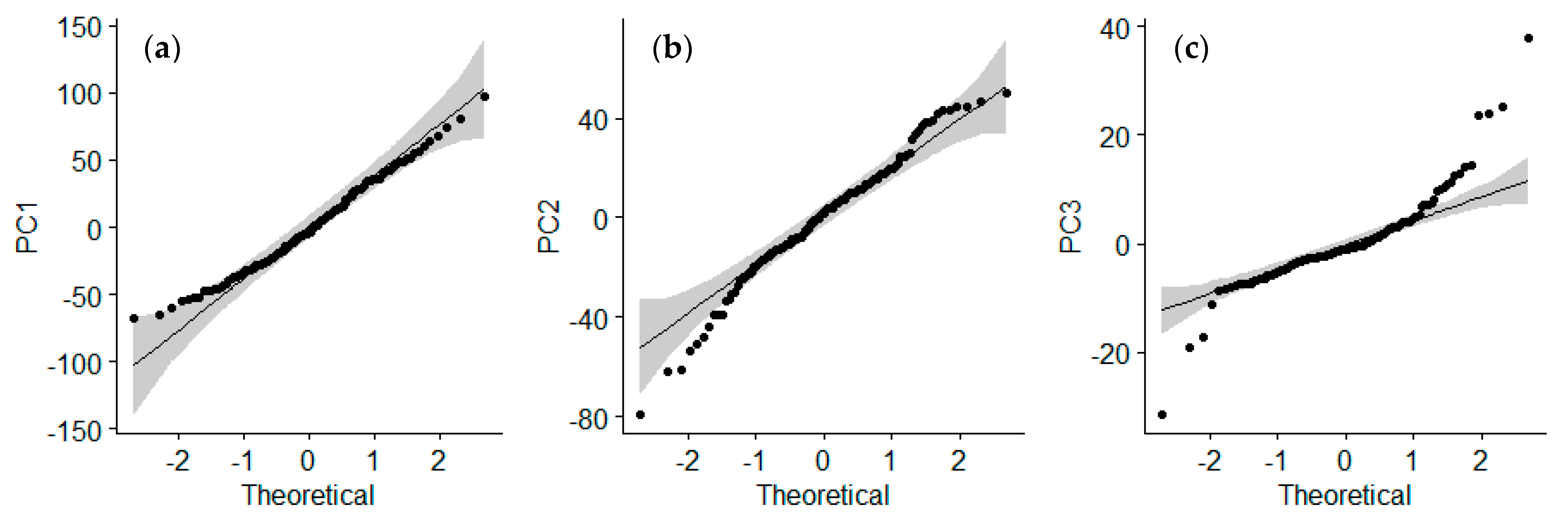
Yield and [Nitrate] average and standard deviation are shown in Table 2, and statistical significance will be provided with the MLM in the 3.3 paragraph.
Exp. B showed the lowest nitrate concentration, which was likely due to the very suitable conditions for the nitrate reductase activity (higher amount of daylight). Chlorosis marks on spinach leaves were observed in Exp. A at harvesting, probably due to the heavy rain registered during the crop cycle and to the consequent hypoxic or anoxic conditions at the root level; this resulted in poorer nitrate discrimination performance, see Section 3.4. Exp. B and C did not show infection or disease marks. In Exp. C, due to emergency issues, two experimental units were not considered in the statistical analysis, resulting in lower Exp. C representation across all trials.

3.2. PCA

The most relevant wavelength regions fall into vis and SWIR for PC1, and NIR for PC2, while PC3 shows only two small peaks in the middle of the green vis area and the red edge sector (Figure 2).
For a better description of the relationship between PCs and the features with which they might correlate a threshold value of 0.80 for the loading values was chosen [40]. The bands exceeding the threshold value for PC1 were (expressed in nm) [450:521], [1310:1349], [1412:1799], and with few excluded λ [2005:2400]. For PC2 were [745:956] and [1016:1123], while PC3 did not provide any loading value above the given threshold value. The first PC1 interval lies between the carotenoid and xanthophyll-responsive bands, at around 450 nm and 530 nm, respectively [41]. The second and third intervals, surrounding the first atmospheric interference band gap, can be considered as a single interval [1310:1799] that includes several C-H and N-H stretch-responsive bands to protein, nitrogen, lignin, and starch content. Similarly, the last interval involves bands related to C-H and N-H rotation, in addition to the ones which are C-O stretch responsive, and they correlate more with protein, cellulose, and nitrogen content [42]. The intervals of PC2 are connected by a small depression around 970 nm followed by a deeper dip at 1200 nm, two regions known to be related to water absorption peaks and responsive to vibrational H-O-H movements [43]. The interval themselves occupy the first two-thirds of the NIR region, well known to be responsive to the structural cell vigor of the leaves [44,45]. Slightly below the threshold, it is worth highlighting that PC1 shows two peaks, in the red and far-red regions, respectively, wherein most of the λ contained in chlorophyll-related VIs fall [45] as well as two bulges (970 nm and 1200 nm) located opposite to the depressions displayed by PC2.
It can be deduced that PC1, accounting for approx. 60% of the sample variability, relates to pigments and structural molecules such as lignin, cellulose, and protein, and secondly to chlorophyll and water content. PC2, which explains 35% of variability, relates principally with vegetative vigor indicators, such as Leaf Area Index (LAI), and secondarily to leaf water content.

3.3. Mixed Linear Models

As a first approach, PCs have been tested against the linearity assumption (Figure 3).
Only PC1 did not appear to differ significantly from the Gaussian bell curve, while PC2 and PC3 need the rank transformation. PC1 and the Gaussian-transformed rPC2 and rPC3 were tested for homoscedasticity against N_fert, by applying Levene’s test (Table 3).
PC1′s variance was comparable to the N_fert factor variance; both rPC2 and rPC3 did not reject the hypothesis of heteroscedasticity.
The variance distribution of the random effects (Table 4) showed that residual variance is prevalent for rPC3, anticipating the low performance of such a model. In PC1 and rPC2 estimation, the most important random factor is GE, followed by N_fert: (GE: block). GE: block factor displayed low importance for all 3 models, indicating the suitability of the randomized block design for all 3 experiments. Significance results for the fixed effects are shown in Table 5; the poorer performance was noticed in the rPC3 model, with statistical significance (95%) only for N_150, N_200, and N_250 treatments.
The PC1 model provided higher significance: 99% for N_100 and N_150 treatments, 95% for N_200 and N_250 treatments, and the rPC2 was the suitable model, showing significance for all the N_fert factor levels.
The higher significance (p-values) that cluster around higher treatments (N_150 to N_250) can easily be explained by the fact that spinach is a crop hungry for nitrogen.
Hence, it can be argued that the GE factor impacts the wavebands correlated with PC1 (vis and SWIR) more than the wavebands correlated with PC2, somehow leaving GE independence to NIR. Thus, reflectance-based predictive methods in spinach, widely applicable as well as resilient to environmental changes and adaptable for technology transfer, could better work if related to variables mostly responsive to the early NIR bands.
The estimation of [Nitrate] in spinach leaves through the MLM showed a pattern similar to the PC1 model with regard to the random effects variance distribution (Table 6). Nevertheless, we registered a higher irrelevance for GE: block effect, while we registered a higher significance of the residual effects; the statistical significance at higher N doses confirmed the behavior of the other models (Table 7).

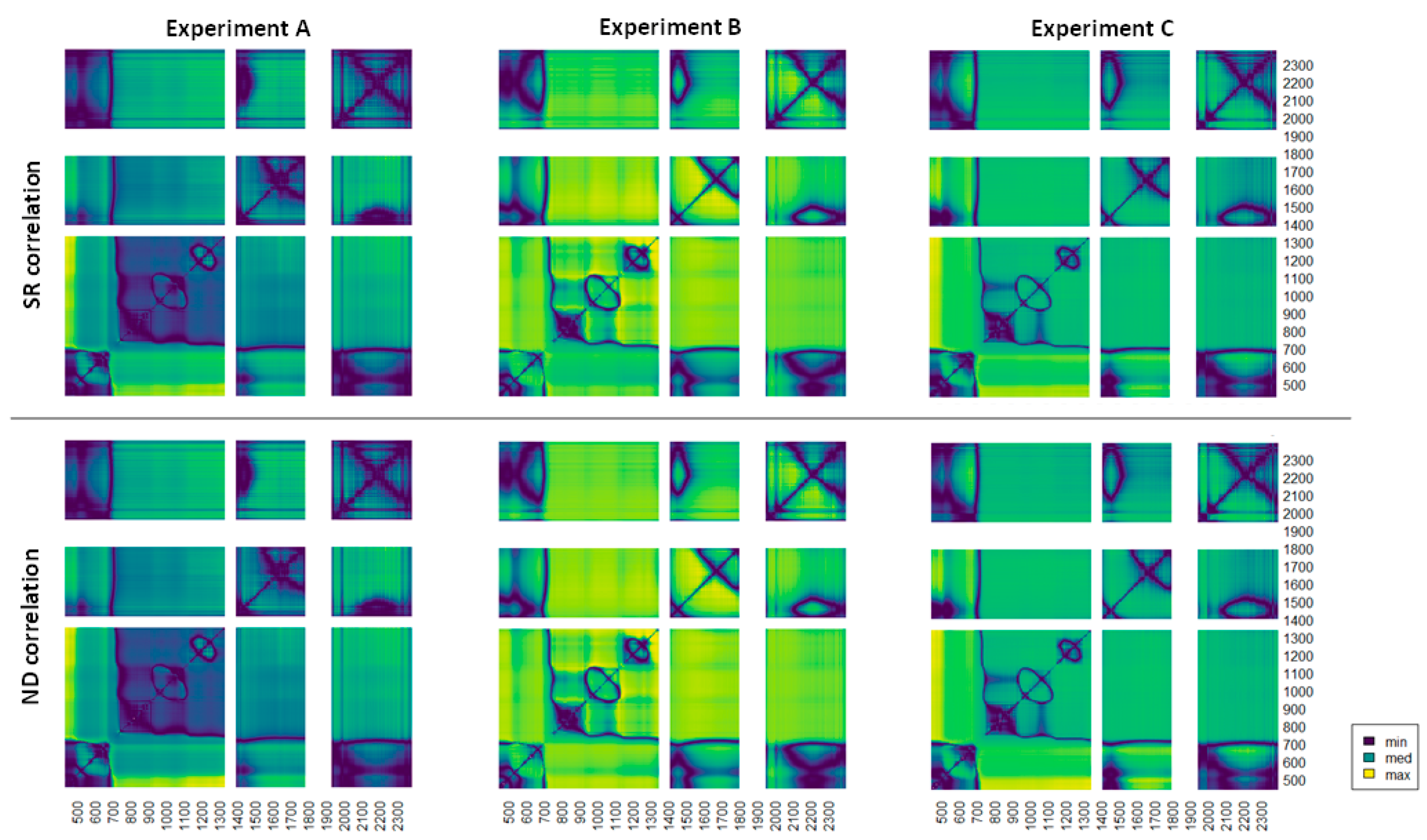
3.4. Wavebands Responsiveness

To individuate the higher responsive spectral bands to the [Nitrate] feature, the heatmaps containing the R2 between all possible SR and ND vs. [Nitrate] from experiments altogether, were released (Figure 4).
Both SR and ND graphs showed a similar pattern with analogous performances. In the literature, there is a lack of comparisons of narrow-band VIs for leaf nitrate content estimation. Although previous findings on nitrogen content confirm the similarity between SR and ND predictive capacity [46]; on the other hand, older comparisons focused on biomass estimation, finding SR to be slightly better than ND [47]. The regions with better performance were the red edge or early NIR (approx. 750:800 nm) in combination with early vis (approx. 400:500 nm), the late NIR (approx. 1100:1300 nm) with the early SWIR (approx. 1450:1600 nm), and the late SWIR with itself (approx. 1700:2200 nm). The SR and ND heatmaps calculated separately for each experiment can provide more in-depth insight, as shown in Figure 5.
Again, both SR and ND graphs showed several similarities across all experiments, though the experiments themselves had varying degrees of accuracy and relevance for the spectral region under consideration. The most accurate and stable in terms of coefficient of determination is the early vis in combination with NIR, which maintained R2 greater than 0.60 in all cases. Looking at the best-performing VIs (see Table 8), it is clear that the narrow bands surrounding 525 nm and 720 nm, as well as 1972 nm and 2270 nm, provide, on average, the most accurate information about [Nitrate]. However, taking into consideration the variability of R2 among the different experiments, the wavebands around 751 nm and 496 nm appeared to be more reliable for providing solid [Nitrate] estimations that can overcome unexpected events (such as the chlorosis insurgence in Exp. A) that alter the accuracy of less robust indexes. Moreover, it is worth highlighting that all predictors also performed against differences in soil cover and canopy architecture, derived by the N_fert gradient provided, and measurable in terms of Leaf Area Index (LAI at harvest: 1.96 and 5.67 for N_0 and N_250, respectively, averaged over all Exp.; data not shown).
In Figure 6, the weighted relative occurrence of each band showed the ones more likely to provide a [Nitrate]-related estimate, wherein the bands around 460 nm, 740 nm, 1150 nm, 1300 nm, and 1972 nm were the most represented. Additionally, apart from the red edge one, no others are closely related to the PC1 or PC2 loadings curve peaks, which seem to rely more on other features to discriminate the crop population, and for that, the PCA alone should not be used to provide an estimate of [Nitrate].

4. Conclusions

The present study demonstrates that it is possible to fine-tune reflectance-based predictors that cope with the challenges posed by a practical technology transfer.
The analysis through MLMs and PCA showed that the GE factor plays a very important role in altering the reflectance properties of the canopy, principally in the vis and SWIR region of the spectrum, affecting the majority of the bands that correlate with specific crop features (such as C-H and N-H bonds), it remains to be investigated if and how the effects of other environmental factors can reshape the reflectance properties.
Nevertheless, a series of accurate VIs for the estimation of nitrate in spinach was calculated and displayed; VIs that associate the early NIR (750:800 nm) with the blue-cyan (400:500 nm) showed very consistent results against GE changes, demonstrating the ability to cope with variability due to soil cover, canopy architecture, genotype, and climatic conditions. The same kind of investigation on other horticultural crops could lead to similar or even better outcomes with great advantages to the production sector. These results provide a useful tool for adopting techniques based on proximal sensing approaches to assess nitrate content in spinach, overcoming the open-field application challenges.

Author Contributions

Conceptualization, A.G. and F.S.; methodology, A.G. and W.P.; software, A.G. and W.P.; formal analysis, W.P., C.P., F.T. and G.S.; investigation, W.P. and A.G.; resources, F.S., G.S. and G.C.; data curation, W.P. and A.G.; writing—original draft preparation, W.P.; writing—review and editing, F.S., W.P., G.C. and A.G.; visualization, F.S., W.P., F.T., C.P., G.S., G.C. and A.G.; supervision, A.G.; project administration, F.S. and G.C.; funding acquisition, F.S. and G.C. All authors have read and agreed to the published version of the manuscript.

Funding

This research was funded by “Ministero dell’agricoltura, della sovranità alimentare e delle foreste (Masaf)”, within the project “AgriDigit”, sub-project “Tecnologie digitali integrate per il rafforzamento sostenibile di produzioni e trasformazioni agroalimentari (AgroFiliere)” [DM 36503.7305.2018 of 20 December 2018].

Data Availability Statement

Data supporting reported results are available, on request, from the corresponding Author.

Acknowledgments

We gratefully acknowledge Maria Assunta Dattoli for her unfathomable help in sampling and data acquisition.

Conflicts of Interest

The authors declare no conflict of interest.

References

  1. Colla, G.; Kim, H.J.; Kyriacou, M.C.; Rouphael, Y. Nitrate in fruits and vegetables. Sci. Hortic. 2018, 237, 221–238. [Google Scholar] [CrossRef]
  2. Santamaria, P.; Gonnella, M.; Elia, A.; Parente, A.; Serio, F. Ways of reducing rocket salad nitrate content. Acta Hortic. 2001, 548, 529–536. [Google Scholar] [CrossRef]
  3. Bian, Z.; Wang, Y.; Zhang, X.; Li, T.; Grundy, S.; Yang, Q.; Cheng, R. A review of environment effects on nitrate accumulation in leafy vegetables grown in controlled environments. Foods 2020, 9, 732. [Google Scholar] [CrossRef]
  4. Kyriacou, M.C.; Soteriou, G.A.; Colla, G.; Rouphael, Y. The occurrence of nitrate and nitrite in Mediterranean fresh salad vegetables and its modulation by preharvest practices and postharvest conditions. Food Chem. 2019, 285, 468–477. [Google Scholar] [CrossRef]
  5. Ranasinghe, R.A.S.N.; Marapana, R.A.U.J. Nitrate and nitrite content of vegetables: A review. J. Pharmacogn. Phytochem. 2018, 7, 322–328. [Google Scholar]
  6. Phillips, W.E.J. Naturally occurring nitrate and nitrite in foods in relation to infant methaemoglobinaemia. Food Chem. Toxicol. 1971, 9, 219–228. [Google Scholar] [CrossRef] [PubMed]
  7. Hmelak Gorenjak, A.; Cencič, A. Nitrate in vegetables and their impact on human health. A review. Acta Aliment. 2013, 42, 158–172. [Google Scholar] [CrossRef]
  8. Jovanovski, E.; Bosco, L.; Khan, K.; Au-Yeung, F.; Ho, H.; Zurbau, A.; Jenkins, A.L.; Vuksan, V. Effect of spinach, a high dietary nitrate source, on arterial stiffness and related hemodynamic measures: A randomized, controlled trial in healthy adults. Clin. Nutr. Res. 2015, 4, 160–167. [Google Scholar] [CrossRef] [Green Version]
  9. Mills, C.E.; Khatri, J.; Maskell, P.; Odongerel, C.; Webb, A.J. It is rocket science–why dietary nitrate is hard to ‘beet’! Part II: Further mechanisms and therapeutic potential of the nitrate-nitrite-NO pathway. Br. J. Clin. Pharmacol. 2017, 83, 140–151. [Google Scholar] [CrossRef] [Green Version]
  10. European Commission. Commission Regulation (EC) No 1258/2011 of 2 December 2011 Amending Regulation (EC) No 1881/2006 as Regards Maximum Levels for Nitrates in Foodstuffs. Off. J. Eur. Union (OJEU) 2011, 320, 15–17. [Google Scholar]
  11. Parks, S.E.; Irving, D.E.; Milham, P.J. A critical evaluation of on-farm rapid tests for measuring nitrate in leafy vegetables. Sci. Hortic. 2012, 134, 1–6. [Google Scholar] [CrossRef]
  12. Muñoz-Huerta, R.F.; Guevara-Gonzalez, R.G.; Contreras-Medina, L.M.; Torres-Pacheco, I.; Prado-Olivarez, J.; Ocampo-Velazquez, R.V. A review of methods for sensing the nitrogen status in plants: Advantages, disadvantages and recent advances. Sensors 2013, 13, 10823–10843. [Google Scholar] [CrossRef] [PubMed]
  13. Loeza Corte, J.M.; Morales Ruiz, A.; Olivar Hernandez, A.; Vargas Ramirez, E.J.; Marin Beltran, M.E.; Leon de la Rocha, J.F.; Hernandez Herrera, P.; Diaz Lopez, E. Effect of nitrogen on agronomic yield, SPAD units and nitrate content in roselle (Hibiscus sabdariffa L.) in dry weather. Int. J. Environ. Agric. Biotech. 2016, 1, 769–776. [Google Scholar]
  14. Zhou, G.; Xinhua, Y. Assessing nitrogen nutritional status, biomass and yield of cotton with NDVI, SPAD and petiole sap nitrate concentration. Exp. Agric. 2018, 54, 531–548. [Google Scholar] [CrossRef]
  15. Yue, X.; Hu, Y.; Zhang, H.; Schmidhalter, U. Evaluation of both SPAD reading and SPAD index on estimating the plant nitrogen status of winter wheat. Int. J. Plant Prod. 2020, 14, 67–75. [Google Scholar]
  16. Galieni, A.; D’Ascenzo, N.; Stagnari, F.; Pagnani, G.; Xie, Q.; Pisante, M. Past and future of plant stress detection: An overview from remote sensing to positron emission tomography. Front. Plant Sci. 2021, 11, 1975. [Google Scholar] [CrossRef]
  17. Torres, I.; Sánchez, M.T.; Pérez-Marín, D. Integrated soluble solid and nitrate content assessment of spinach plants using portable NIRS sensors along the supply chain. Postharvest Biol. Technol. 2020, 168, 111273. [Google Scholar]
  18. Entrenas, J.A.; Pérez-Marín, D.; Torres, I.; Garrido-Varo, A.; Sánchez, M.T. Simultaneous detection of quality and safety in spinach plants using a new generation of NIRS sensors. Postharvest Biol. Technol. 2020, 160, 111026. [Google Scholar] [CrossRef]
  19. Perez-Marin, D.; Torres, I.; Entrenas, J.A.; Vega, M.; Sánchez, M.T. Pre-harvest screening on-vine of spinach quality and safety using NIRS technology. Spectrochim. Acta A Mol. Biomol. Spectrosc. 2019, 207, 242–250. [Google Scholar] [CrossRef]
  20. Mahanti, N.K.; Chakraborty, S.K.; Kotwaliwale, N.; Vishwakarma, A.K. Chemometric strategies for nondestructive and rapid assessment of nitrate content in harvested spinach using Vis-NIR spectroscopy. J. Food Sci. 2020, 85, 3653–3662. [Google Scholar] [CrossRef] [PubMed]
  21. Itoh, H.; Tomita, H.; Uno, Y.; Shiraishi, N. Development of method for non-destructive measurement of nitrate concentration in vegetable leaves by near-infrared spectroscopy. IFAC Proc. Vol. 2011, 44, 1773–1778. [Google Scholar] [CrossRef] [Green Version]
  22. Xue, L.H.; Yang, L.Z. Nondestructive determination of nitrate content in spinach leaves with visible-near infrared high spectra. Spectrosc. Spect. Anal. 2009, 29, 926–930. [Google Scholar]
  23. Sarkar, S.; Jha, P.K. Is precision agriculture worth it? Yes, maybe. J. Biotechnol. Crop Sci. 2020, 9, 4–9. [Google Scholar]
  24. Misara, R.; Verma, D.; Mishra, N.; Rai, S.K.; Mishra, S. Twenty-two years of precision agriculture: A bibliometric review. Precis. Agric. 2022, 23, 2135–2158. [Google Scholar] [CrossRef]
  25. Repubblica Italiana-Ministero delle Politiche Agricole Alimentari e Forestali. Decreto Ministeriale 185 del 13 Settembre 1999. In Approvazione dei “Metodi ufficiali di analisi chimica del suolo”; Gazzetta Ufficiale della Repubblica Italiana—suppl. ord. n.248 del 21 ottobre 1999—Serie generale; Istituto Poligrafico dello Stato: Roma, Italy, 1999. [Google Scholar]
  26. Cataldo, D.A.; Maroon, M.; Schrader, L.E.; Youngs, V.L. Rapid colorimetric determination of nitrate in plant tissue by nitration of salicylic acid. Commun. Soil Sci. Plant Anal. 1975, 6, 71–80. [Google Scholar] [CrossRef]
  27. Morton, F.B.; Altschul, D. Data reduction analyses of animal behaviour: Avoiding Kaiser’s criterion and adopting more robust automated methods. Anim. Behav. 2019, 149, 89–95. [Google Scholar] [CrossRef] [Green Version]
  28. Hair, J.; Anderson, R.E.; Tatham, R.L.; Black, W.C. Exploratory Factor Analysis. In Multivariate Data Analysis, 4th ed.; Hair, J., Anderson, R.E., Tatham, R.L., Black, W.C., Eds.; Prentice-Hall Inc.: Hoboken, NJ, USA, 1995; pp. 94–154. [Google Scholar]
  29. Ghasemi, A.; Zahediasl, S. Normality tests for statistical analysis: A guide for non-statisticians. Int. J. Endocrinol. Metab. 2012, 10, 486. [Google Scholar] [CrossRef] [PubMed]
  30. Oppong, F.B.; Agbedra, S.Y. Assessing univariate and multivariate normality. a guide for non-statisticians. Math. Theory Model. 2016, 6, 26–33. [Google Scholar]
  31. McLean, R.A.; Sanders, W.L.; Stroup, W.W. A unified approach to mixed linear models. Am. Stat. 1991, 45, 54–64. [Google Scholar]
  32. Microsoft Corporation. Microsoft Excel. 2018. Available online: https://office.microsoft.com/excel (accessed on 2 November 2022).
  33. R Core Team. R: A Language and Environment for Statistical Computing; R Foundation for Statistical Computing: Vienna, Austria, 2022; Available online: https://www.R-project.org/ (accessed on 2 November 2022).
  34. Lê, S.; Josse, J.; Husson, F. FactoMineR: An R package for multivariate analysis. J. Stat. Softw. 2008, 25, 1–18. [Google Scholar] [CrossRef] [Green Version]
  35. Kassambara, A.; Mundt, F. Factoextra: Extract and Visualize the Results of Multivariate Data Analyses, R package Version 1.0.7; 2020. Available online: https://CRAN.R-project.org/package=factoextra (accessed on 10 November 2022).
  36. Kassambara, A. Ggpubr: ‘Ggplot2’ Based Publication Ready Plots, R package Version 0.4.0; 2020. Available online: https://CRAN.R-project.org/package=ggpubr (accessed on 10 November 2022).
  37. Bates, D.; Mächler, M.; Bolker, B.; Walker, S. Fitting linear mixed-effects models using lme4. arXiv 2014, arXiv:1406.5823. [Google Scholar]
  38. McCaw, Z. RNOmni: Rank Normal Transformation Omnibus Test, R package Version 1.0.1; 2022. Available online: https://CRAN.R-project.org/package=RNOmni (accessed on 10 November 2022).
  39. Garnier, S.; Ross, N.; Rudis, R.; Camargo, A.P.; Sciaini, M.; Scherer, C. Rvision—Colorblind-Friendly Color Maps for R, R package Version 0.6.2; 2021. Available online: https://sjmgarnier.github.io/viridis/ (accessed on 10 November 2022).
  40. Pane, C.; Galieni, A.; Riefolo, C.; Nicastro, N.; Castrignanò, A. Hyperspectral Reflectance Response of Wild Rocket (Diplotaxis tenuifolia) Baby-Leaf to Bio-Based Disease Resistance Inducers Using a Linear Mixed Effect Model. Plants 2021, 10, 2575. [Google Scholar] [CrossRef]
  41. Peñuelas, J.; Filella, I. Visible and near-infrared reflectance techniques for diagnosing plant physiological status. Trends Plant Sci. 1998, 3, 151–156. [Google Scholar] [CrossRef]
  42. Berger, K.; Verrelst, J.; Feret, J.B.; Wang, Z.; Wocher, M.; Strathmann, M.; Danner, M.; Mauser, W.; Hank, T. Crop nitrogen monitoring: Recent progress and principal developments in the context of imaging spectroscopy missions. Remote Sens. Environ. 2020, 242, 111758. [Google Scholar] [CrossRef] [PubMed]
  43. Walrafen, G.E.; Pugh, E. Raman Combinations and Stretching Overtones from Water, Heavy Water, and NaCl in Water at Shifts to ca. 7000 cm−1. J. Solut. Chem. 2004, 33, 81–97. [Google Scholar] [CrossRef]
  44. Rouse, J.W. Monitoring vegetation systems in the Great Plains with Earth Resources Technology (ERTS) Satellite. In Proceedings of the 3rd Earth Resources Technology Satellite Symposium, Washington, DC, USA, 10–14 December 1973. [Google Scholar]
  45. Verma, B.; Prasad, R.; Srivastava, P.K.; Yadav, S.A.; Singh, P.; Singh, R.K. Investigation of optimal vegetation indices for retrieval of leaf chlorophyll and leaf area index using enhanced learning algorithms. Comput. Electron. Agric. 2022, 192, 106581. [Google Scholar] [CrossRef]
  46. Friedel, M.; Hendgen, M.; Stoll, M.; Löhnertz, O. Performance of reflectance indices and of a handheld device for estimating in-field the nitrogen status of grapevine leaves. Aust. J. Grape Wine Res. 2020, 26, 110–120. [Google Scholar] [CrossRef] [Green Version]
  47. Mutanga, O.; Skidmore, A.K. Narrow band vegetation indices overcome the saturation problem in biomass estimation. Int. J. Remote Sens. 2004, 25, 3999–4014. [Google Scholar] [CrossRef]
Figure 1. Thermo-pluviometric conditions during Exp. A, B, and C. Brown line represents the 10 days average temperature in degrees Celsius (left Y axis), and blue bars are the total rain registered every 10 days in mm (right Y axis). Semi-transparent boxes cover the time (X axis) from sowing to harvesting for each experiment: red, green, and yellow for Exp. A, B, and C, respectively.
Agronomy 13 00193 g001
Figure 2. Graph of the loading values for PC1 (blue dots), PC2 (red dots), and PC3 (grey dots). The dashed horizontal line represents the chosen threshold, and the grey boxes are the bands wherein reflectance data have been omitted from the database, because of significant atmospheric effects. Arrows and braces indicate in which spectrum location there are known relationships with the presented features. For clarity, the entire graph, where the loadings axis span from −1 to 1, is represented inside the box in the bottom right corner.
Agronomy 13 00193 g002
Figure 3. Quantile-Quantile plots for PC1 (a), PC2 (b), and PC3 (c). The black line represents a perfectly normal distribution, the shaded grey shape represents the 95% confidence interval within the real distribution (Black dots) should stay.
Agronomy 13 00193 g003
Figure 4. Coefficient of determination Heatmaps between calculated vegetation indices (VIs) (both Simple Ratios, SR, and Normalized Difference, ND) vs. nitrate content ([Nitrate]) for the entire dataset (including Exp. A, Exp. B, and Exp. C; see Table 1 for further details). White bands correspond to the bands which have been removed from the database, because of significant atmospheric effects.
Agronomy 13 00193 g004
Figure 5. Coefficient of determination Heatmaps between calculated vegetation indices (VIs) (both Simple Ratios, SR, and Normalized Difference, ND) vs. nitrate content ([Nitrate]) for each experiment (Exp. A, Exp. B, and Exp. C; see Table 1 for further details). White bands correspond to the bands which have been removed from the database because of significant atmospheric effects.
Agronomy 13 00193 g005
Figure 6. Weighted wavelength occurrence on nitrate content ([Nitrate]) estimation. Black line: occurrence frequency, in best-performing Vegetation Indexes (VIs), listed in Table 7, weighted by produced R2 (coefficient of determination) in the [Nitrate] estimation (ordinate axis), of wavelength bands (abscissa axis express as nm)—width calculated concerning instrumental spectrum resolution (see Section 2.2). For clarity, in the same graph, PC1 and PC2 highest loading values (threshold above 0.5) are represented in blue and red, respectively.
Agronomy 13 00193 g006
Table 1. Details of the three experimental fields.
Field CoordinatesGenotypeSowing DateHarvest Date
Exp. A42°47′50″ N
13°47′02″ E
Bufflehead—Rijk Zwaan24 October 202026 January 2021
Exp. B42°47′54″ N
13°48′06″ E
Monterey F1—Cora Seeds22 January 20215 May 2021
Exp. C42°48′08″ N
13°46′49″ E
Kangaroo RZ F1—Rijk Zwaan15 October 202127 January 2022
Table 2. Yield (g m−2) and Nitrate content ([Nitrate]; mg kg−1 dry weight, DW) as recorded for spinach subjected to different N availabilities (0, 50, 100, 150, 200, and 250 kg N ha−1: N_0, N_50, N_100, N_150, N_200, and N_250, respectively) in 3 different experiments (Exp. A, B, and C) during 2020–2022 (see Table 1). Data are expressed as treatment average ± standard deviation.
TreatmentYield (g m−2) Fresh Weight[Nitrate]
(mg kg−1 DW)
Exp. AN_01467 ± 631219 ± 152
N_502035 ± 227932 ± 161
N_1002452 ± 211513 ± 146
N_1502852 ± 3332185 ± 633
N_2003554 ± 2863368 ± 268
N_2503555 ± 1984885 ± 344
Exp. BN_01160 ± 113732 ± 68
N_502313 ± 862789 ± 38
N_1002699 ± 471790 ± 91
N_1502749 ± 4101214 ± 250
N_2004440 ± 5472419 ± 626
N_2504412 ± 4912457 ± 237
Exp. CN_01253 ± 611142 ± 60
N_501616 ± 971089 ± 20
N_1002893 ± 2081577 ± 90
N_1503497 ± 2001809 ± 57
N_2004445 ± 1283489 ± 47
N_2504087 ± 3394147 ± 133
Table 3. Levene’s test for homoscedasticity against N fertilization. rPC2 and rPC3 are ranked (Gaussian) transformations of PC2 and PC3. Degrees of Freedom are 135 for all 3 variables. Significance codes: p-value < 0.001 ***, p-value < 0.05 *.
Levene’s TestPC1rPC2rPC3
F value1.04774.79622.3938
p-value3.92 × 10−14.56 × 10⁻⁴ ***4.08 × 10⁻² *
Table 4. Random effects variance, variance standard deviation, and percentage of total variance for each mixed linear model estimating PC1, rPC2, and rPC3, respectively. N_fert: N fertilization treatments; GE: genotype × environment.
Random EffectsPC1rPC2rPC3
VarianceSt. DevVariance %VarianceSt. DevVariance %VarianceSt. DevVariance %
N_fert: (GE: block)318.817.825.0%0.18370.428627.7%0.277217.828.7%
GE: block153.212.412.0%0.08830.297213.3%0.141112.414.6%
GE550.223.543.2%0.21950.468533.1%0.092323.59.6%
Residual250.915.819.7%0.17090.413425.8%0.455215.847.1%
Table 5. Fixed effect results and significance in the estimation of the PCs loading values. Significance codes: p-value < 0.001 ***, p-value < 0.01 **, p-value < 0.05 *. N_0, N_50, N_100, N_150, N_200, and N_250: treatments fertilized with 0, 50, 100, 150, 200, and 250 kg N ha−1, respectively.
Fixed EffectsPC1rPC2rPC3
t-Valuep-Valuet-Valuep-Valuet-Valuep-Value
N_01.432.44 × 10−1−3.09* 4.16 × 10−21.919.32 × 10−2
N_50−1.252.20 × 10−12.46* 1.88 × 10−2−1.551.29 × 10−1
N_100−3.41** 1.68 × 10−33.53** 1.17 × 10⁻³−1.621.14 × 10−1
N_150−2.99** 5.09 × 10−34.31*** 1.21 × 10⁻⁴−2.34* 2.49 × 10−2
N_200−2.15* 3.90 × 10−26.60*** 1.23 × 10⁻⁷−2.44* 2.00 × 10−2
N_250−2.56* 1.49 × 10−25.97*** 8.06 × 10⁻⁷−2.54* 1.57 × 10−2
Table 6. Random effects variance, variance standard deviation, and percentage of total variance for the mixed linear model estimating nitrate content ([Nitrate]) in spinach leaves. N_fert: N fertilization treatments; GE: genotype × environment.
Random Effects[Nitrate]
VarianceSt. DevVariance %
N_fert: (GE)0.08750.29623.3%
GE: block0.01740.1324.63%
GE0.1650.40744.0%
Residual0.1060.32528.1%
Table 7. Fixed effect results and significance in the estimation of the nitrate content ([Nitrate]) in spinach leaves subjected to different N fertilization (0, 50, 100, 150, 200, and 250 kg N ha−1: N_0, N_50, N_100, N_150, N_200, and N_250, respectively). Significance codes: p-value < 0.001 ***, p-value < 0.05 *.
Fixed Effects[Nitrate]
t-Valuep-Value
N_0−2.40 × 1005.1 × 10−2
N_50−1.28 × 1002.2 × 10−1
N_1006.22 × 10−15.4 × 10⁻¹
N_1502.72 × 100* 1.5 × 10−2
N_2005.25 × 100*** 8.7 × 10⁻⁵
N_2507.62 × 100*** 1.0 × 10⁻⁶
Table 8. Best-performing Vegetation Indexes (VIs) for the coefficient of determination (R2) with nitrate content ([Nitrate]) in spinach leaves, as recorded in Exp. A, Exp. B, and Exp. C (see Table 1 for further details) as well as Exp. A+B+C altogether (grey background). Numbers refer to reflectance at wavelength expressed in nm; vis, NIR, and SWIR refer to the spectral zones ranging from 450:750 nm, 751:1349 nm, and 1411:2400 nm, respectively.
Exp. Equation (Reflectance [nm])R2Exp.Spectrum ZoneEquation (Reflectance [nm])R2
Simple RatioAvis-vis465/7350.57Cvis-vis460/7400.77
vis-NIR + NIR-vis463/13500.63vis-NIR + NIR-vis460/13500.82
NIR-NIR1198/12590.47NIR-NIR1150/11570.67
vis-SWIR + SWIR-vis435/16320.50vis-SWIR + SWIR-vis494/16520.76
NIR-SWIR + SWIR-NIR2298/13450.52NIR-SWIR + SWIR-NIR1300/19740.62
SWIR-SWIR1972/14370.56SWIR-SWIR1979/20300.74
Bvis-vis454/7400.77A + B + Cvis-vis525/7200.69
vis-NIR + NIR-vis454/12400.77vis-NIR + NIR-vis496/7510.64
NIR-NIR1301/12940.83NIR-NIR1318/11650.56
vis-SWIR + SWIR-vis745/15220.76vis-SWIR + SWIR-vis740/19700.65
NIR-SWIR + SWIR-NIR1289/15680.79NIR-SWIR + SWIR-NIR1165/19700.65
SWIR-SWIR1593/15700.83SWIR-SWIR1972/22700.68
Normalized DifferenceAvis-vis(732 + 463)/(732 − 463)0.57Cvis − vis(740 + 460)/(740 − 460)0.77
vis-NIR + NIR-vis(1350 + 463)/(1350 − 463)0.63vis − NIR + NIR − vis(1350 + 460)/(1350 − 460)0.81
NIR-NIR(1259 + 1198)/(1259 − 1198)0.46NIR − NIR(1150 + 1157)/(1150 − 1157)0.67
vis-SWIR + SWIR-vis(495 + 1632)/(495 − 1632)0.50vis − SWIR + SWIR − vis(494 + 1640)/(494 − 1640)0.75
NIR-SWIR + SWIR-NIR(1338 + 2297)/(1338 − 2297)0.52NIR − SWIR + SWIR − NIR(1120 + 2397)/(1120 − 2397)0.60
SWIR-SWIR(2297 + 1800)/(2297 − 1800)0.56SWIR − SWIR(2030 + 1979)/(2030 − 1979)0.73
Bvis-vis(740 + 454)/(740 − 454)0.77A + B + Cvis − vis(722 + 525)/(722 − 525)0.69
vis-NIR + NIR-vis(454 + 1240)/(454 −1240)0.77vis − NIR + NIR − vis(751 + 496)/(751 − 496)0.65
NIR-NIR(1301 + 1294)/(1301 − 1294)0.83NIR − NIR(1318 + 1165)/(1318 − 1165)0.57
vis-SWIR + SWIR-vis(1570 + 750)/(1570 − 750)0.74vis − SWIR + SWIR − vis(740 + 1972)/(740 − 1972)0.60
NIR-SWIR + SWIR-NIR(1289 + 1570)/(1289 − 1570)0.77NIR − SWIR + SWIR − NIR(1349 + 1972)/(1349 − 1972)0.62
SWIR-SWIR(1593 + 1570)/(1593 −1570)0.83SWIR − SWIR(2270 + 1972)/(2270 − 1972)0.68
Disclaimer/Publisher’s Note: The statements, opinions and data contained in all publications are solely those of the individual author(s) and contributor(s) and not of MDPI and/or the editor(s). MDPI and/or the editor(s) disclaim responsibility for any injury to people or property resulting from any ideas, methods, instructions or products referred to in the content.

