A Cotton Leaf Water Potential Prediction Model Based on Particle Swarm Optimisation of the LS-SVM Model

Abstract

Frequent monitoring of crop moisture levels can significantly improve crop production efficiency and optimise water resource utilisation. The aim of the present study was to generate moisture status maps using thermal infrared imagery, centring on the development of a predictive model for the cotton leaf water potential. The model was constructed using particle swarm optimisation (PSO) in conjunction with the least squares support vector machine (LS-SVM). Traditional SVM models suffer from high computational complexity, long training times, and inequality constraints in predicting leaf water potential. To address such issues, the PSO algorithm was introduced to improve the performance of the LS-SVM model. The PSO-optimised LS-SVM model exhibited notable improvements in performance when evaluated on two distinct test datasets (Alaer and Tumushuke). The research results indicate that the predictive accuracy of the PSO-LS-SVM model significantly improved, as evidenced by an increase of 0.05 and 0.04 in the $R^2$ values, both of which reached 0.95. This improvement is reflected in the corresponding RMSE values, which were reduced to 0.100 and 0.103. Furthermore, a model was established based on data from three cotton growth stages, achieving high predictive accuracy even with fewer training samples. By using the PSO-LS-SVM model to predict leaf water potential information, the predicted data were mapped onto drone images, enabling the transformation of the leaf water potential from a point to an area. The present findings contribute to a more comprehensive understanding of the cotton leaf water potential by visually representing the spatial distribution of crop water status on a large scale. The results hold substantial significance for the improvement of crop irrigation management.

1. Introduction

Thermal infrared crop sensing technology holds the potential for monitoring and mapping the crop moisture status [1,2,3]. Due to the growing affordability of thermal sensors and imaging devices, researchers have been exploring diverse platforms to acquire canopy temperature data at both the canopy and field scales, with the goal of generating maps that depict changes in moisture status. Cohen et al. [4] and Alchanatis et al. [5] employed thermal cameras mounted on elevated cranes to assess the cotton canopy moisture status under different irrigation regimes. The results indicated an inverse relationship between the empirical and theoretical Crop Water Stress Index (CWSI) and leaf water potential (LWP). To create LWP maps based on the CWSI, a reliable relationship between the two metrics needs to be established for different crops and growth stages. As mentioned earlier, prior research has shown correlations between these metrics across various crops. However, most studies have presented results for individual dates [6,7,8]. Certain investigations examining the correlation between the CWSI and LWP in cotton have utilised data collected from multiple dates throughout a season, consistently revealing a relatively stable relationship between the two variables [9,10]. While exploring irrigation scheduling in pumpkin seeds, Kirnak et al. [11] identified noteworthy correlations among an increasing CWSI, decreasing leaf water potential, and various parameters such as the LWP values, seed yield, and leaf area index (LAI) as well as the oil and protein content. The aim of the present study was to analyse cotton across different growth seasons and geographical regions to determine whether a robust relationship exists between the cotton LWP and CWSI based on high-resolution ground-based thermal infrared imagery.

Using thermal infrared images collected by unmanned aerial vehicles (UAVs), Cohen et al. [12] calculated the CWSI for predicting the LWP. The results demonstrated the effectiveness of the CWSI in predicting the cotton crop moisture status, revealing the potential for real-time irrigation scheduling. Utilizing terahertz radiation spectroscopy, Browne et al. [13] predicted the leaf water potential and relative water content, highlighting the significance of terahertz radiation in assessing the leaf moisture status within the range of leaf dehydration, which is crucial for controlling gas exchange and leaf survival. Cohen et al. [4] predicted the leaf water potential through an empirical formula based on the crop canopy temperature and CWSI. By integrating the CWSI, temperature, and wind speed, a multivariate regression model was established that exhibited enhanced prediction accuracy for the leaf water potential. Ultimately, statistical analysis revealed a relatively stable relationship between the crop moisture status indicator, CWSI, and leaf water potential, with a correlation coefficient slightly higher than that between the canopy temperature and leaf water potential.

In the present study, a novel method for estimating the leaf water potential is proposed. A cotton leaf water potential prediction model is established based on multi-source data using the least squares support vector machine (LS-SVM) model. To achieve improved data transfer and processing efficiency in this model, Kernel function types and regularisation parameters are defined. To enhance the performance of the LS-SVM model, the particle swarm optimisation (PSO) algorithm is introduced so as to allow for the searching of optimal parameters, as well as the optimisation of the particle update scale and velocity for increased prediction accuracy and generalisation capability. Furthermore, a prediction model based on the PSO-LS-SVM model is established. Finally, spatiotemporal distribution maps of the leaf water potential were generated based on the leaf water potential prediction model. With limited ground-based biophysical measurements, the crop moisture status is displayed using high-resolution imagery.

2. Materials and Methods

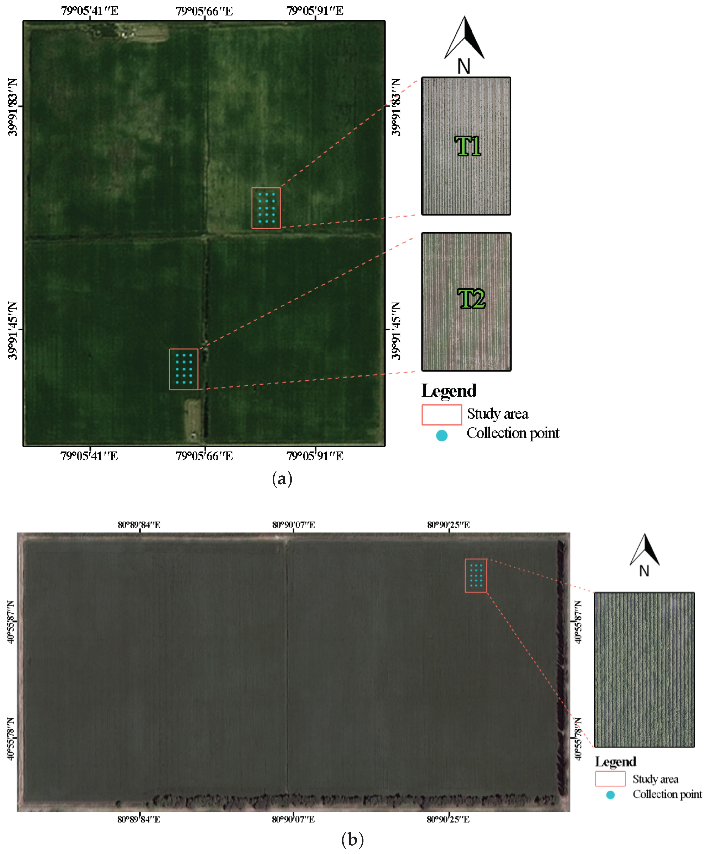
2.1. Site Description and Experimental Design

The experiments were conducted in Tumushuke and Alaer (Figure 1), Xinjiang, China during the years 2022 and 2023. The Tumushuke test site is located at the coordinates ${79}^{\circ }{05}^{\prime }{66}^{″}$ E, ${39}^{\circ }{91}^{\prime }{45}^{″}$ N with an altitude of 1046.25 m. The annual average precipitation is 38.3 mm, the average annual evaporation is 2030.8 mm, and the annual sunshine hours amount to 2923.7 h. The average annual temperature is 11.6 °C, and the frost-free period spans 225 days. The Alaer test site is located at the coordinates ${80}^{\circ }{90}^{\prime }{36}^{″}$ E, ${40}^{\circ }{59}^{\prime }{66}^{″}$ N with an altitude of 1014.12 m. It receives approximately 2996.2 h of sunshine annually, annual average precipitation of 40.1 mm, and annual evaporation of 1976.6 mm. Both locations are characterised by intense solar radiation, significant day-night temperature fluctuations, and sandy loam soil, making them conducive for the cultivation of a variety of crops, with a particular suitability for cotton.

Data for the year 2022 were collected from Tumushuke twice a week, while data for 2023 were collected from both Tumushuke and Alaer twice a month from the flowering period to the end of the open boll period. Dry sowing and wet seedling transplantation techniques were employed in both locations, with planting taking place in early April. Cotton was planted in a configuration of 1 row, 6 rows, and 3 pipes with a film width of 2.05 m, using the mechanical cotton planting mode with row spacing of 66 + 10 + 66 + 10 cm. The first irrigation was conducted in early June. In the Tumushuke test area, two plots (T1 and T2) were established, while one plot was established in the Alaer test area. Each plot covered an area of 50 m by 30 m, with a sampling point positioned every 5 m along the perimeter. To aid precise drone positioning, coloured cardboard sheets were placed at each sampling point to serve as visual markers for the drone.

2.2. Unmanned Aerial Vehicle Thermal Infrared Image Acquisition

An unmanned aerial vehicle system (Mavic 2 Enterprise Advanced, manufactured by DJI) was utilised to simultaneously capture high-resolution visible light and thermal infrared images. The visible light camera has a resolution of 48 million pixels and an equivalent focal length of 24 mm. The thermal infrared camera operates within a wavelength range of 8–14 μm, with a sensor resolution of 640 × 512 pixels and a lens focal length of 9 mm. The temperature measurement accuracy is ±2 °C. The flights were conducted at an altitude of 50 m with a spatial resolution of 0.9 cm. The DJI Thermal Analysis Tool was employed to extract the cotton canopy temperatures at the sampling points.

2.3. Ground Data Collection

2.3.1. Meteorological Data

In the experimental areas, standard meteorological stations were installed to automatically record various meteorological parameters throughout the crop’s growth period. These stations collected data at hourly intervals, including the temperature, wind speed, rainfall, solar radiation, atmospheric humidity, and atmospheric pressure.

2.3.2. Soil Moisture Content

The soil moisture content was measured using a soil moisture meter (TDR350, manufactured by Spectrum Technologies) with the probe length set at 20 cm. Drip-irrigated cotton exhibits distinct characteristics compared with conventional furrow-irrigated cotton primarily because its root system tends to be relatively shallow, with a primary concentration at a depth of approximately 20 cm. The data collected for the present study encompassed various parameters, including the soil volumetric moisture content, soil temperature, soil electrical conductivity (EC), and GPS coordinates among other relevant factors.

2.3.3. Leaf Water Potential

Leaf water potential measurements were conducted concurrently with the unmanned aerial vehicle capture of thermal infrared images of the crop canopy. These measurements and image capture occurred at 2:00 p.m. local time. Fifteen healthy and well-developed mature leaves from the experimental plots were selected for measurement. Prior to measurement, aluminium foil bags were used to encase the leaves for approximately 30 min, allowing for the equilibration of water conductance between the leaves and adjacent branches [14]. The leaf water potential was determined using a plant water potential pressure chamber (QT-WP080A, manufactured by Qudaotech).

2.4. Processing Unmanned Aerial Vehicle Imagery

The acquisition of cotton field remote sensing images via the unmanned aerial vehicle remote sensing system necessitated image preprocessing to generate essential data that could be used for subsequent research purposes. Firstly, the UAV remote sensing images and corresponding GPS information were imported into Pix4DMapper (Pix4D Inc., Prilly, Switzerland). Lens distortion correction was performed based on the infrared camera’s focal length and lens centre point. To accurately locate the captured points in the cotton canopy, the scale-invariant feature transform (SIFT) algorithm was utilised to align the visible light and thermal infrared images. The SIFT features and descriptors were extracted from both images. By matching these feature points, a correspondence relationship between the two images was established, identifying common points between the visible light and thermal infrared images. Subsequently, the random sample consensus (RANSAC) algorithm was employed to estimate the transformation matrix, aligning the visible light image with the thermal infrared image. The computation of the CWSI required pure canopy pixels, necessitating the removal of soil pixels from the unmanned aerial vehicle’s thermal infrared images. However, traditional methods for soil background removal are complex and costly [15]. To overcome the described issue, the Canny edge detection algorithm in OpenCV was utilised to extract the edges of the cotton canopy from the thermal infrared images, resulting in raster images featuring the edge characteristics of the cotton canopy. Subsequently, these edge raster images were transformed into cotton canopy vector layers using ArcGIS. Finally, these vector layers were used to clip the unmanned aerial vehicle thermal images, effectively removing soil pixels from the images.

2.5. Unmanned Aerial Vehicle Thermal Infrared Image Temperature Correction Analysis

To enhance the application of unmanned aerial vehicle thermal infrared remote sensing technology in field cotton water stress monitoring, temperature correction of the thermal infrared images is essential. A common approach involves establishing a linear regression model between handheld infrared thermometers and measurements from unmanned aerial vehicle thermal infrared images [16]. In the present study, prior to field image acquisition, the UAV obtained images of standard panels with 25% and 75% reflectance as well as images of water bodies from an altitude of 50 m. Water bodies are typically considered relatively stable temperature sources, especially under relatively constant environmental conditions. By placing ice bags on the water body to lower its temperature, a known low-temperature point was created. Using a handheld thermometer, the water temperatures were measured as reference temperatures. By comparing the reference temperatures with the corresponding pixel temperatures on the thermal infrared images, the infrared temperature images were calibrated, resulting in the generation of more precise and accurate temperature values for the thermal infrared images captured by the unmanned aerial vehicle.

2.6. Calculation of the Crop Water Stress Index

To better visualise the spatial and temporal distribution of cotton water stress conditions and map them onto the thermal infrared images from the unmanned aerial vehicle, a simplified method was employed for calculating the CWSI, as referenced from the work of J. Bian et al. [17]. This method is based on the crop canopy temperature histogram of the entire experimental area and is calculated using the following formula:

$$CWSI=\frac{T_C-T_{wet}}{T_{dry}-T_{wet}}$$

(1)

where the following definitions apply:

• T${}_C$ is the canopy temperature of the cotton, in °C.
• T${}_{wet}$ is the average temperature of the lowest 5% of the temperature histogram in °C.
• T${}_{dry}$ is the average temperature of the highest 5% of the temperature histogram in °C.

This simplified method allows for the calculation of the CWSI, enabling the monitoring of water stress levels in cotton and their spatial–temporal distribution.

2.7. Establishment and Parameter Optimisation of the LS-SVM Leaf Water Potential Prediction Model

Experimental data from 2022 to 2023 were utilised in the present study, comprising a total of 510 datasets for modelling. A random selection was made of 300 data sets collected in 2022, which were designated as the training samples. The remaining 120 data sets obtained in 2022 were set aside for use as validation samples. Additionally, 45 data sets from both Alaer and Tumushuke collected in 2023 were employed as test samples. To further validate the robustness and generalisation capability of the proposed leaf water potential prediction model across different years, the training and test sets were redefined based on the cotton growth stages. Specifically, 100 data sets from the flowering and full boll stages and 115 data sets from the open boll stages of cotton in 2022 were used as the training set, while the remaining 50 data sets from the same stages in 2022 were allocated to the validation set. Furthermore, 15 data sets from the flowering, full boll, and open boll stages of cotton in the work of Alaer and Tumushuke in 2023 were selected as the test set. The goal was to investigate whether the model could adapt to varying growth conditions across different years and provide accurate predictions when faced with new and distinct circumstances.

The model employed eight factors as input variables: cotton canopy temperature, soil volumetric moisture content, soil temperature, atmospheric temperature, atmospheric humidity, light intensity, photosynthetically active radiation, and atmospheric pressure. The leaf water potential served as the output variable. To ensure the model’s robustness, data normalisation was applied by employing the min-max normalisation method, which is suitable for various data distributions and contributes to enhancing the convergence speed and performance of the model, and both the LS-SVM and PSO-LS-SVM crop leaf water potential prediction models were established.

The LS-SVM is a machine learning method employed for tasks like pattern classification and regression [18,19]. It trains support vector machine models by applying the least squares method to minimise the loss function. However, the LS-SVM model demands meticulous tuning of the hyperparameters to achieve optimal performance and the selection of appropriate kernel functions tailored to specific problem types. When dealing with large datasets, the computational complexity of the LS-SVM may become a challenge. Moreover, when sample sizes are limited, the LS-SVM can be prone to overfitting, necessitating the use of regularisation techniques to enhance its generalisation performance.

The PSO-LS-SVM approach presents several advantages in terms of hyperparameter optimisation, kernel function selection, and generalisation performance. PSO automates the search in the hyperparameter space, which aids in discovering improved parameter configurations and reduces the need for manual tuning. Additionally, PSO can provide more effective strategies for selecting kernel functions while adapting to various data characteristics. When compared with other machine learning algorithms and prediction models such as extra trees, SVM, and XGBoost [20,21,22], the PSO-LS-SVM algorithm exhibited superior predictive performance, particularly on smaller datasets [23]. This is due to the stronger generalisation ability of support vector machines, which cope better with small sample problems. In parallel, PSO’s global optimisation capability avoids the issue of artificial neural networks getting trapped in local optima during parameter optimisation. Cotton’s water status can be categorised into five stages based on the magnitude of the leaf water potential values [24], as shown in

Table 1. Water status classification of cotton leaf water potential.

Class	LWP Range (MPa)	Water Status Description
1	LWP > [−1.45]	Over-irrigated plants (Oir)
2	−1.45 ≥ LWP > −1.75	Well-watered plants (WW)
3	−1.75 ≥ LWP > −2.05	Low water stress (LWS)
4	−2.05 ≥ LWP > −2.35	Medium water stress (MWS)
5	−2.35 ≥ LWP	Severe water stress (SWS)

.

In the present study, both the LS-SVM and PSO-LS-SVM models were implemented with a radial basis kernel function. For the PSO-LS-SVM model, the following parameters were selected: a population size of M = 30, an inertia weight of w = 0.9, learning factors c₁ = c₂ = 2, a swarm size set to 30, regularisation parameter $\gamma$ = 300, kernel parameter ${\sigma }^2$ = 0.2, and a maximum iteration count for PSO of 50.

3. Results

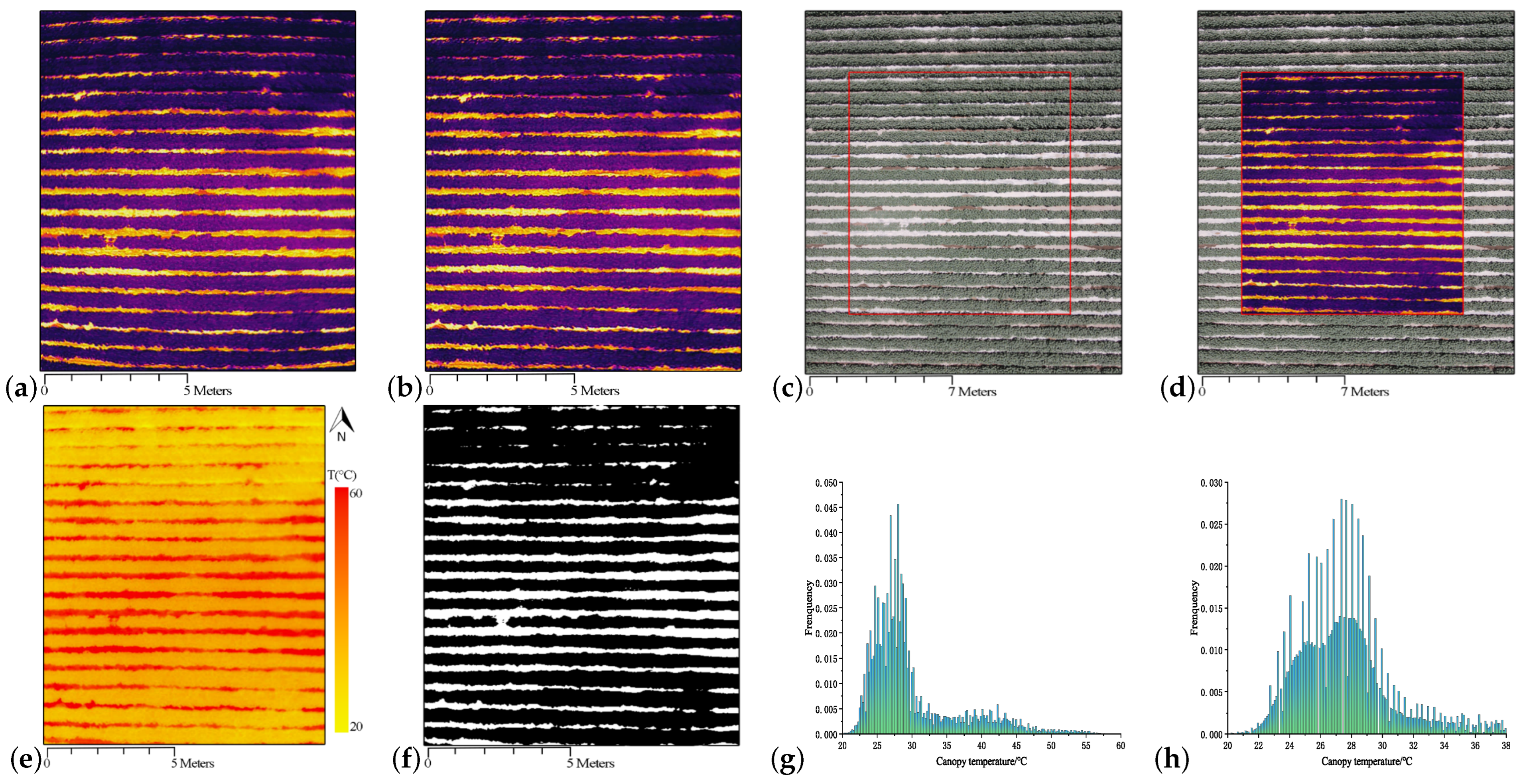
3.1. Impact of the Soil Background on the Cotton Canopy Temperature

Figure 2a shows the original thermal infrared image captured by the drone, while Figure 2b displays the thermal infrared image after lens distortion correction. The Structural Similarity Index (SSIM) between the uncorrected thermal infrared image and the visible light image was 0.2092, whereas the SSIM between the corrected thermal infrared image and visible light image increased to 0.3598. This significantly increased SSIM value indicates that during the correction process, the details and structure of the thermal infrared image were improved, making it closer to the features of the visible light image and thereby improving the overall quality and usability of the image. The cotton canopy mask obtained using the Canny edge detection algorithm is depicted in Figure 2f. After removing the soil background from the thermal infrared image of the cotton canopy, a distinct temperature histogram different from the previous one was obtained. Before soil background removal, the temperature histogram displayed a relatively wide temperature range (20–60 °C), as shown in Figure 2g. The wide temperature range likely included temperature data from both the cotton plants and the adjacent soil, posing a challenge in accurately distinguishing the actual temperature distribution of the plants. However, following the removal of the soil background, the temperature histogram’s range significantly decreased to 20–38 °C, as depicted in Figure 2h. Such a noticeable difference indicates the successful elimination of temperature interference from the soil background.

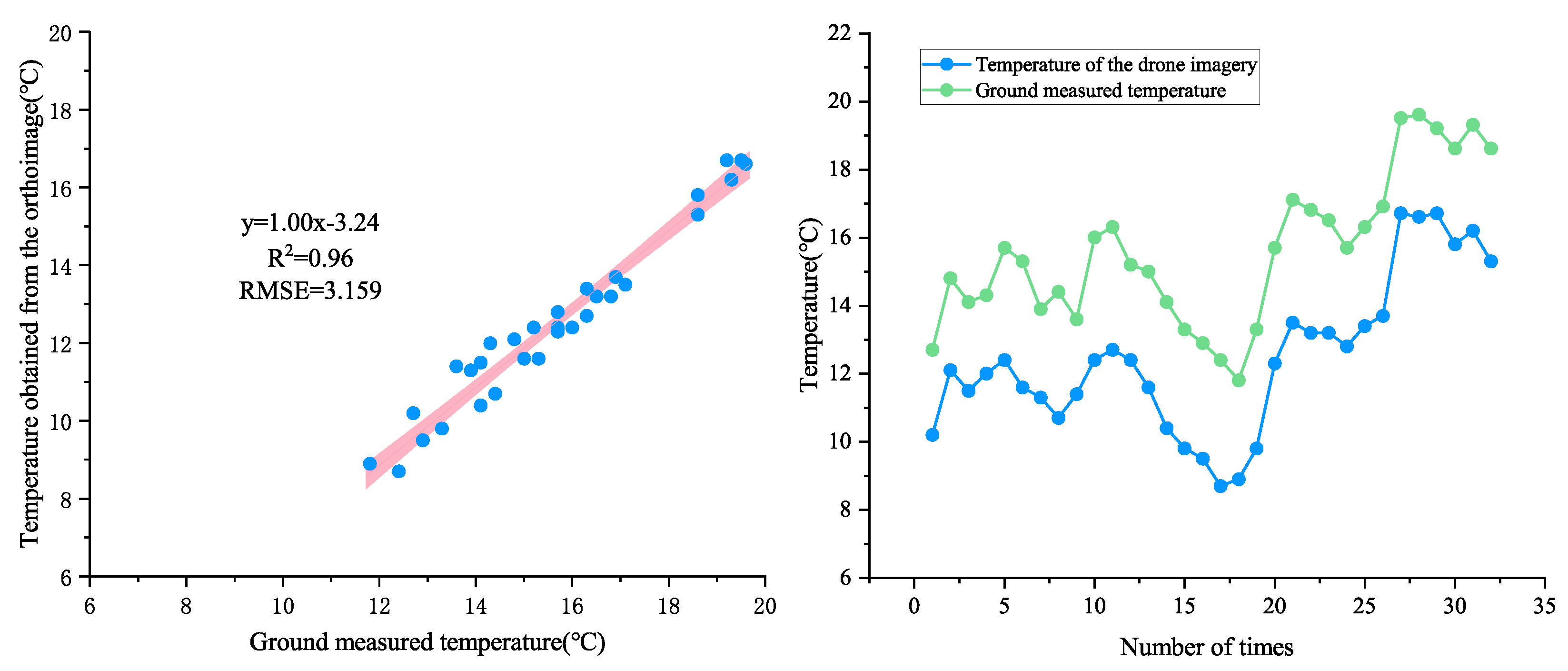
3.2. Unmanned Aerial Vehicle Thermal Infrared Image Temperature Correction

Figure 3 depicts the temperature measurements conducted during the cotton growth period using a handheld thermometer, in conjunction with water temperature data collected by the drone’s thermal infrared sensor at an operational altitude of 50 m. As an example, on 14 July 2022, the orthoimage temperature recorded by the drone was 12.4 °C, whereas the reference temperature was 15.2 °C, leading to a discrepancy of 2.8 °C. Through linear regression analysis of the dataset, an observation can be made that there existed a strong correlation between the temperatures extracted by the drone’s thermal infrared sensor and those measured by the handheld thermometer, with a coefficient of determination ($R^2$) of 0.96 and a root mean square error (RMSE) of 3.159 °C. The temperature correction process involved integrating and comparing temperature data obtained from the handheld thermometer and the drone’s thermal infrared sensor. Such an approach enabled a more precise acquisition of temperature information within the thermal infrared images captured by the drone. As such, the temperature correction improved the accuracy and reliability of subsequent analyses and research conducted using these images. This correction process can serve as a robust foundation for further analysis and research endeavours.

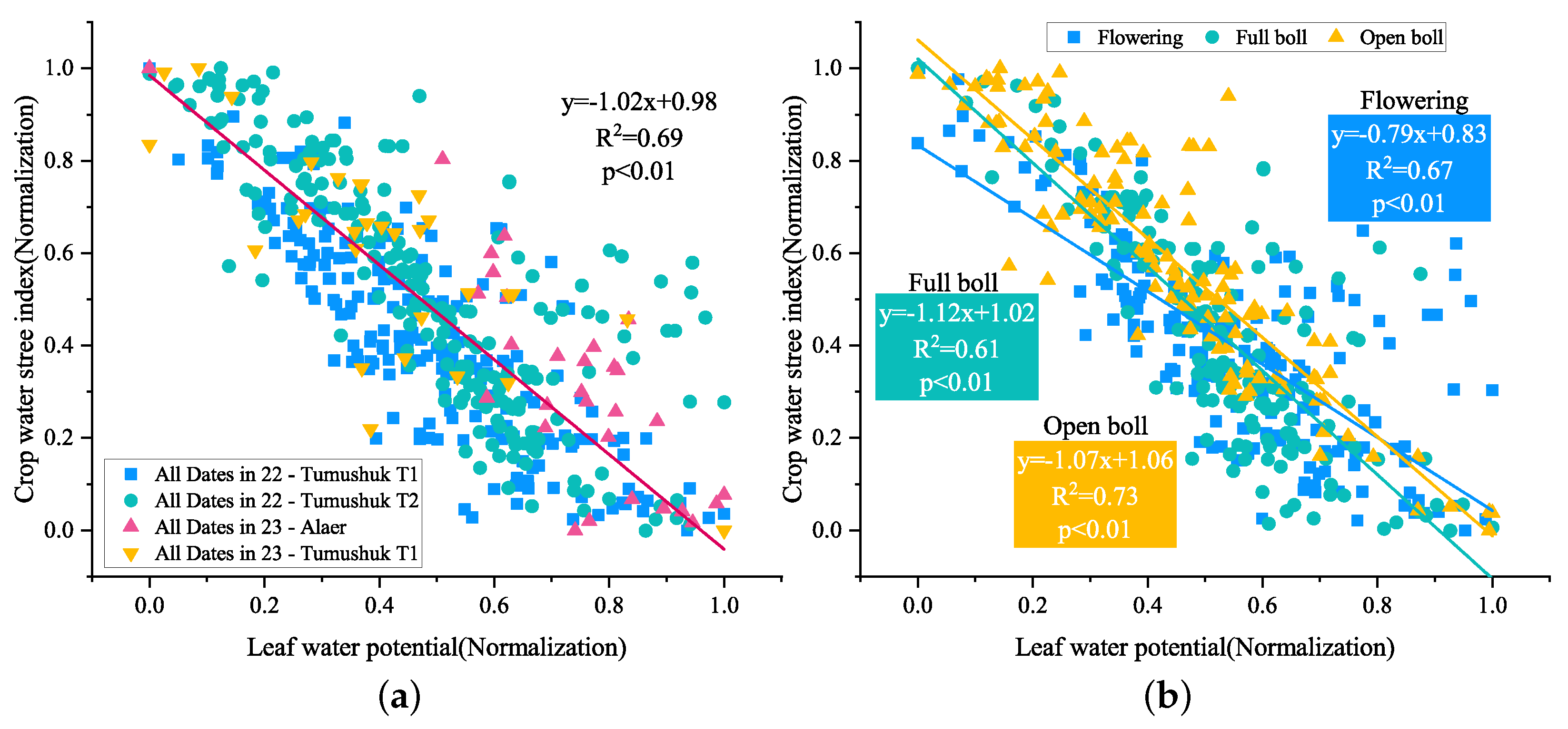
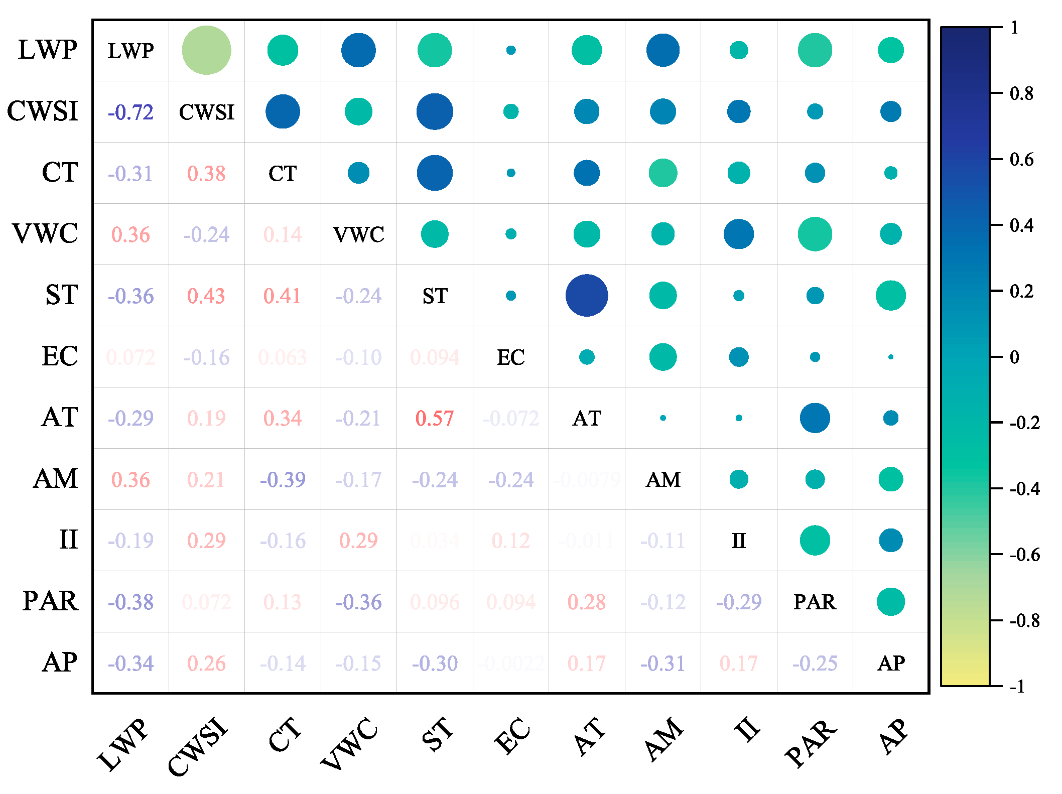
3.3. Relationship between the CWSI and LWP

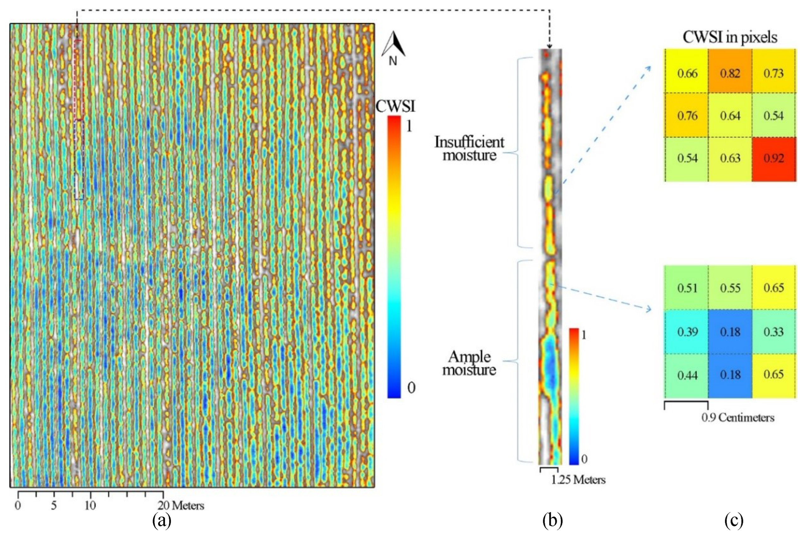
Linear regression analysis was conducted on the data collected during the 2022 and 2023 experiments to examine the relationship between the CWSI and LWP. As depicted in Figure 4, a strong linear relationship was observed between the CWSI and LWP ($R^2$ = 0.69). The model parameters (slope and intercept) exhibited significant differences in overall fit (p < 0.01). Across the three growth stages of cotton (flowering, full boll, and open boll), the linear relationship between the CWSI and LWP remained relatively stable. The coefficients of determination ($R^2$) for these stages were 0.67, 0.61, and 0.73, respectively. The model parameters (slope and intercept) also exhibited significant differences in overall fit (p < 0.01). These findings demonstrate the consistent linear relationship between the CWSI and LWP throughout the various growth stages of cotton, highlighting the potential for using the LWP as an indicator of a plant’s water status.

As shown in Figure 5, compared with the CWSI, the leaf water potential generally exhibited stronger correlations with various factors. Such findings indicate a closer association between the leaf water potential and the cotton plant’s water stress. Through comprehensive analysis, the leaf water potential can evidently serve as a direct indicator of plant water deficiency and plays a crucial role in assessing cotton plant water stress. Although the CWSI and soil volumetric water content can also provide insights into cotton plant water stress, they are more susceptible to influences from factors such as soil type, rainfall, and atmospheric temperature, which can potentially lead to inaccuracies in assessments. Therefore, when choosing water stress indicators, preference should be given to the leaf water potential indicator. However, measuring the leaf water potential notably requires specialised instruments and techniques, and the process can be intricate, making it less practical for large-scale applications. Thus, in practical field monitoring, a combination of other water stress indicators, such as the CWSI and soil volumetric water content, should be employed to provide a comprehensive assessment, thereby enhancing the accuracy of water stress monitoring.

3.4. CWSI Mapping

High-resolution images captured by the drone hold significant practical value in diagnosing cotton water stress conditions and can be used to generate maps of water stress distribution through simplified CWSI calculations. Figure 6a illustrates the adaptive estimated CWSI map based on T_wet and T_dry, demonstrating the variation in water status across the cotton field. The map demonstrates notable shifts in crop water stress within the experimental area. After the simplification process, the CWSI values for cotton plants ranged between 0 and 1, which closely aligns with the actual moisture content of cotton plants under various irrigation management practices across different plots. Figure 6b provides a detailed depiction of the areas within the cotton field experiencing water deficits and areas with a sufficient water supply. Figure 6c provides an enlarged view of the magnified CWSI pixel values (0.9 cm GSD).

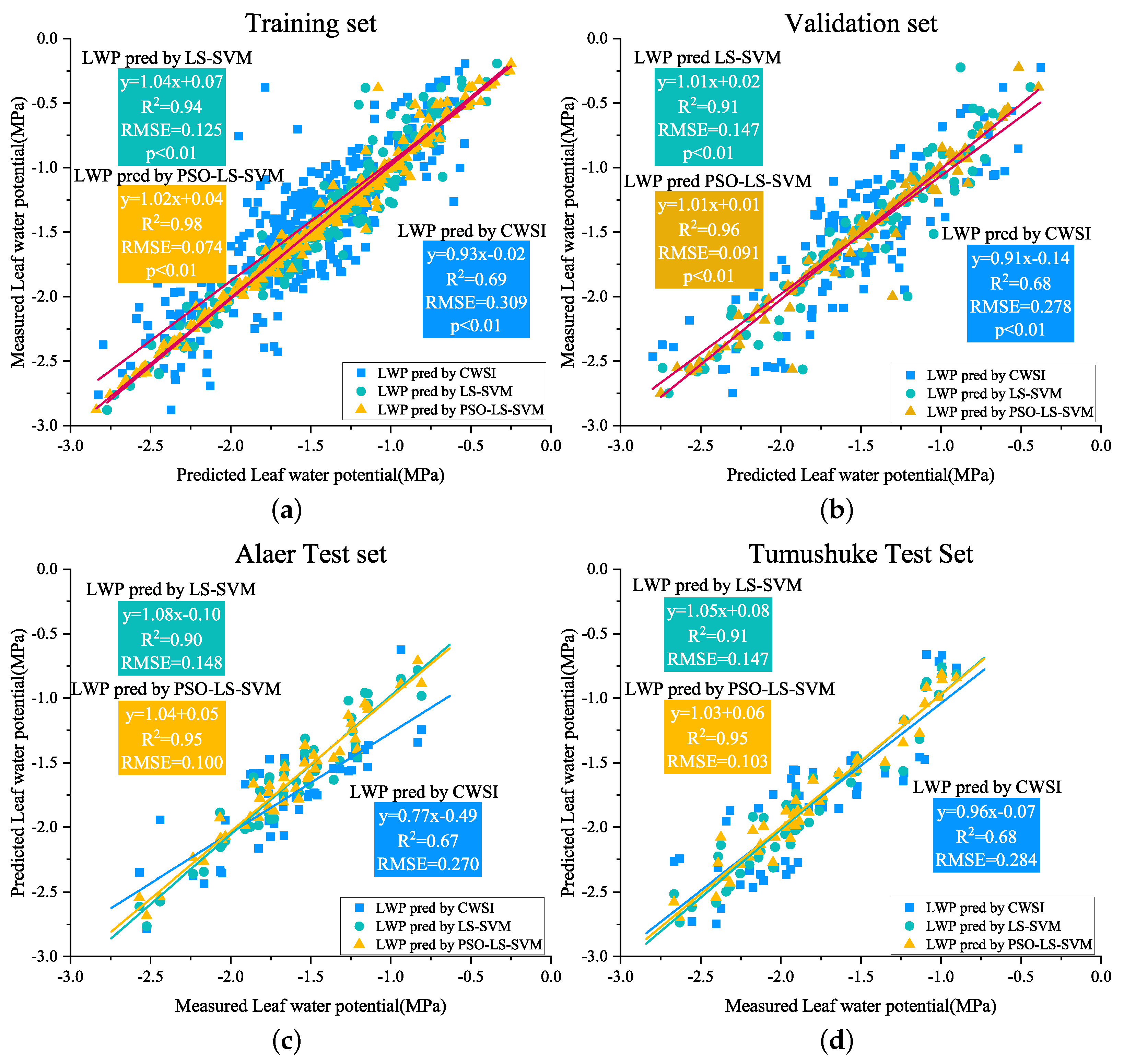
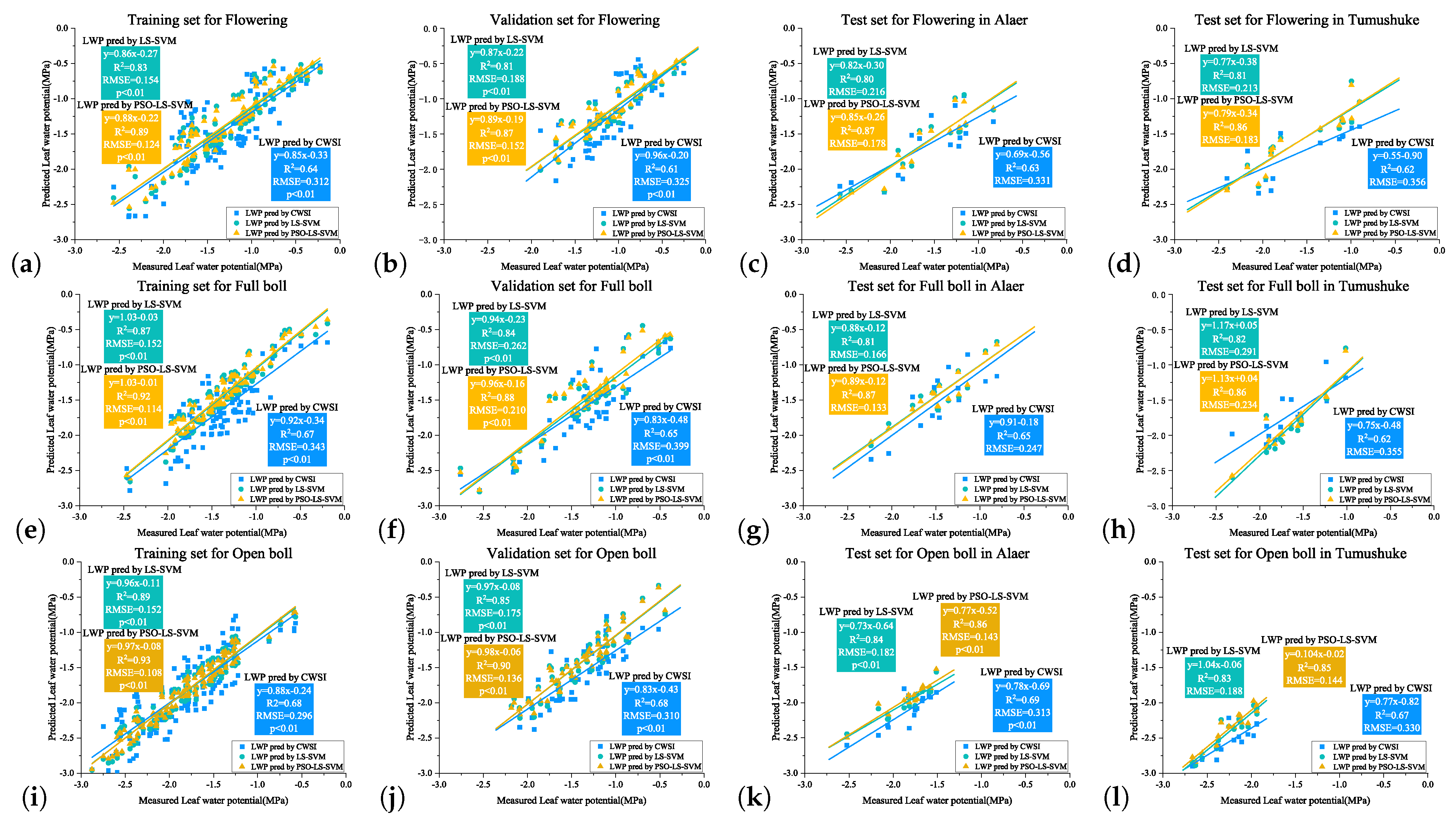
3.5. Performance Evaluation of the Leaf Water Potential Prediction Results

As depicted in Figure 7, predicting the leaf water potential using the CWSI is a frequently employed and straightforward method, but it tends to have relatively low accuracy and is susceptible to outlier values influenced by environmental factors. In contrast, the PSO-LS-SVM model exhibited significantly superior predictive accuracy and a lower error rate compared with both the CWSI and LS-SVM models. It particularly excelled in predicting the cotton leaf water potential. The PSO-LS-SVM model demonstrated a significant improvement in predictive accuracy, highlighting its ability to efficiently optimise model parameters and greatly enhance the performance of the traditional LS-SVM model.

When comparing the results related to errors in

Table 2. Comparison of model errors.

Model	Training Set		Validation Set		Alaer Test Set		Tumushuke Test Set
	RMSE	R2	RMSE	R2	RMSE	R2	RMSE	R2
CWSI	0.3093	0.6901	0.2780	0.6817	0.2709	0.6784	0.2845	0.6841
LS-SVM	0.1259	0.9487	0.1472	0.9145	0.1488	0.9003	0.1479	0.9137
PSO-LS-SVM	0.0742	0.9826	0.0916	0.9668	0.1002	0.9536	0.1033	0.9552

, the leaf water potential prediction model established through the PSO-LS-SVM method outperformed the model established through the LS-SVM method. Figure 7a presents the predictive outcomes of the training set. The model evidently exhibited a high correlation between the predicted and observed values on the training set, with an $R^2$ value of 0.98, signifying a favourable fit to the training data. Additionally, the RMSE was only 0.074, further confirming the model’s predictive accuracy. In Figure 7b, the model’s predictive performance on the validation set is displayed. Although there was a minor decline in the $R^2$ value when compared with the training set, the $R^2$ value still stood at 0.96, showcasing the strong generalisation capacity of the model. The RMSE on the validation set was 0.091, affirming the model’s predictive capability. Figure 7c illustrates the model’s predictive results on the Alaer test set. This test set presents challenges due to its diverse data sources from different years and regions. Nonetheless, the model achieved satisfactory outcomes, with an $R^2$ of 0.95 and an RMSE of 0.100, indicating strong predictive ability in the face of diverse data. Figure 7d demonstrates the model’s performance on datasets from the same region but different years. Similar to previous results, the model achieved a substantial $R^2$ value (0.95) and a relatively low RMSE value (0.103) on this dataset, confirming the model’s robustness across various data contexts.

The cotton leaf water potential soft measurement model established using the PSO-LS-SVM approach demonstrated higher accuracy and better predictive performance compared with the models built using the standard LS-SVM method. Furthermore, employing this approach for the prediction of the crop leaf water potential resulted in a greater estimation accuracy compared with both the statistical regression [25] and quantitative remote sensing [26] approaches. The predictive model founded on the PSO-LS-SVM approach effectively addresses the challenges associated with forecasting nonlinear agricultural data characterised by large volumes and high fluctuations.

After redividing the dataset, the predictive model was retrained with the aim of identifying the relationship between the cotton growth stages and leaf water potential from the flowering, full boll, and open boll data of 2022. The same model architecture as before was employed, and similar hyperparameter settings were maintained during the training process. Through the iterative optimisation process, the model gradually adapted to the data distribution. After the model training was concluded, it was subsequently applied to the datasets from 2023, which included the flowering, full boll, and open boll stages. This application aimed to evaluate the model’s predictive capacity in this new environmental context. The primary objective of this step was to ascertain whether the model could demonstrate generalisability across different years of data and generate accurate predictions for cotton leaf water potential.

Through the comparison results presented in

Table 3. Comparison of model errors.

Model	Flowering Test (Alaer)		Flowering Test (Tumushuke)		Full Boll Test (Alaer)		Full Boll Test (Tumushuke)		Open Boll Test (Alaer)		Open Boll Test (Tumushuke)
	RMSE	R2	RMSE	R2	RMSE	R2	RMSE	R2	RMSE	R2	RMSE	R2
CWSI	0.3318	0.6361	0.3563	0.6251	0.2475	0.6534	0.3551	0.6261	0.3136	0.6913	0.3304	0.6749
LS-SVM	0.2164	0.8089	0.2133	0.8174	0.1668	0.8137	0.2914	0.8260	0.1825	0.8436	0.1885	0.8343
PSO-LS-SVM	0.1784	0.8712	0.1836	0.8643	0.1336	0.8746	0.2347	0.8672	0.1436	0.8632	0.1440	0.8559

, an observation can be made that the model continued to exhibit relatively accurate predictive performance on the new datasets. In Figure 8a,e,i, the PSO-LS-SVM model achieved $R^2$ values of 0.89, 0.92, and 0.93 for the training set during the flowering, full boll, and open boll stages with RMSE values of 0.124, 0.114, and 0.108, respectively. In Figure 8b,f,j, the PSO-LS-SVM model attained $R^2$ values of 0.87, 0.88, and 0.90 for the validation set during the flowering, full boll, and open boll stages with RMSE values of 0.152, 0.210, and 0.136, respectively. Figure 8c,d displays the testing results for the flowering stage data in the work of Alaer and Tumushuke in 2023, with $R^2$ values of 0.87 and 0.86 and RMSE values of 0.178 and 0.183, respectively. Figure 8g,h depicts the testing results for the full boll data in the work of Alaer and Tumushuke in 2023, with $R^2$ values of 0.87 and 0.86 and RMSE values of 0.133 and 0.234, respectively. Finally, Figure 8k,l exhibits the testing results for the open boll data in the work of Alaer and Tumushuke in 2023, with $R^2$ values of 0.86 and 0.85 and RMSE values of 0.143 and 0.144, respectively. Such findings further substantiate the robustness and generalisation capacity of the predictive model for the leaf water potential across diverse geographical contexts. Nevertheless, when juxtaposed with the model’s performance on the comprehensive growth period dataset, noticeable instances of reduced accuracy become evident. This decline in accuracy may be attributed to the constraint of having a diminished number of training samples. The dataset was partitioned again, resulting in a reduced quantity of samples available for training and potentially constraining the model’s ability to capture the global data distribution. In situations characterised by limited data points, it becomes imperative to exercise prudence when interpreting and evaluating the model’s performance. In practical applications, the prospect of enhancing the model’s performance with a reduced training dataset lies in the pursuit of additional data collection and optimisation efforts.

4. Discussion

Thermal infrared imagery serves as an effective means to expand ground-based measurements for assessing the spatial distribution of the crop water status at the field scale. Nonetheless, the precise identification of vegetation canopy pixels and the acquisition of temperature values that accurately represent the vegetation’s thermal characteristics without interference from the soil background present challenges. In the present study, the Canny edge detection algorithm was deployed to mitigate the presence of ambiguous mixed pixels. Additionally, critical thresholds for the CWSI were established by considering the temperature distribution in the thermal infrared imagery, specifically targeting the 0.5% and 99.5% temperature percentiles. These thresholds were instrumental in defining T_wet and T_dry. Utilizing a single reference temperature value to characterise the entire study area would lead to biased and non-representative CWSI results, especially in fields composed of different crop varieties or canopy structures. Even under the same irrigation regime, varying water use efficiency for individual crops due to factors such as soil characteristics, terrain elevation, and uneven irrigation management can result in temperature variations. Consequently, the accuracy of CWSI-based evaluations of the cotton water status can be compromised.

The LWP has been widely accepted as an indicator of crop water status [27]. As such, many crop growers and physiological researchers have employed pressure chamber methods to determine the water status of crops, particularly for vegetables and grapes [28,29]. In the context of cotton plants, a strong correlation exists between the leaf water potential and water stress. When cotton plants undergo water stress, they encounter difficulty in extracting an adequate amount of water from the soil. This leads to a decrease in the water content within the leaves, consequently causing a reduction in the leaf water potential. The decline in the leaf water potential gives rise to observable effects such as leaf wilting, loss of pigmentation, and tissue necrosis. These physiological changes ultimately have a detrimental impact on the growth and development of cotton plants. Therefore, the leaf water potential is a crucial indicator for assessing the degree of water stress in cotton. When the leaf water potential decreases to a certain level, timely irrigation is needed to maintain normal plant growth, enhance cotton yields, and improve quality.

However, while assessing the crop water status through the LWP is a reliable method, practical limitations emerge when attempting to apply it at the field scale, primarily due to constraints related to resources such as labour and equipment. This leads to a restricted spatial coverage. Machine learning algorithms can be utilised for LWP prediction, enabling the mapping of the cotton water status to cover large areas. The LWP map in Figure 9 was created using the PSO-LS-SVM model. This map displays the spatial variation in the LWP predicted by the model using multiple data sources. In the domain of digital agriculture, the utilisation of thermal infrared remote sensing conducted via UAVs presents significant promise, but it is not without its set of challenges [30,31]. After analysing the cotton canopy images obtained through UAV thermal infrared remote sensing, significant differences in canopy temperature were found [32,33,34]. Therefore, accurate prediction of cotton’s leaf water potential is crucial for assessing water stress and enhancing cotton quality. In recent years, the combined PSO and LS-SVM model has been widely applied for crop growth monitoring and predicting related data [35,36,37]. In future research endeavours, the exploration of supplementary feature extraction techniques for multi-source data has the potential to enhance the performance of models. At the same time, the integration of alternative optimisation algorithms and machine learning methods holds promise for the development of more intricate and precise prediction models. Additionally, this method is applicable to predicting the leaf water potential in other crops. This comprehensive data analysis approach holds the promise of conducting comprehensive assessments of growth and moisture conditions in various crops, contributing to the management of irrigation processes and the evaluation of plant health in other agricultural and orchard plants. In the future, the integration of spectral indices (such as the NDVI or NDWI) from multispectral remote sensing data, temperature information from thermal infrared imaging data, and texture information will enable a more comprehensive assessment of crop health and moisture conditions.

5. Conclusions

In the present study, a machine learning algorithm based on multi-source data was utilised to establish a predictive model using a combination of UAV remote sensing imagery, meteorological, and soil data. The model was constructed based on the LS-SVM approach and subsequently fine-tuned using the PSO algorithm to forecast cotton’s leaf water potential and generate distribution maps. The outcomes highlight that, in comparison with conventional linear regression models employing the CWSI, the LS-SVM model notably enhanced the prediction accuracy. On two test sets, the $R^2$ values reached 0.90 and 0.91, with corresponding RMSE values of 0.148 and 0.147. After PSO optimisation, the $R^2$ value increased by 0.05 and 0.04, with both achieving a result of 0.95, and the RMSE reduced to 0.100 and 0.103, respectively. Such results indicate that the model performed well in predicting cotton’s leaf water potential and shows promise as a potential model for such predictions.

The model was trained using data from the 2022 flowering, full boll, and open boll stages of cotton. Evaluations were then conducted using test sets for the flowering, full boll, and open boll stages of cotton in the cities of Alaer and Tumushuke in 2023. The results show that the model also performed with relatively high accuracy on these new test sets. For the flowering stage test set, the $R^2$ values were 0.87 and 0.86, with corresponding RMSE values of 0.178 and 0.183. In the full boll stage test set, the $R^2$ values were 0.87 and 0.86, with corresponding RMSE values of 0.133 and 0.234. For the open boll stage test set, the $R^2$ values were 0.86 and 0.85, with corresponding RMSE values of 0.143 and 0.144. Such findings further confirm the robustness and generalisation ability of the leaf water potential prediction model, as well as its adaptability to different geographical environments. This development opens up new avenues for precision agriculture management, offering valuable insights to decision makers seeking a more comprehensive understanding of plant growth conditions.

References

1. Zhou, Z.; Majeed, Y.; Naranjo, G.D.; Gambacorta, E.M.T. Assessment for crop water stress with infrared thermal imagery in precision agriculture: A review and future prospects for deep learning applications. Comput. Electron. Agric. 2021, 182, 106019. [Google Scholar] [CrossRef]
2. Chandel, A.K.; Khot, L.R.; Yu, L.X. Alfalfa (Medicago sativa L.) crop vigor and yield characterization using high-resolution aerial multispectral and thermal infrared imaging technique. Comput. Electron. Agric. 2021, 182, 105999. [Google Scholar] [CrossRef]
3. Carrasco-Benavides, M.; Viejo, C.G.; Tongson, E.; Baffico-Hern’andez, A.; ’Avila-S’anchez, C.; Mora, M.; Fuentes, S. Water status estimation of cherry trees using infrared thermal imagery coupled with supervised machine learning modeling. Comput. Electron. Agric. 2022, 200, 107256. [Google Scholar] [CrossRef]
4. Cohen, Y.; Alchanatis, V.; Meron, M.; Saranga, Y.; Tsipris, J. Estimation of leaf water potential by thermal imagery and spatial analysis. J. Exp. Bot. 2005, 56, 1843–1852. [Google Scholar] [CrossRef] [PubMed]
5. Alchanatis, V.; Cohen, Y.; Cohen, S.; Moller, M.; Sprinstin, M.; Meron, M.; Tsipris, J.; Saranga, Y.; Sela, E. Evaluation of different approaches for estimating and mapping crop water status in cotton with thermal imaging. Precis. Agric. 2010, 11, 27–41. [Google Scholar] [CrossRef]
6. Berni, J.A.J.; Zarco-Tejada, P.J.; Sepulcre-Cant’o, G.; Fereres, E.; Villalobos, F. Mapping canopy conductance and CWSI in olive orchards using high resolution thermal remote sensing imagery. Remote. Sens. Environ. 2009, 113, 2380–2388. [Google Scholar] [CrossRef]
7. Gonzalez-Dugo, V.; Zarco-Tejada, P.; Berni, J.A.J.; Suarez, L.; Goldhamer, D.; Fereres, E. Almond tree canopy temperature reveals intra-crown variability that is water stress-dependent. Agric. For. Meteorol. 2012, 154, 156–165. [Google Scholar] [CrossRef]
8. Gonzalez-Dugo, V.; Zarco-Tejada, P.; Nicol’as, E.; Nortes, P.A.; Alarc’on, J.J.; Intrigliolo, D.S.; Fereres, E. Using high resolution UAV thermal imagery to assess the variability in the water status of five fruit tree species within a commercial orchard. Precis. Agric. 2013, 14, 660–678. [Google Scholar] [CrossRef]
9. Meron, M.; Tsipris, J.; Orlov, V.; Alchanatis, V.; Cohen, Y. Crop water stress mapping for site-specific irrigation by thermal imagery and artificial reference surfaces. Precis. Agric. 2010, 11, 148–162. [Google Scholar] [CrossRef]
10. O’shaughnessy, S.A.; Evett, S.R.; Colaizzi, P.D.; Howell, T.A. Using radiation thermography and thermometry to evaluate crop water stress in soybean and cotton. Agric. Water Manag. 2011, 98, 1523–1535. [Google Scholar] [CrossRef]
11. Kirnak, H.; Irik, H.; Unlukara, A. Potential use of crop water stress index (CWSI) in irrigation scheduling of drip-irrigated seed pumpkin plants with different irrigation levels. Sci. Hortic. 2019, 256, 108608. [Google Scholar] [CrossRef]
12. Cohen, Y.; Alchanatis, V.; Saranga, Y.; Rosenberg, O.; Sela, E.; Bosak, A.J. Mapping water status based on aerial thermal imagery: Comparison of methodologies for upscaling from a single leaf to commercial fields. Precis. Agric. 2017, 18, 801–822. [Google Scholar] [CrossRef]
13. Browne, M.; Yardimci, N.T.; Scoffoni, C.; Jarrahi, M.; Sack, L. Prediction of leaf water potential and relative water content using terahertz radiation spectroscopy. Plant Direct 2020, 4, e00197. [Google Scholar] [CrossRef] [PubMed]
14. Fulton, A.; Grant, J.; Buchner, R.; Connell, J. Using the Pressure Chamber for Irrigation Management in Walnut, Almond and Prune. 2014. Available online: https://escholarship.org/uc/item/2m2719gm (accessed on 9 November 2023).
15. Meron, M.; Sprintsin, M.; Tsipris, J.; Alchanatis, V.; Cohen, Y. Foliage temperature extraction from thermal imagery for crop water stress determination. Precis. Agric. 2013, 14, 467–477. [Google Scholar] [CrossRef]
16. Sagan, V.; Maimaitijiang, M.; Sidike, P.; Eblimit, K.; Peterson, K.T.; Hartling, S.; Esposito, F.; Khanal, K.; Newcomb, M.; Pauli, D.; et al. UAV-based high resolution thermal imaging for vegetation monitoring, and plant phenotyping using ICI 8640 P, FLIR Vue Pro R 640, and thermomap cameras. Remote. Sens. 2019, 11, 330. [Google Scholar] [CrossRef]
17. Bian, J.; Zhang, Z.; Chen, J.; Chen, H.; Cui, C.; Li, X.; Chen, S.; Fu, Q. Simplified evaluation of cotton water stress using high resolution unmanned aerial vehicle thermal imagery. Remote. Sens. 2019, 11, 267. [Google Scholar] [CrossRef]
18. Youssef Ali Amer, A. Global-local least-squares support vector machine (GLocal-LS-SVM). PLoS ONE 2023, 18, e0285131. [Google Scholar] [CrossRef]
19. Wang, H.; Hu, D. Comparison of SVM and LS-SVM for regression. In Proceedings of the IEEE 2005 International Conference on Neural Networks and Brain, Beijing, China, 13–15 October 2005; Volume 1, pp. 279–283. [Google Scholar]
20. Ahmad, M.W.; Reynolds, J.; Rezgui, Y. Predictive modelling for solar thermal energy systems: A comparison of support vector regression, random forest, extra trees and regression trees. J. Clean. Prod. 2018, 203, 810–821. [Google Scholar] [CrossRef]
21. Hittawe, M.M.; Sidibé, D.; Mériaudeau, F. Bag of words representation and SVM classifier for timber knots detection on color images. In Proceedings of the IEEE 2015 14th IAPR International Conference on Machine Vision Applications (MVA), Tokyo, Japan, 18–22 May 2015; pp. 287–290. [Google Scholar]
22. Bouindour, S.; Hittawe, M.M.; Mahfouz, S.; Snoussi, H. Abnormal event detection using convolutional neural networks and 1-class SVM classifier. In Proceedings of the 8th International Conference on Imaging for Crime Detection and Prevention (ICDP 2017), Madrid, Spain, 13–15 December 2017; pp. 1–6. [Google Scholar]
23. Zhou, C.; Ding, L.; Zhou, Y.; Zhang, H.; Skibniewski, M.J. Hybrid support vector machine optimization model for prediction of energy consumption of cutter head drives in shield tunneling. J. Comput. Civ. Eng. 2019, 33, 04019019. [Google Scholar] [CrossRef]
24. Lacerda, L.N.; Snider, J.L.; Cohen, Y.; Liakos, V.; Gobbo, S.; Vellidis, G. Using UAV-based thermal imagery to detect crop water status variability in cotton. Smart Agric. Technol. 2022, 2, 100029. [Google Scholar] [CrossRef]
25. Cowan, I.R. Transport of water in the soil-plant-atmosphere system. J. Appl. Ecol. 1965, 2, 221–239. [Google Scholar] [CrossRef]
26. Liu, N.; Deng, Z.; Wang, H.; Luo, Z.; Guti’errez-Jurado, H.A.; He, X.; Guan, H. Thermal remote sensing of plant water stress in natural ecosystems. For. Ecol. Manag. 2020, 476, 118433. [Google Scholar] [CrossRef]
27. Scholander, P.F.; Bradstreet, E.D.; Hemmingsen, E.A.; Hammel, H.T. Sap Pressure in Vascular Plants: Negative hydrostatic pressure can be measured in plants. Science 1965, 148, 339–346. [Google Scholar] [CrossRef] [PubMed]
28. Parkash, V.; Singh, S. A review on potential plant-based water stress indicators for vegetable crops. Sustainability 2020, 12, 3945. [Google Scholar] [CrossRef]
29. Gambetta, G.A.; Herrera, J.C.; Dayer, S.; Feng, Q.; Hochberg, U.; Castellarin, S.D. The physiology of drought stress in grapevine: Towards an integrative definition of drought tolerance. J. Exp. Bot. 2020, 71, 4658–4676. [Google Scholar] [CrossRef]
30. Gago, J.; Douthe, C.; Coopman, R.E.; Gallego, P.P.; Ribas-Carbo, M.; Flexas, J.; Escalona, J.B.; Medrano, H. UAVs challenge to assess water stress for sustainable agriculture. Agric. Water Manag. 2015, 153, 9–19. [Google Scholar] [CrossRef]
31. Colomina, I.; Molina, P. Unmanned aerial systems for photogrammetry and remote sensing: A review. ISPRS J. Photogramm. Remote. Sens. 2014, 92, 79–97. [Google Scholar] [CrossRef]
32. Merlaud, A.; Tack, F.; Constantin, D.; Georgescu, L.; Maes, J.; Fayt, C.; Mingireanu, F.; Schuettemeyer, D.; Meier, A.C.; Sch"onardt, A.; et al. The Small Whiskbroom Imager for atmospheric composition monitoring (SWING) and its operations from an unmanned aerial vehicle (UAV) during the AROMAT campaign. Atmos. Meas. Tech. 2018, 11, 551–567. [Google Scholar] [CrossRef]
33. Biju, S.; Fuentes, S.; Gupta, D. The use of infrared thermal imaging as a non-destructive screening tool for identifying drought-tolerant lentil genotypes. Plant Physiol. Biochem. 2018, 127, 11–24. [Google Scholar] [CrossRef]
34. Li, W.; Liu, C.; Yang, Y.; Awais, M.; Li, W.; Ying, P.; Ru, W.; Cheema, M.J.M. A UAV-aided prediction system of soil moisture content relying on thermal infrared remote sensing. Int. J. Environ. Sci. Technol. 2022, 19, 9587–9600. [Google Scholar] [CrossRef]
35. Liu, X.S.; Sun, F.F.; Jin, Y.; Wu, Y.J.; Gu, Z.X.; Zhu, L.; Yan, D.L. Application of near infrared spectroscopy combined with particle swarm optimization based least square support vector machine to rapid quantitative analysis of Corni Fructus. Yao Xue Xue Bao Acta Pharm. Sin. 2015, 50, 1645–1651. [Google Scholar]
36. Zakeri, M.S.; Mousavi, S.F.; Farzin, S.; Sanikhani, H. Modeling of reference crop evapotranspiration in wet and dry climates using data-mining methods and empirical equations. J. Soft Comput. Civ. Eng. 2022, 6, 1–28. [Google Scholar]
37. Priyadharshini, K.; Prabavathi, R.; Devi, V.B.; Subha, P.; Saranya, S.M.; Kiruthika, K. An Enhanced Approach for Crop Yield Prediction System Using Linear Support Vector Machine Model. In Proceedings of the 2022 International Conference on Communication, Computing and Internet of Things (IC3IoT), IEEE, Chennai, India, 10–11 March 2022; pp. 1–5. [Google Scholar]
Figure 1. (a) Tumushuke test area. (b) Alaer test area.
Agronomy 13 02929 g001
Figure 2. (a) Original thermal infrared image. (b) Thermal infrared image after lens distortion correction. (c) Visible light image used for canopy extraction. (d) Thermal infrared-visible light aligned image for canopy extraction. (e) Temperature distribution map of the thermal infrared image. (f) Canopy mask of cotton after soil background removal using the Canny edge detection algorithm. (g) Temperature distribution histogram of the original thermal infrared image. (h) Temperature distribution histogram of the canopy after soil background removal.
Agronomy 13 02929 g002
Figure 3. Comparison between ground-measured temperature and drone orthophoto temperature.
Agronomy 13 02929 g003
Figure 4. (a) Inverse linear regression between CWSI and LWP for different times and regions (data normalised). (b) Inverse linear regression between CWSI and LWP during cotton flowering, full boll, and open boll stages (data normalised).
Agronomy 13 02929 g004
Figure 5. Correlation coefficients of water stress indicators. Compared with CWSI, leaf water potential (LWP) generally exhibited stronger correlations with various factors: canopy temperature (CT), volumetric water content (VWC), soil temperature (ST), electrical conductivity (EC), atmospheric temperature (AT), atmospheric moisture (AM), illumination intensity (II), photosynthetically active radiation (PAR), and atmospheric pressure (AP).
Agronomy 13 02929 g005
Figure 6. (a) CWSI map obtained through unmanned aerial vehicle remote sensing using thermal infrared imagery. (b) Example of a CWSI map depicting insufficient moisture and ample moisture areas of cotton. (c) Example of pixel-level resolution in the CWSI map.
Agronomy 13 02929 g006
Figure 7. Comparison of predicted LWP values with actual values using three different methods: CWSI, LS-SVM, and PSO-LS-SVM. (a) Training set. (b) Validation set. (c) Alaer test set. (d) Tumushuke test set.
Agronomy 13 02929 g007
Figure 8. Comparison of predicted LWP values with actual values for the newly partitioned dataset. (a) The 2022 Alaer flowering period training set. (b) The 2022 Alaer flowering period validation set. (c) The 2023 Alaer flowering period test set. (d) The 2023 Tumushuke flowering period test set. (e) The 2022 Alaer full boll period training set. (f) The 2022 Alaer full boll period validation set. (g) The 2023 Alaer full boll period test set. (h) The 2023 Tumushuke full boll period test set. (i) The 2022 Alaer open boll period training set. (j) The 2022 Alaer open boll period validation set. (k) The 2023 Alaer open boll period test set. (l) The 2023 Tumushuke open boll period test set.
Agronomy 13 02929 g008
Figure 9. Leaf water potential map.
Agronomy 13 02929 g009