Assessing the Relative Importance of Climatic and Hydrological Factors in Controlling Sap Flow Rates for a Riparian Mixed Stand


Abstract
:1. Introduction
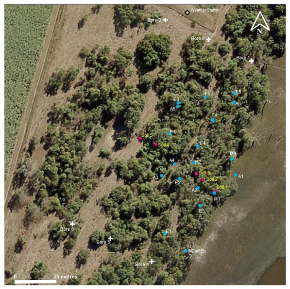
2. Site Description
2.1. Climate
2.2. Hydrology and Hydrogeology
2.3. Soils
2.4. Vegetation
3. Materials and Methods
3.1. Climate
3.2. Tree Selection
3.3. Tree Water Use
3.4. Soil Moisture
3.5. Tree Growth
3.6. Groundwater and Surface Water
3.7. Data Analyses
4. Results
4.1. Soil Water Trends
4.2. Groundwater Level Trends
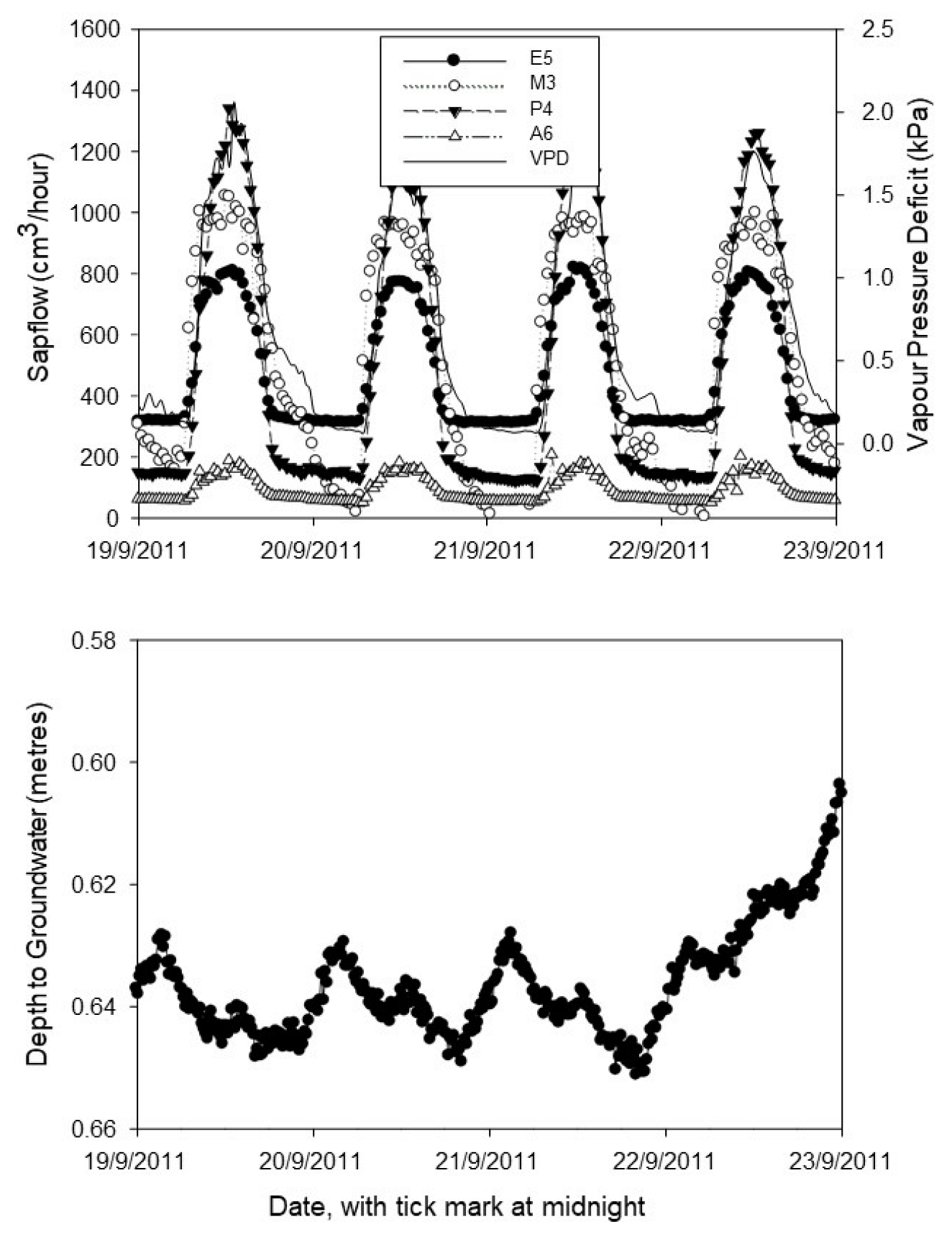
4.3. Sap flow Rates
4.4. Diurnal Trends and Nocturnal Sap flow
4.5. Sap flow Variations with Depth to Groundwater
4.6. Which Factors Are Most Important in Influencing Sap Flow?
5. Discussion
5.1. Evidence of Groundwater Dependence
5.2. Is Depth to Groundwater a Strong Predictor of Sap Flow Rates?
5.3. Is Distance to Surface Water a Strong Predictor of Sap Flow Rates?
5.4. Methods
6. Conclusions
Author Contributions
Funding
Data Availability Statement
Acknowledgments
Conflicts of Interest
References
- Baird, K.J.; Maddock, T.I. Simulating riparian evapotranspiration: A new methodology and application for groundwater models. J. Hydrol. 2005, 312, 176–190. [Google Scholar] [CrossRef]
- Satchithanantham, S.; Wilson, H.F.; Glenn, A.J. Contrasting patterns of groundwater evapotranspiration in grass and tree dominated riparian zones of a temperate agricultural catchment. J. Hydrol. 2017, 549, 654–666. [Google Scholar] [CrossRef]
- Orellana, F.; Verma, P.; Loheide, S.P.; Daly, E. Monitoring and modeling water-vegetation interactions in groundwater-dependent ecosystems. Rev. Geophys. 2012, 50. [Google Scholar] [CrossRef]
- Evans, R. The Impact of Groundwater Use on Australia’s Rivers: Technical Report; Land and Water Australia: Canberra, Australia, 2007. [Google Scholar]
- Loheide, S.P.; Butler, J.J.; Gorelick, S.M. Use of diurnal water table fluctuations to estimate groundwater consumption by phreatophytes: A saturated-unsaturated flow assessment. Water Resour. Res. 2005, 41, W07030. [Google Scholar] [CrossRef]
- White, W.N. A Method for Estimating Ground-Water Supplies Based on Discharge by Plants and Evaporation from soil—Results of Investigations in Escalante Valley, Utah; US Government Printing Office: Washington, DC, USA, 1932; Volume 105. [Google Scholar]
- Butler, J.J.; Kluitenberg, G.J.; Whittemore, D.O.; Loheide, S.P.; Jin, W.; Billinger, A.; Zhan, X. A field investigation of phreatophyte-induced fluctuations in the water table. Water Resour. Res. 2007, 43. [Google Scholar] [CrossRef] [Green Version]
- Forster, M.A. How significant is nocturnal sap flow? Tree Physiol. 2014, 34, 757–765. [Google Scholar] [CrossRef] [Green Version]
- Zeppel, M.J.B.; Lewis, J.D.; Phillips, N.G.; Tissue, D.T. Consequences of nocturnal water loss: A synthesis of regulating factors and implications for capacitance, embolism and use in models. Tree Physiol. 2014, 34, 1047–1055. [Google Scholar] [CrossRef] [Green Version]
- Fan, J.; Ostergaard, K.T.; Guyot, A.; Fujiwara, S.; Lockington, D.A. Estimating groundwater evapotranspiration by a subtropical pine plantation using diurnal water table fluctuations: Implications for night-time water use. J. Hydrol. 2016, 542, 679–685. [Google Scholar] [CrossRef] [Green Version]
- Larsen, E.K.; Palau, J.L.; Valiente, J.A.; Chirino, E.; Bellot, J. Technical note: Long-term probe misalignment and proposed quality control using the heat pulse method for transipration estimations. Hydrol. Earth Syst. Sci. 2020, 24, 2755–2767. [Google Scholar] [CrossRef]
- Steinberg, S.L.; McFarland, M.J.; Worthington, J.W. A gauge to measure mass flow rate of sap in stems and trunks of woody plants. J. Am. Soc. Hortic. Sci. 1989, 114, 466–472. [Google Scholar] [CrossRef]
- Eamus, D.; Zolfaghar, S.; Villalobos-Vega, R.; Cleverly, J.; Huete, A. Groundwater-dependent ecosystems: Recent insights from satellite and field-based studies. Hydrol. Earth Syst. Sci. 2015, 19, 4229–4256. [Google Scholar] [CrossRef] [Green Version]
- O’Grady, A.; Eamus, D.; Cook, P.G.; Lamontagne, S. Groundwater use by riparian vegetation in the we-dry tropics of northern Australia. Aust. J. Bot. 2006, 54, 145–154. [Google Scholar] [CrossRef]
- Holsher, D.; Kock, O.; Korn, S.; Leuschner, C. Sap flux of five co-occuring tree species in a temperate broad-leaved forest during seasonal soil drought. Trees 2005, 19, 628–637. [Google Scholar] [CrossRef]
- Doble, R.C.; Crosbie, R.S. Review: Current and emerging methods for catchment-scale modelling of rechare and evapotranspiration from shallow groundwater. Hydrogeol. J. 2017, 25, 3–23. [Google Scholar] [CrossRef]
- Huang, Y.Q.; Li, X.K.; Zhang, Z.F.; He, C.X.; Zhao, P.; You, Y.M.; Mo, L. Seasonal changes in Cyclobalanopsis glauca transpiration and canopy stomatal conductance and their dependence on subterranean water and climatic factors in rocky karst terrain. J. Hydrol. 2011, 402, 135–143. [Google Scholar] [CrossRef]
- Yunusa, I.A.M.; Nuberg, I.K.; Fuentes, S.; Lu, P.; Eamus, D. A simple field validation of daily transpiration derived from sapflow using a porometer and minimal meteorological data. Plant Soil 2008, 305, 15–24. [Google Scholar] [CrossRef]
- Johnson, B.; Malama, B.; Barrash, W.; Flores, A.N. Recognizing and modeling variable drawdown due to evapotranspiration in a semiaride riparian zone considering local differences in vegetation and distance from a river source. Water Resour. Res. 2013, 49, 1030–1039. [Google Scholar] [CrossRef] [Green Version]
- Benyon, R.G. Nighttime water use in an irrigated Eucalyptus grandis plantation. Tree Physiol. 1999, 19, 853–859. [Google Scholar] [CrossRef]
- Hatton, T.J.; Moore, S.J.; Reece, P.H. Estimating stand transpiration in a Eucalyptus populnea woodland with the heat pulse method: Measurement errors and sampling strategies. Tree Physiol. 1995, 15, 219–227. [Google Scholar] [CrossRef]
- McJannet, D. Water table and transpiration dynamics in a seasonally inundated Melaleuca quinquenervia forest, north Queensland, Australia. Hydrol. Process. 2008, 22, 3079–3090. [Google Scholar] [CrossRef]
- O’Grady, A.; Eamus, D.; Cook, P.G.; Lamontagne, S. Comparative water use by the riparian trees Melaleuca argentea and Corymbia bella in the wet-dry tropics of northern Australia. Aust. J. Bot. 2005, 54, 145–154. [Google Scholar] [CrossRef]
- Madurapperuma, W.S.; Bleby, T.M.; Burgess, S.S.O. Evaluation of sap flow methods to determine water use by cultivated palms. Environ. Exp. Bot. 2009, 66, 372–380. [Google Scholar] [CrossRef]
- ANCA (Australian Nature Conservation Agency). A Directory of Important Wetlands in Australia, 2nd ed.; Australian Nature Conservation Agency: Canberra, Australia, 1996. [Google Scholar]
- Burgess, S.S.O.; Adams, M.A.; Turner, N.C.; Beverly, C.R.; Ong, C.K.; Khan, A.A.H.; Bleby, T.M. An improved heat pulse method to measure low and reverse rates of sap flow in woody plants. Tree Physiol. 2001, 21, 589–598. [Google Scholar] [CrossRef] [PubMed]
- Edwards, W.R.N.; Becker, P.; Cermak, J. A unified nomenclature for sap flow measurements. Tree Physiol. 1996, 17, 65–67. [Google Scholar] [CrossRef] [Green Version]
- Marshall, D.C. Measurement of sap flow in conifers by heat transport. Plant Physiol. 1958, 33, 385–396. [Google Scholar] [CrossRef] [PubMed] [Green Version]
- Barrett, D.J.; Hatton, T.J.; Ash, J.E.; Ball, M.C. Evaluation of the heat pulse velocity technique for measurement of sap flow in rainforest and eucalypt forest species of south-eastern Australia. Plant Cell Environ. 1995, 18, 463–469. [Google Scholar] [CrossRef]
- Becker, P.; Edwards, W.R.N. Corrected heat capacity of wood for sap flow calculations. Tree Physiol. 1999, 19, 767–768. [Google Scholar] [CrossRef] [Green Version]
- Gwenzi, W.; Veneklaas, E.J.; Bleby, T.M.; Yunusa, I.A.M.; Hinz, C. Transpiration and plant water relations of evergreen woody vegetation on a recently constructed artificial ecosytem under seasonally dry conditions in Western Australia. Hydrol. Process. 2011, 26, 3281–3292. [Google Scholar] [CrossRef]
- Forster, M.A. Quantifying water use ina plant-fungal interaction. Fungal Ecol. 2012, 5, 702–709. [Google Scholar] [CrossRef]
- Hastie, T.; Tibshirani, R.; Friedman, J. The Elements of Statistical Learning, 2nd ed.; Springer: Berlin/Heidelberg, Germany, 2008. [Google Scholar]
- Breiman, L. Random forests. Mach. Learn. 2001, 45, 5–32. [Google Scholar] [CrossRef]
- Bureau, A.; Dupui, J.; Falls, K.; Lunetta, K.L.; Hayward, B.; Keith, T.P.; Eerdewegh, P. Identifying SNPs predictive of phenotype using random forests. Genet. Epidemiol. 2005, 28, 171–182. [Google Scholar] [CrossRef] [PubMed]
- Lunetta, K.L.; Hayward, L.B.; Segal, J.; van Eerdewegh, P. Screening large-scale assocation study data: Exploting interactions using random forests. BMC Genet. 2004, 5, 32. [Google Scholar] [CrossRef] [PubMed] [Green Version]
- Fox, E.; Hill, R.A.; Leibowitz, S.G.; Olsen, A.R.; Thornbrugh, D.J.; Weber, M.H. Assessing the accuracy and stability of variable selection methods for random forest modeling in ecology. Environ. Monit. Assess. 2017, 189, 216. [Google Scholar] [CrossRef] [PubMed]
- Strobl, C.; Boulesteix, A.L.; Kneib, T.; Augustin, T.; Zeileis, A. Conditional variable importance for random forests. BMC Bioinform. 2008, 9, 1–11. [Google Scholar] [CrossRef] [PubMed] [Green Version]
- Breiman, L.; Cutler, A.; Liaw, A.; Wiener, M. Breiman and Cutler’s Random Forests for Classification and Regression; Scientific Research Publishing: Wuhan, China, 2022. [Google Scholar]
- Jolliffe, I.T.; Cadima, J. Principal component analysis: A review and recent developments. Philos. Trans. R. Soc. A Math. Phys. Eng. Sci. 2016, 374, 20150202. [Google Scholar] [CrossRef] [PubMed] [Green Version]
- Dawson, T.E.; Pate, J.S. Seasonal Water Uptake and Movement in Root Systems of Australian Phreatophytic Plants of Dimorphic Root Morphology: A Stable Isotope Investigation. Oecologia 1996, 107, 13–20. [Google Scholar] [CrossRef] [PubMed]
- Nadezhdina, N.; Cermak, J. Instrumental methods for studies of structure and function of root systems of large trees. J. Exp. Bot. 2003, 54, 1511–1521. [Google Scholar] [CrossRef]
- Thorburn, P.J.; Walker, G.R. Variations in Stream Water Uptake by Eucalyptus camaldulensis with Differeing Access to Stream Water. Oecologia 1994, 100, 293–301. [Google Scholar] [CrossRef]
- Yu, T.; Feng, Q.; Si, J.; Mitchell, P.J.; Forster, M.A.; Zhang, X.; Zhao, C. Depressed hydraulic redistribution of roots more by stem refilling than by nocturnal transpiration for Populus euphratica Oliv. in situ measurement. Ecol. Evol. 2018, 8, 2607–2616. [Google Scholar] [CrossRef] [Green Version]
- Tatarinov, F.; Urban, J.; Cermak, J. Application of “clump technique” for root system studies of Quercus robur and Fraxinus excelsior. For. Ecol. Manag. 2008, 355, 495–505. [Google Scholar] [CrossRef]
- Ren, R.; Fu, H.; Si, B.; Kinar, N.J.; Steppe, K. An in situ real time probe spacing correction method for multi-needle heat pulse sap flow sensors. Agric. For. Meteorol. 2022, 314, 108776. [Google Scholar] [CrossRef]
- Abdi, H. Partial least squares regression and projection on latent structure regression (PLS Regression). WIREs Comput. Stat. 2010, 2, 97–106. [Google Scholar] [CrossRef]


| Species | Eucalyptus tessellaris | Melaleuca dealbata | Acacia salicina | Pandanus cookii | ||||||||||||||
|---|---|---|---|---|---|---|---|---|---|---|---|---|---|---|---|---|---|---|
| Plant ID | E1 | E3 | E4 | E5 | E6 | M1 | M2a | M2b | M3 | A1 | A2 | A3 | A4 | A5 | A6 | P1 | P4 | P5 |
| Diameter (cm) | 12.0 | 42.5 | 29.13 | 16.2 | 36.61 | 13.37 | 49.02 | 41.06 | 43.0 | 20.37 | 6.53 | 9.39 | 5.73 | 15.60 | 5.73 | 13.37 | 15.6 | 17.19 |
| Circumference (cm) | 37.7 | 133.5 | 91.5 | 51 | 115 | 42 | 154 | 129 | 135 | 64 | 20.5 | 29.5 | 18 | 49 | 18 | 42 | 49 | 54 |
| Distance from lagoon (m) | 18.7 | 5.0 | 24.4 | 17.1 | 46.7 | 7.8 | 6.1 | 6.1 | 6.1 | 2.5 | 9.8 | 31.4 | 35.1 | 46.0 | 15.7 | 39.67 | 22.2 | 32.4 |
| Xylem Radius (cm) | 6.0 | 21.25 | 14.56 | 8.1 | 18.3 | 6.68 | 24.51 | 20.53 | 21.49 | 10.19 | 3.26 | 4.7 | 2.86 | 7.80 | 2.86 | 6.68 | 7.8 | 8.59 |
| Sapwood Depth (cm) | 3.5 | 2.2 | 2.5 | 3.5 | 4.0 | 2.25 | 2.5 | 2.0 | 2.0 | 2.5 | 2.0 | 2.0 | 2.0 | 4.0 | 2.0 | 6.68 | 7.8 | 8.59 |
| Thermal Diffusivity (cm2s−1) | 0.0025 | 0.0025 | 0.0025 | 0.0025 | 0.0025 | 0.0025 | 0.0025 | 0.0025 | 0.0025 | 0.00258 | 0.00258 | 0.00258 | 0.00258 | 0.00258 | 0.00258 | 0.00201 | 0.00201 | 0.00201 |
| Wound Diameter (cm) | 0.22 | 0.22 | 0.22 | 0.22 | 0.22 | 0.23 | 0.23 | 0.23 | 0.23 | 0.21 | 0.21 | 0.21 | 0.21 | 0.21 | 0.21 | 0.20 | 0.20 | 0.20 |
| Species | Eucalyptus tessellaris | Melaleuca dealbata | Acacia salicina | Pandanus cookii | ||||||||||||||
|---|---|---|---|---|---|---|---|---|---|---|---|---|---|---|---|---|---|---|
| Plant ID | E1 | E3 | E4 | E5 | E6 | M1 | M2a | M2b | M3 | A1 | A2 | A3 | A4 | A5 | A6 | P1 | P4 | P5 |
| Mean sap flow velocity (cm/hr) | 102 | 65 | 69 | 38 | 194 | 5.7 | 85 | 4.1 | 25 | 103 | 71 | 56 | 106 | 55 | 16 | 68 | 47 | 85 |
| Mean sap flow rate (cm3/day) | 9401 | 28,907 | 19,382 | 5732 | 73,649 | 16,410 | 44,211 | 1852 | 14,448 | 724 | 3934 | 4329 | 4330 | 10,015 | 18,998 | 9986 | 9445 | 20,570 |
| S.D. for sap flow rate (cm3/hr) | 345 | 1220 | 673 | 268 | 2117 | 424 | 1243 | 30 | 284 | 548 | 145 | 143 | 105 | 440 | 33 | 435 | 424 | 939 |
| Mean daytime sap flow rate (cm3/hr) | 914 | 2092 | 1663 | 789 | 5386 | 1028 | 4626 | 140 | 632 | 1188 | 310 | 294 | 243 | 1457 | 109 | 738 | 833 | 2491 |
| S.D. for daytime sap flow rate (cm3/hr) | 335 | 1214 | 625 | 227 | 1777 | 298 | 851 | 36 | 274 | 358 | 129 | 103 | 66 | 404 | 33 | 400 | 367 | 843 |
| Mean nighttime sap flow rate (cm3/hr) | 430 | 520 | 705 | 371 | 2263 | 311 | 2640 | 150 | 288 | 165 | 125 | 62 | 64 | 948 | 62 | 94 | 177 | 1085 |
| S.D. for nighttime sap flow rate (cm3/hr) | 94 | 503 | 240 | 66 | 964 | 95 | 624 | 21 | 164 | 238 | 89 | 60 | 75 | 309 | 6 | 102 | 95 | 257 |
| Nighttime rate as percentage of daytime rate | 47 | 25 | 42 | 47 | 30 | 30 | 57 | 107 | 46 | 14 | 40 | 21 | 26 | 65 | 13 | 13 | 21 | 44 |
Disclaimer/Publisher’s Note: The statements, opinions and data contained in all publications are solely those of the individual author(s) and contributor(s) and not of MDPI and/or the editor(s). MDPI and/or the editor(s) disclaim responsibility for any injury to people or property resulting from any ideas, methods, instructions or products referred to in the content. |
© 2022 by the authors. Licensee MDPI, Basel, Switzerland. This article is an open access article distributed under the terms and conditions of the Creative Commons Attribution (CC BY) license (https://creativecommons.org/licenses/by/4.0/).
Share and Cite
Reading, L.; Corbett, N.; Holloway-Brown, J.; Bellis, L. Assessing the Relative Importance of Climatic and Hydrological Factors in Controlling Sap Flow Rates for a Riparian Mixed Stand. Agronomy 2023, 13, 8. https://doi.org/10.3390/agronomy13010008
Reading L, Corbett N, Holloway-Brown J, Bellis L. Assessing the Relative Importance of Climatic and Hydrological Factors in Controlling Sap Flow Rates for a Riparian Mixed Stand. Agronomy. 2023; 13(1):8. https://doi.org/10.3390/agronomy13010008
Chicago/Turabian StyleReading, Lucy, Nelson Corbett, Jacinta Holloway-Brown, and Laura Bellis. 2023. "Assessing the Relative Importance of Climatic and Hydrological Factors in Controlling Sap Flow Rates for a Riparian Mixed Stand" Agronomy 13, no. 1: 8. https://doi.org/10.3390/agronomy13010008