Mapping Within-Field Soil Health Variations Using Apparent Electrical Conductivity, Topography, and Machine Learning

Abstract

High-resolution maps of soil health measurements could help farmers finetune input resources and management practices for profit maximization. Within-field soil heath variations can be mapped using local topography and apparent electrical conductivity (ECa) as predictors. To address these issues, a study was conducted in Texas Blackland Prairie soils with the following objectives: (i) to assess and map within-field soil health variations using machine learning; (ii) to evaluate the usefulness of topography and ECa as soil health predictors; and (iii) to quantify the relationship between ECa and soil health index and use ECa to estimate soil health spatial distribution. We collected 218 topsoil (0–15 cm) samples following a 35 m × 35 m grid design and analyzed for one-day CO₂, organic C, organic N, and soil health index (SHI) based on the Haney Soil Health Tool. A random forest model was applied to predict and map those properties on a 5 m × 5 m grid where ECa, and terrain attributes were used as predictors. Furthermore, the empirical relationship between SHI and ECa was established and mapped across the field. Results showed that the study area was variable in terms of one-day CO₂, organic C, organic N, SHI, and ECa distribution. The ECa, wetness index, multiresolution valley bottom flatness, and topographic position index were among the top predictors of soil health measurements. The model was sufficiently robust to predict one day CO₂, organic C, organic N (R² between 0.24–0.90), and SHI (R² between 0.47–0.90). Overall, we observed a moderate to strong spatial dependency of soil health measurements which could impact within-field yield variability. The study confirmed the applicability of easy to obtain ECa as a good predictor of SHI, and the predicted maps at high resolution which could be useful in site-specific management decisions within these types of soils.

1. Introduction

Soil health is defined as, “the capacity of soil to function as a vital living system, within an ecosystem and land-use boundaries, to sustain plant and animal productivity, maintain or enhance water and air quality, and promote plant and animal health” [1]. Concepts of soil health are available from Doran and Safley [2], Kibblewhite, et al. [3], and Maharjan, et al. [4], among others. Indeed, healthy soils are these soils with sufficient mineral nutrients, moisture, and growth-promoting microorganisms to increase productivity and promote human health [5,6]. Soil health indicators provide a quantitative approach to assessing soil quality and include a range of key soil properties [7]. Soil properties such as texture, bulk density, pH, soil organic matter, water holding capacity, drainage, and soil organism’s functional relationship and diversity are the basic indicators of soil health [3]. Soil Health Institute [8] considers 19 soil properties as major soil health indicators. A number of approaches are available to determine soil health status over time. These approaches include Cornell’s Comprehensive Assessment of Soil Health [9,10], Haney Soil Health Tool [11], and Composite Soil Health Index [12]. They use a combination of different indicators of soil quality [13]. Specific to the Haney Soil Health Tool, which is also referred to as Haney Soil Health Index (SHI), is the use of soil chemical and biological indicators of soil fertility for soil health assessment and scoring, and fertilizer rate recommendations [11,14].

Spatial variability of soil properties within farm fields is common [15,16], and it is the primary cause of within-field yield variability [17,18,19,20]. Knowledge of soil spatial variability helps to apply an appropriate soil management practice [21] such as variable rate applications [22]. Assessing and managing within-field soil variability is a key component of an effective site-specific crop and soil management (SSCM) plan at the field level [23], and the use of on-the-go soil sensing to measure or infer a variety of soil properties is common in SSCM. On-the-go sensing can provide soil information without the need to collect and analyze several soil samples, and it enhances observation resolution with minimum cost. One of the most common forms of on-the-go sensor used in SSCM is the apparent electrical conductivity (ECa) sensed with the electromagnetic induction technique [24]. Research showed ECa data collected on-the-go is a useful, efficient, and cost-effective surrogate to represent and establish within-field soil spatial variability influencing crop yield variations [25,26,27,28].

Field observations of soil properties at point locations are used to generate continuous soil maps for the application of SSCM plans, and digital soil mapping (DSM) provides the necessary tools and techniques [29,30]. Several DSM techniques are being used in mapping field-scale soil variabilities such as ordinary kriging, regression trees, multiple linear regression, regression kriging, and kriging with external drift. Bishop and McBratney [31] found multiple linear regression as the best technique to map cation exchange capacity at the field level. Zhang, et al. [32] compared generalized linear model, regression tree, and random forest (RF) to predict and map the distribution of soil moisture, and clay content and reported a higher performance of the RF model in their prediction. The RFs are one of the widely used techniques in mapping soil properties in which the prediction is performed by growing a large number of independent weak trees and averaging the predictions of each tree, thereby reducing the prediction variance through bagging or bootstrap aggregation. There are several advantages of RF, such as; it uses both continuous and categorical variables as predictors, it is robust to model overfitting, variable pre-selection is not needed, it provides a reliable error estimate, quantifies, and ranks predictor variables based on their importance, among others [33,34].

The increasing concerns on the sustainability of agricultural and managed systems have garnered attention towards soil health assessment, yet studies on mapping within-field soil health variations are limited. Further, available studies have looked into individual soil properties and thus, within-field spatial patterns of soil health are generally unknown. Recently, Adhikari, et al. [35] mapped the spatial distribution of a few soil health indicators using ordinary kriging and determined the interrelationships of soil health score, corn yield, and soil types in Texas. Indeed, soil health scores are affected by within-field variations in soil properties and processes markedly impacting soil functioning, yield variability, and sustainability. As indicated earlier, soil health scores differ within fields and across soil types and depths, and even within the same soil types depending on topography and land-use management [36]. Thus, a precise assessment and mapping of within-field variability in soil health status are necessary and can be done with a combination of soil sensing, machine learning, and environmental variables such as terrain attributes as predictors. The map outputs could then be used for SSCM applications to further understand and manage within-field yield variability for economic as well as environmental benefits. Towards this end, it is critical to determine and map some specific soil health indicators such as CO₂ evolution, organic C, organic N, and electrical conductivity at a within-field scale, and their inter-linkages with local topography, and soil and crop management decisions to better understand soil health and crop yield variations. The main objectives of this study were to: (i) assess and map within-field variability of selected soil health indicators using machine learning technique; (ii) evaluate the usefulness of local topography and ECa as predictors of soil health; and (iii) map the correlation between ECa and soil health and estimate the later with ECa collected on-the-go.

2. Materials and Methods

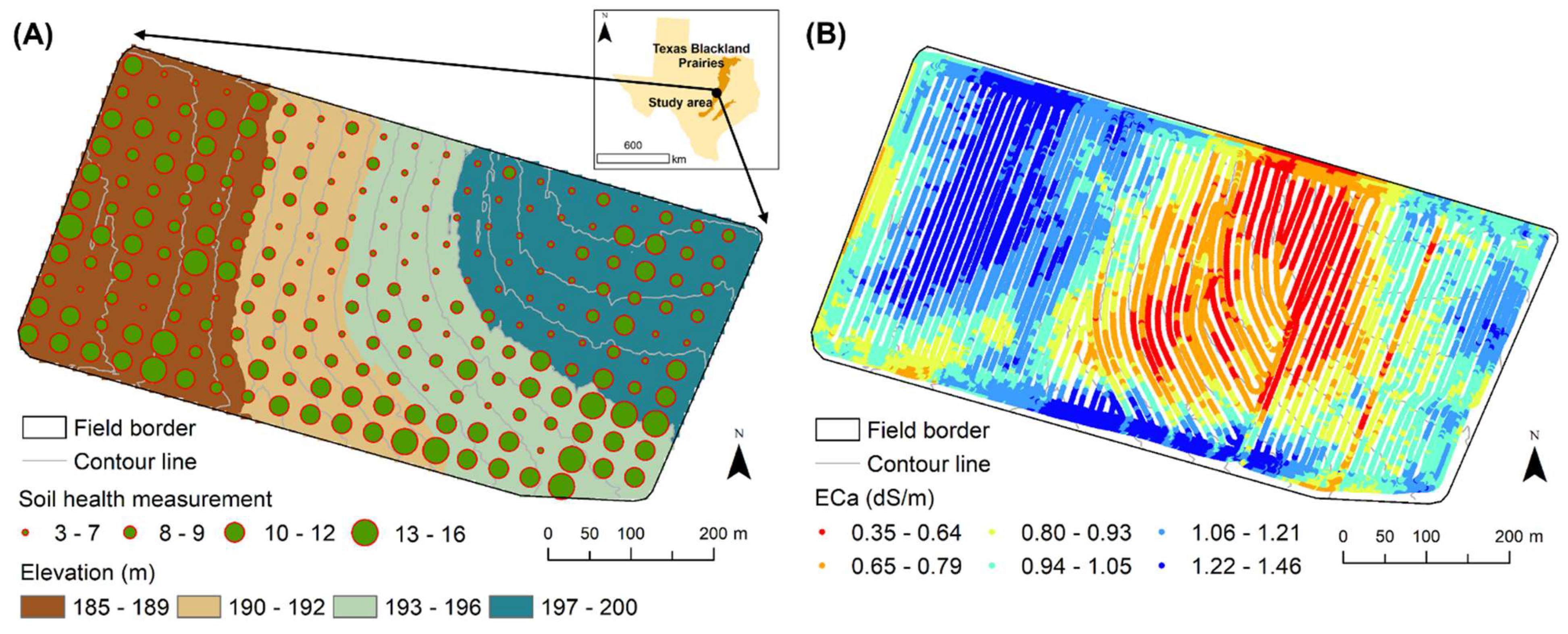
2.1. Site Description

The study site is located in the Blackland Prairies soils in Texas, USA (31°03′29.81″ N, 97°21′15.08″ W) (Figure 1A). The site is a rectangular-shaped agriculture field covering an area of about 27 ha. The field typically grows corn and cotton in rotation and has been under cultivation for >50 year. The field applies conservation practices, and the two most common around the area are terracing to reduce soil erosion and minimum tillage. Soils in the study area are >2 m deep and are developed on weathered chalk or clayey residuum from calcareous mudstone of the Cretaceous Age. These soils are classified as fine-silty, carbonatic, thermic Udorthentic Haplustolls (Austin silty clay series) or fine, smectitic, thermic, Udic Haplusterts (Houston Black clay series) according to Soil Taxonomy [37]. Surface elevation changes from 185 m in the west up to 200 m to the east with a moderate slope up to 3.5%. The climate is generally hot with an average annual high and low temperatures of 25 °C and 13 °C, respectively, with an average precipitation of about 937 mm annually.

2.2. Data Collection

Three sets of input data, namely, soil health indicators (one-day CO₂, organic C, organic N, and SHI), apparent electrical conductivity, and topographic data, were collected from the field, and are described below.

2.2.1. Soil Sampling and Measurement of Soil Health Indicators

The soil sampling scheme in the field was based on a 35 m × 35 m grid layout in which one undisturbed soil sample at each grid node (218 nodes in total) was collected with a hydraulic soil probe containing an insert. Geographical coordinates of each sample location were recorded using a hand-held global positioning system with an accuracy of 0.76 m. Soil samples from the top 15-cm soil depth were then brought to the USDA—ARS, Grassland, Soil, and Water Research Laboratory to determine soil health indicators, and SHI based on Haney Soil Health Tool [11]. Those indicators include one-day CO₂ evolution, water-extractable organic C (WEOC), and water-extractable organic N (WEON). One-day CO₂ evolution is the amount of CO₂ (mg/kg) released in the 24 h time period by soil microbes after the soil has been dried and rewetted, and it is a measure of the soil microbial activity related to soil fertility. The WEOC is the amount of organic C that is extracted from the soil with water, and it reflects the quantity of carbon in the soil that is readily available to microbes. Similarly, WEON is the amount of the total water-extractable nitrogen (WEN) minus the inorganic N that includes both nitrate and ammoniacal-nitrogen (NO₃-N and NH₄-N), and it can be easily broken down and released by soil microbes to the soil in readily plant-available inorganic N.

In the laboratory, soil samples were first oven-dried at 50 °C and crushed before sieving through a 2 mm mesh. From the sieved soil, a 4 g subsample was poured into a 50-mL centrifuge tube and was extracted with 40 mL de-ionized water. The extract was then analyzed for NO₃-N and NH₄-N using a Seal Analytical Rapid Flow Analyzer. The WEOC and WEN were determined using a Teledyne-Tekmar Apollo 9000 C: N analyzer and the WEON was derived as a difference between the total water-extractable N and nitrate-and ammoniacal-nitrogen (i.e., WEON = WEN–NH₄-N–NO₃–N). To determine one day CO₂ evolution, a 40 g sieved soil sample was put into a 50 mL perforated plastic beaker and was bought to a moisture level equivalent to field capacity solely through capillary action and the CO₂ released was determined by Licor 840 CO₂ detector [38]. All the laboratory procedures followed to determine soil health indicators can be found in Haney, Haney, Smith, Harmel, and White [11]. From these soil indicator values; SHI was derived as Equation (1). The SHI includes the weighted contribution of microbial activity, water-extractable organic C, and water-extractable organic N. The SHI score represents the overall health of the soil system and its value ranges between 0 and 50 or slightly over 50 in most agriculture systems, wherein scores > 7 are considered relatively good.

$$\mathrm{SHI}=\frac{\mathrm{One}-{\mathrm{day} \mathrm{CO}}_2}{\mathrm{WEOC}:\mathrm{WEON}}+\frac{\mathrm{WEOC}}{100}+\frac{\mathrm{WEON}}{10}$$

(1)

where one day CO₂ is the amount of CO₂ released in 24 h, WEOC as water-extractable organic C, and WEON as water-extractable organic N in mg/kg, the numbers 10 and 100 are the weighting factors.

2.2.2. Field Apparent Electrical Conductivity Survey and Mapping

A field survey was conducted in 2020 to collect ECa data across the field using a DualEM-1S sensor (DUALEM Products. Available online: https://dualem.com/products/ (accessed on 16 April 2022)). The DualEM-1S sensor works with the principles of electromagnetic induction. It has one transmitter (vertical dipole) and two receivers (vertical and horizontal dipole) separated by a distance of about 1 m. About 70% of the cumulative response of the horizontal configuration of the receiver comes from 0.5 m soil depth, whereas it corresponds to a depth of 1.5 m for the vertical configuration [39]. During the field operation, the sensor was tightly placed in a hard-core plastic sled and was dragged in the field with an all-terrain vehicle. A global positioning system (GPS Pathfinder Pro XRS) was connected to the sensor to record geographic coordinates in real-time. The sensor received power from the all-terrain vehicle and was connected to a field computer Yuma 2 Rugged Tablet. The communication between the sensor, GPS unit, and the field computer was acquired by running a Termite Software Program (Termite: a simple RS232 terminal. Available online: https://www.compuphase.com/software_termite.html (accessed on 16 April 2022))and its Geographic Information System (GIS) display by using Handheld GIS Mapping Software (HGIS GPS mapping. Available online: https://www.atsgps.com/hgis-gps-mapping.html (accessed on 16 April 2022)). The field survey was done in a single scan, and it took about 4.5 h to complete. There was a total of 85 drive-paths each placed roughly 5 to 8 m apart along the northeast-southwest direction of the field. ECa data were recorded every second that corresponded to a measuring distance of about 2.5 to 3 m along the drive path, making a total of 14,171 observations covering the entire study area. Each ECa measurement represented a GPS-recorded electrical conductivity in dS/m acquired for horizontal as well as the vertical configuration of the receiver; however, the present study only used the ECa data from its horizontal configuration, as it is more responsive to surface soil depth (~0.5 m) and properties.

Once the field scan was complete, recorded data in txt format were downloaded and imported to Microsoft Excel and to ArcGIS [40] for data cleaning and subsequent analysis. Data cleaning included removing data points falling outside the field boundary, overlapping points, out-of-drive-track points, negative points, and possible outliers determined as values falling outside this range [ECa value < (mean − 3 × standard deviations (SD)); > (mean + 3 × SD)]. A continuous ECa map at a grid size of 5 m × 5 m was generated by ordinary kriging as it outperformed inverse distance weighting, radial bias functions, and empirical Bayesian kriging methods in terms of prediction error (root mean squared error) based on leave-one-out cross-validation. A grid size of 5 m was selected for mapping to make the dimensions of the smallest spatial unit (the grid) compatible with the swath length of most farm equipment used in the field. Before the kriging operation, spatial autocorrelation of ECa observations (n = 14,171) was modelled with a variogram (nugget: 0.0, partial sill: 0.07, range: 320 m, model: spherical) considering 12 lags with a lag distance of 30 m in VESPER program [41].

2.2.3. Topographic Information

A digital elevation model (DEM) was compiled from light detection and ranging technology and the terrain attributes derived from the DEM were used as a source of topographic information in the study area. The DEM was downloaded from the USDA-Natural Resources Conservation Services, Geospatial Data Gateway website (Geospatial data gateway. Available online: ( https://gdg.sc.egov.usda.gov/GDGHome.aspx (accessed on 5 December 2021)). The DEM was originally compiled at a grid resolution of 1 m × 1 m, but it was resampled to a 5 m × 5 m grid for this study by applying the bilinear interpolation technique. Before deriving terrain attributes, the DEM was pre-processed by filling unnecessary sinks which would otherwise disrupt regular water flow and distribution on the soil surface. A total of 15 terrain attributes were derived from the DEM in SAGA GIS [42] platform and were used as predictors of soil health indicators, and SHI in the study area. The terrain attributes used were aspect (Aspect), elevation (Elevation), flow accumulation (FlowAccu), landscape position (Landforms), mid-slope position (Midslp), minimum curvature (Curvmin), multiresolution ridge top flatness (MRRTF), multiresolution valley bottom flatness (MRVBF), overland flow distance (Overlflw), wetness index (SAGAWI), slope gradient (Slope), slope height (Slopeht), slope-length factor (LSFactor), topographic position index (TPI), and valley depth (Valdep). More detail on these terrain attributes and their derivation can be found in Guo, et al. [43].

Table 1. Pearson’s correlation coefficient between measured soil properties, apparent electrical conductivity, and terrain attributes.

Name of Predictor Variable	Abbreviation Used	One Day CO2	Organic C	Organic N	Soil Health Index
Aspect	Aspect	−0.13 **	0.05	−0.04	−0.10
Apparent electrical conductivity	ECa	0.47 ***	0.07	−0.11	0.37 ***
Elevation	Elevation	−0.24 ***	−0.22 ***	−0.19 **	−0.27 ***
Flow accumulation	FlowAccu	−0.17 **	−0.07	−0.14 **	−0.16 **
Landscape position	Landforms	−0.36 ***	−0.31 ***	−0.28 ***	−0.40 ***
Mid-slope position	Midslp	0.28 ***	0.09	0.02	0.24 ***
Minimum curvature	Curvmin	0.16 **	0.11	0.11	0.16 **
Multiresolution ridge top flatness	MRRTF	−0.06	−0.20 ***	−0.24 ***	−0.12
Multiresolution valley bottom flatness	MRVBF	0.50 ***	0.31 ***	0.23 ***	0.49 ***
Overland flow distance	Overlflw	0.11	−0.10	−0.03	0.07
Wetness index	SAGAWI	0.52 ***	0.44 ***	0.44 ***	0.57 ***
Slope gradient	Slope	−0.36 ***	−0.20 ***	−0.12	−0.33 ***
Slope height	Slopeht	−0.15 **	−0.21 ***	−0.25 ***	−0.20 ***
Slope-length factor	LSFactor	−0.14 **	−0.14 **	−0.09	−0.15 **
Topographic position index	TPI	−0.44 ***	−0.27 ***	−0.24 ***	−0.44 ***
Valley depth	Valdep	0.28 ***	0.21 ***	0.25 ***	0.30 ***

***: significant at p < 0.0001; **: significant at p < 0.01.

lists all the terrain attributes and ECa and their correlation with one-day CO₂, organic C, organic N, and SHI from the study area.

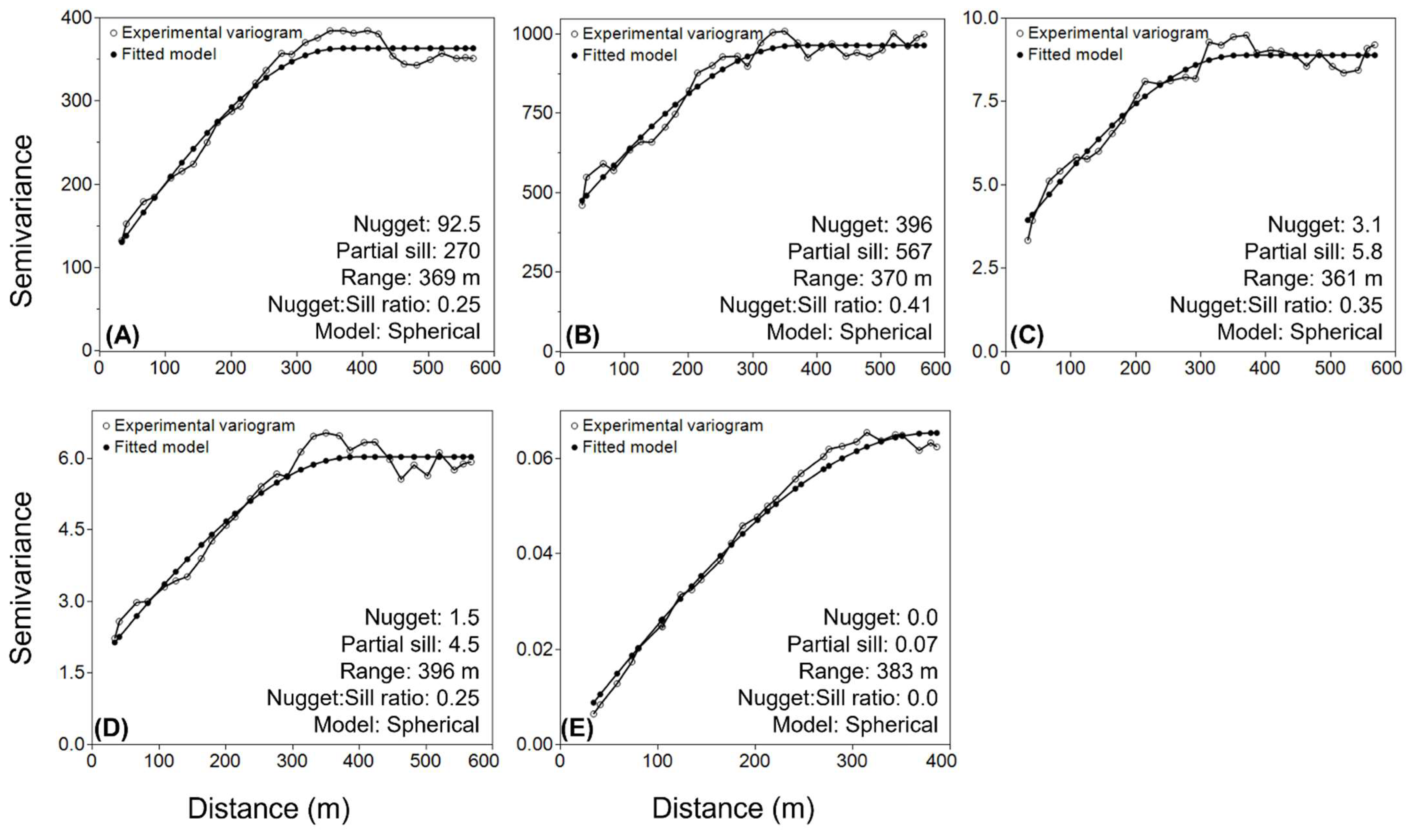
2.3. Assessment of Autocorrelation and Spatial Dependency

Spatial autocorrelation of one-day CO₂, organic C, organic N, SHI, and ECa was investigated using variograms that plot semivariance among observation pairs against their separation distances (Equation (2)). It measures the average degree of dissimilarity between unsampled values and a nearby data value [44] and thus can describe autocorrelation among observations at various distances. We calculated omnidirectional experimental variograms of measured properties following Equation (2) and modeled its spatial characteristics using three different variogram models (Spherical model, Exponential model, and Gaussian model). The variogram parameters nugget (C₀), partial sill (C₁), and range of the variogram (a) from the best-fitted model among the three tested that provided the lowest value of Akaike Information Criteria were recorded and were used to characterize spatial autocorrelation or spatial dependence of the measured properties using nugget: sill ratio (NSR). The NSR represents a contribution of the nugget to the overall spatial structure of the variogram and it can be calculated as NSR = C₀/(C₀ + C₁). The NSR tells how well the measured property is spatially dependent or autocorrelated (NSR < 0.25, strong; 0.25 < NSR > 0.75, moderate; and NSR > 0.75, weak) [45]. The experimental variograms were calculated considering 30 lags with a lag distance of 20 m for all measured properties. Lags are the distances between observation pairs at which the variogram is calculated. Variogram calculation and model fitting was performed in the VESPER program [41].

$$\mathsf{\gamma }\left(\mathrm{h}\right)=\frac{1}{2\mathrm{N}\left(\mathrm{h}\right)}{\displaystyle \sum }_{\mathrm{a}=1}^{\mathrm{N}\left(\mathrm{h}\right)}{\left\{\mathrm{z}\left({\mathrm{x}}_{\mathrm{a}}+\mathrm{h}\right)-\mathrm{z}\left({\mathrm{x}}_{\mathrm{a}}\right)\right\}}^2$$

(2)

where, γ_(h) is the variogram for a distance h(lag) between observations z(x_a) and z(x_a + h) with N_(h) the number of observation pairs separated by h.

2.4. Spatial Prediction, Mapping, and Model Validation

Prediction of one-day CO₂, organic C, organic N, SHI, and ECa and its mapping across the study area was performed with a machine learning technique—Random Forest. The RF model was employed using a package ‘randomForest’ in the R environment [46], with three different parameters defined in the model: the number of trees (ntree) set to be 500, the minimum number of data points be used in each terminal node (nodesize) set to be 1, and the number of variables tried at each node (mtry) was 4 determined with ‘tuneRF’ function. The model also quantified the relative importance (RI) of predicting variables based on the ranking of percentage increase in prediction error (mean squared error) (%IncMSE) on its removal from the model. Before executing the RF model, point observations were randomly split into training (75% of the data) for model calibration and test datasets (25% of the data) for model performance evaluation. The mean and SD values of the measured properties in training and test datasets were comparable. A correlation matrix of one day CO₂, organic C, organic N, and SHI and predictor variables was generated and the variables that were at least significant at p value of <0.01 for each property were used in the RF models for subsequent predictions. Once the predictions were made, the maps were exported to ArcGIS [40] for necessary map edits and layout.

The performance of the prediction models was evaluated on both the calibration as well as the validation data sets using the statistical indices of R², Lin’s Concordance Correlation Coefficient (LCCC), root mean squared error (RMSE), and mean error (ME). The LCCC was calculated as Equation (3), the calculation of the remaining indices could be found elsewhere, e.g., [47].

$$\mathrm{LCCC}=\frac{2{\mathsf{\rho }\mathsf{\sigma }}_{\mathrm{Y}}{\mathsf{\sigma }}_{\mathrm{X}}}{{\mathsf{\sigma }}_{\mathrm{Y}}^2+{\mathsf{\sigma }}_{\mathrm{X}}^2+{\left(\overline{\mathrm{Y}}-\overline{\mathrm{X}}\right)}^2}$$

(3)

where $\overline{\mathrm{X}}$ and $\overline{\mathrm{Y}}$ are the mean of the observed (X) and predicted values (Y), $\mathsf{\rho }$ is the correlation coefficient between observations and predictions, ${\mathsf{\sigma }}_{\mathrm{X}}$ and ${\mathsf{\sigma }}_{\mathrm{Y}}$ as corresponding standard deviations, and ${\mathsf{\sigma }}_{\mathrm{X}}^2$ and ${\mathsf{\sigma }}_{\mathrm{Y}}^2$ corresponding variances.

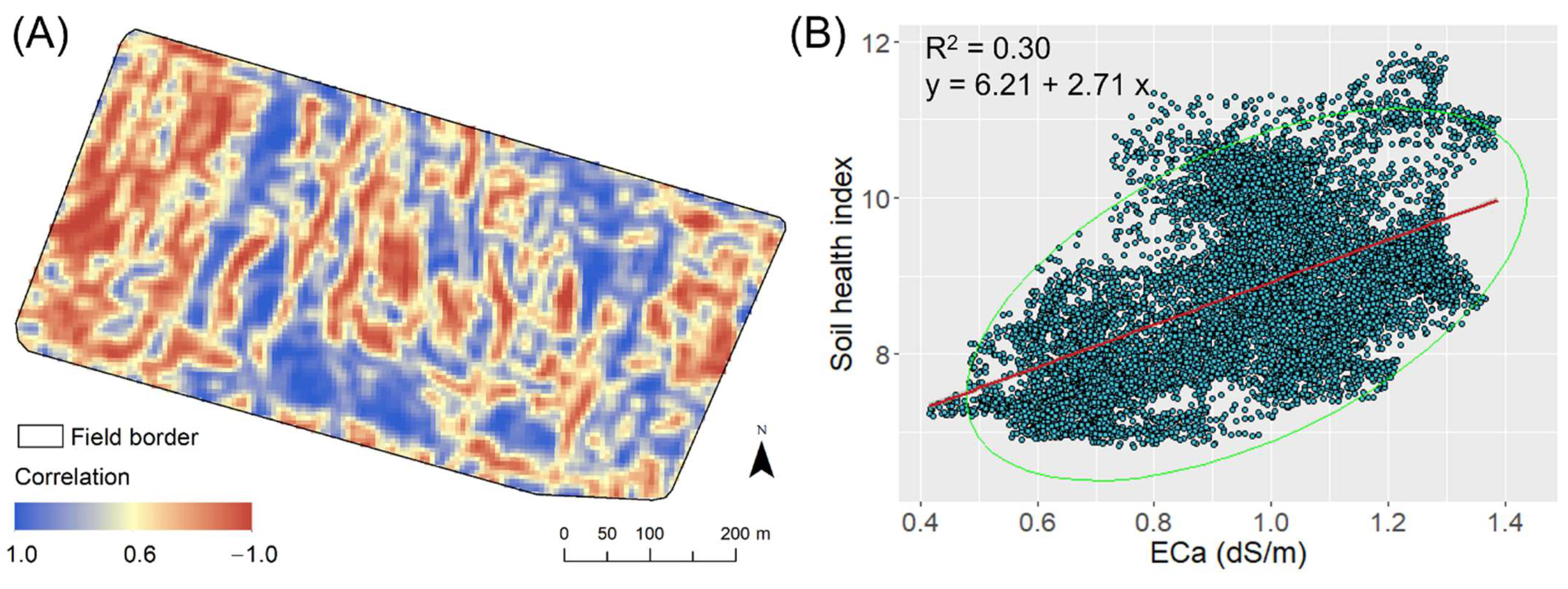
2.5. Correlation between ECa and Soil Health Index and Its Mapping

Spatial correlation between ECa and SHI maps was quantified using a local correlation between two maps [48], and the values were mapped across the study area at 5 m spatial resolution. Around each pixel of the raster, a 3 × 3 pixel neighborhood was defined to record local correlation using the ‘cor’ function, and the operation was repeated throughout the raster using the ‘focal’ function in the R environment [46]. Further, an empirical relationship between ECa and SHI was established using a linear model where SHI was used as a dependent variable on ECa for each predicted pixel from the map. The linear equation could then be used to predict SHI from easy to obtain ECa data.

3. Results

3.1. Descriptive Summary of Observation Data

Summary statistics of one-day CO₂, organic C, organic N, SHI, and ECa for the measurement locations are listed in

Table 2. Summary statistics of soil health indicators, soil health index, and apparent electrical conductivity measured at sample locations (n = 218).

	One Day CO2 (mg/kg)	Organic C (mg/kg)	Organic N (mg/kg)	Soil Health Index	ECa (dS/m)
Mean	42.7	154	11.7	8.5	1.0
SD	17.5	29.1	2.8	2.2	0.2
Skewness	1.0	0.6	−0.4	0.8	−0.2
Kurtosis	1.8	0.6	0.2	1.1	−0.8
CV %	41.0	18.9	24.0	26.3	21.8
Minimum	9.9	59.0	3.9	2.6	0.5
Maximum	123	242	20.1	16.4	1.4
Median	40.3	151	12.0	8.2	1.0
IQR	24.0	36.0	3.5	2.8	0.3

SD: standard deviation; CV: coefficient of variation; IQR: Inter-quartile range; ECa: apparent electrical conductivity.

. One day CO₂ measurements ranged from 9.9 to 123 mg/kg with a mean of 42.7 (±17.5 SD). Average organic C and organic N were 154 and 11.7 mg/kg, respectively, with their corresponding coefficient of variation (CV) of 18.9, and 24%. Similarly, SHI ranged from 2.6 to 16.6 with a mean of 8.5 (±2.2 SD), and that of ECa from 0.5 to 1.5 dS/m with a mean of 1.0 ((±0.2 SD). Among all properties, one-day CO₂ had the highest CV (41%) followed by SHI, and organic C had the smallest CV (18.9%) of all. All properties data had positive skewness coefficients except for organic N and ECa which were slightly negatively skewed with skewness coefficients of −0.4, and −0.2, respectively.

3.2. Spatial Autocorrelation

The experimental variogram of the measured properties was best modeled with a spherical variogram as the model showed the lowest value of Akaike Information Criteria among the tested models—Spherical, Exponential, and Gaussian models (Figure 2). The range of the variogram of one-day CO₂, organic C, and organic N was between 360–370 m, and NSR between 0.25 and 0.41 showing a strong to moderate spatial dependence of these properties. Similarly, a strong spatial dependence was observed for SHI, which had a range of 396 m, and a partial sill of 4.5. Among these four properties, SHI had the lowest nugget variance and organic C had the highest nugget of all. ECa was strongly spatially dependent with a nugget variance of zero, and a range of 383 m.

3.3. Correlation of Soil Properties with Predictors

A Pearson’s correlation coefficient of one-day CO₂, organic C, organic N, and SHI with predicting variables that included terrain attributes and ECa is listed in Table 1 with their corresponding level of significance. Among the 16 predictors, 14 predictors were significantly correlated (p-value < 0.01) with one-day CO₂, 10 predictors with organic C, 9 predictors with organic N, and 13 predictors with SHI, respectively. The predictors that were not significantly correlated with one-day CO₂ were MRRTF and Overlflw. Similarly, predictors that were not significant with organic C were Aspect, ECa, FlowAccu, Midslp, Curvmin, and Overlflw. The same predictors that were not significant with organic C except FlowAccu were also non-significant for organic N. Two additional predictors namely, Slope and LSFactor were found non-significant to predict organic N as well; however, both were significantly correlated with organic C. In the case of SHI, all predictors except Aspect, MRRTF, and Overlflw were significantly correlated.

Among the predictors, ECa was positively correlated with one-day CO₂ (r = 0.47), and SHI (r = 0.37), but was weakly correlated with organic C (r = 0.07) and organic N (r = −0.11). Elevation, on the other hand, was negatively correlated with all properties with r ranging from −0.19 for organic N to −0.27 for SHI. There was a strong positive correlation of one-day CO₂ with MRVBF (r = 0.50), and SAGAWI (r = 0.52), and a negative correlation with TPI (r = −0.44), Landforms (r = −0.36), and Slope (r = −0.36). Similarly, organic C was strongly negatively correlated with Landforms but positively correlated with SAGAWI (r = 0.44), which was positively correlated with organic N (r = 0.44). There was a strong positive correlation of SHI with MRVBF (r = 0.49), SAGAWI (r = 0.57); and a negative correlation with Landforms (r = −0.40), and TPI (r = −0.44).

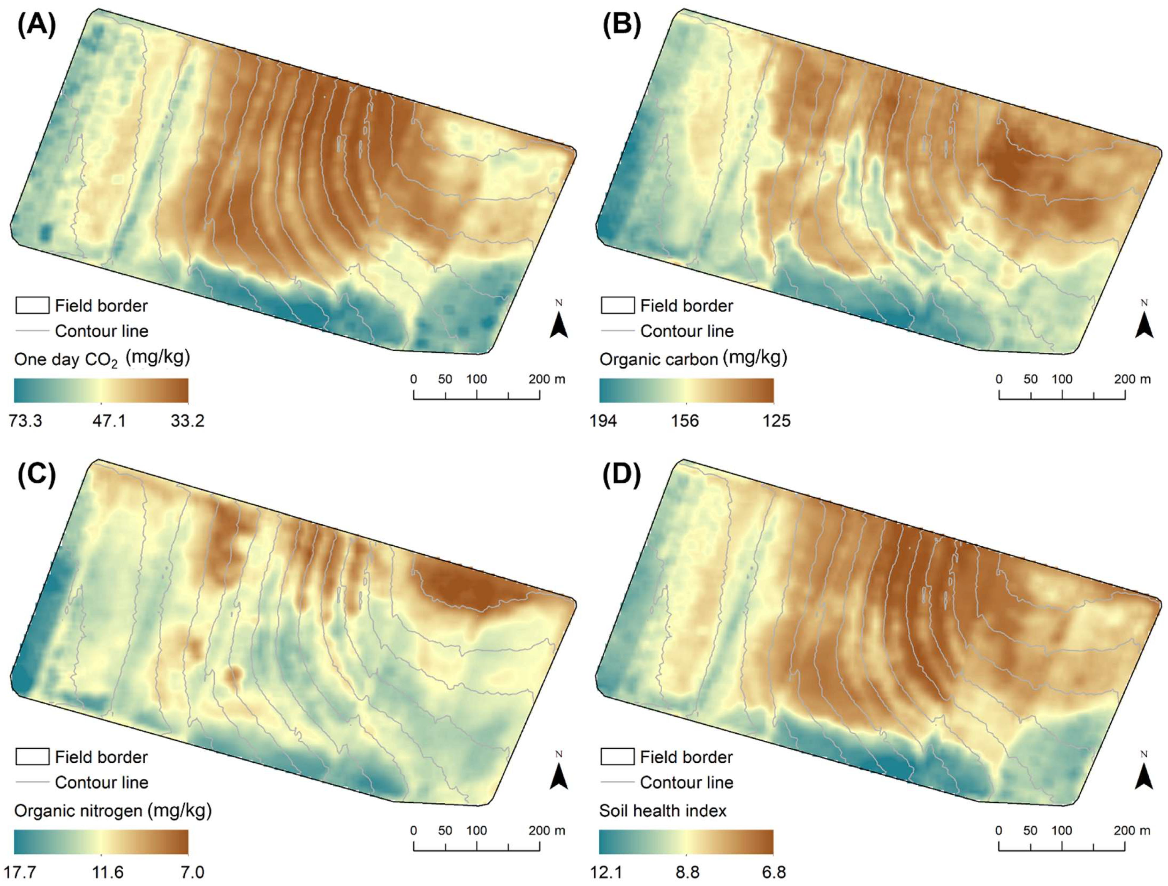
3.4. Model Performance and Predicted Maps

The RF model used to predict and map soil health indicators and SHI was evaluated on 25% set-aside data that were not used in model calibration, and

Table 3. Performance evaluation of prediction model on train (75%) and test (25%) dataset.

	R2		LCCC		RMSE		ME
	Train	Test	Train	Test	Train	Test	Train	Test
One-day CO2	0.90	0.48	0.93	0.63	4.72	10.15	0.07	−0.16
Organic C	0.85	0.24	0.91	0.33	8.48	20.29	0.05	0.34
Organic N	0.87	0.41	0.91	0.54	1.01	3.01	0.00	0.03
Soil Health Index	0.90	0.47	0.93	0.52	0.61	1.38	0.00	0.00

R²: coefficient of determination; LCCC: lin’s concordance correlation coefficient; RMSE: root mean squared error; ME: mean error.

lists model evaluation results for both training and test datasets. The predicted R² value ranged from 0.85 to 0.90 for training data, and from 0.24 to 0.48, respectively, for the test data; one-day CO₂ had the highest R², and organic C had the lowest R² of all. The model produced the highest LCCC for one-day CO₂ and the lowest RMSE value for SHI, and the lowest LCCC and the highest RMSE for the prediction of organic C in the test data set. The ME statistics showed that the model was negatively biased to predict one-day CO₂. Overall, the RF model showed that the SHI was best predicted with the higher value of R² and LCCC and the lower value of RMSE, and organic C was least predicted with the lowest value of R² and LCCC and the highest value of RMSE (Table 3).

The predicted map of one-day CO₂, organic C, organic N, and SHI are shown in Figure 3, and their corresponding important predictors are shown in Figure 4, respectively. These maps were generated by using the RF model in which only the significant predictors of each property (Table 1) were used in their subsequent predictions. Based on the predicted maps, the investigated field seems variable in terms of soil health indicators and SHI distribution; CVs of these properties ranged between 8% and 20%. Among all properties, organic C distribution in the field was least variable (mean = 157 mg/kg; CV = 8.2%) and organic N was moderately variable (mean = 11.7 mg/kg; CV = 13%). The maps showed that a major portion of the central part of the field had a lower level of one-day CO₂ and organic C content resulting in a lower SHI value in that area compared to the rest of the field. On the other hand, most of the southern part of the field had higher values of those properties including organic N. Specific to organic N which was higher in the lower 3 quarters of the field, its maximum value was mapped from the southernmost part, and in the western corner of the field. These maps also showed the influence of field terracing on the spatial distribution of measured properties across the field (Figure 3).

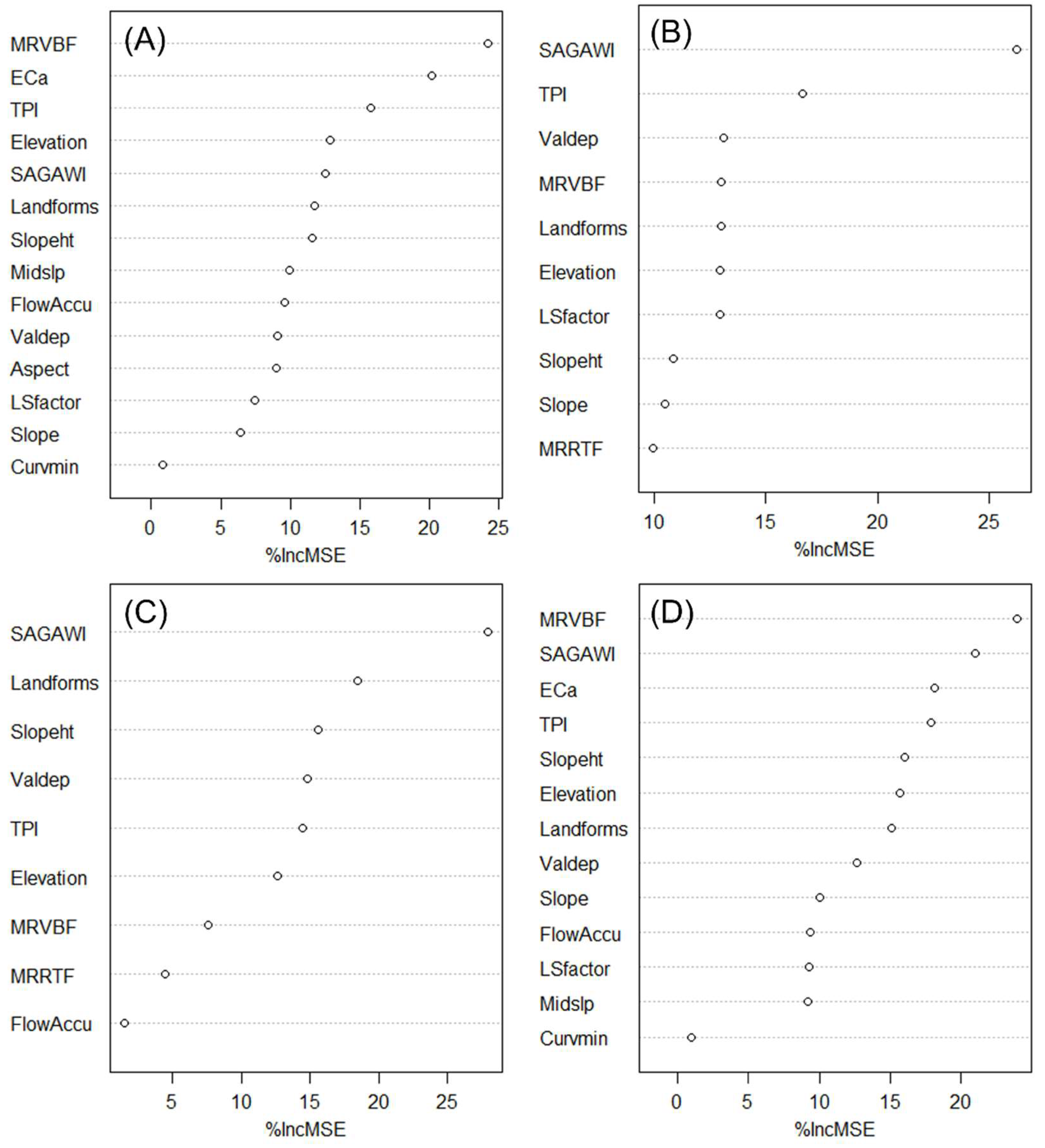
3.5. Important Predictors for Soil Health

Among the 16 predictors (Table 2), SAGAWI was ranked in the list of top five predictors of all properties indicating its higher influence on the spatial distribution of these properties in the study area (Figure 4). The RI of SAGAWI ranged between 13% for one-day CO₂ to 29% for organic C and organic N prediction. Similarly, ECa was among the top three predictors of one-day CO₂ and SHI for which the highest RI of nearly 21% was observed. However, ECa was not considered a good predictor of organic C and organic N distribution, even though it had some correlation with those properties. Predictors such as Curvmin, slope, FlowAccu, and MRRTF were less important compared to multiresolution valley bottom flatness, TPI, Landforms, and slope height to predict soil health indicators and SHI. Predictors like multiresolution valley bottom flatness, SAGAWI, and TPI were the top terrain attributes to predict one-day CO₂, organic C, organic N, and SHI in the study area. Overall, the spatial distribution of soil health indicators and SHI in the study area was greatly influenced by ECa and local topography and their level of influence depended on the properties considered (Figure 4).

3.6. Relationship between ECa and soil Health Index

Spatial correlation between SHI and ECa maps based on each predicted pixel quantified and mapped as in Figure 5A and the linear relationship between them is shown in 5B, respectively. There was a correlation of about 0.55 between ECa and SHI based on all pixels and its distribution showed some patchy patterns across the field. The western part of the field showed a lower or negative correlation between ECa and SHI compared to the rest of the field; the central and the eastern part of the field showed a mixed low and high correlation between ECa and SHI. Based on the linear relationship between SHI and ECa, 30% of SHI variability was explained by ECa only, and that the former could be predicted by ECa with an equation: y = 6.21 + 2.71x.

4. Discussion

In this study, a 35 m × 35 m grid design was applied to identify sampling locations for mapping within-field soil health status across a field. As reported in Adhikari, Smith, Collins, Haney, and Wolfe [35], the selected grid size of 35 m × 35 m and the number of samples collected were representative of the study area to capture field variability, as the grid size was smaller than the range of the modeled variograms of measured soil properties [49]. Furthermore, grid sampling is a widely used soil sampling scheme in field-scale soil attribute mapping, e.g., [50,51] because of its simplicity and potential for greater efficiency [52]. Grid samplings are useful to access within-field variations in plant-available nutrients and facilitate site-specific management [53,54]. Spatial autocorrelation of soil health indicators and SHI including ECa was investigated with geostatistical methods (i.e., variogram) which are common in spatial studies in soil and agronomic research [55]. As suggested by [56], the spherical model is a common variogram model to describe the autocorrelation of soil properties, and our study reported the same as the experimental variogram of all properties were best modeled by a spherical model. We observed that one-day CO₂, SHI, and ECa had a strong spatial dependence, and organic C and organic N had a moderate dependence in the study area. A strong spatial dependence of SHI at a field scale was previously reported by Amirinejad, et al. [57] in which the variogram range of organic C and SHI varied between 300–380 m, similar to the variogram ranges observed in this study. The range values of one-day CO₂, organic C, and organic N were between 360–370 m, and it is the average distance to which those properties are correlated in the field [58].

Spatial variability in soil properties affects crop performance, yield, and adoption of site-specific management practices. The study site showed a moderate to a high degree of variability (i.e., CV 15–35%: moderate; CV > 35%: high [59] as the CV of measured soil properties including SHI, and ECa ranged between 18.9 to 41% (Table 2). The spatial variability of those properties was predicted and mapped with a RF model which is becoming popular in field-scale soil properties mapping because of its higher prediction performance, among other benefits. Studies by Schmidt, et al. [60] and Zhang, Ji, Saurette, Easher, Li, Shi, Adamchuk, and Biswas [32] found a higher and more consistent performance of the RF model compared to regression tree and generalized linear model in predicting soil properties at field level; our results are consistent with these findings as we observed a similar model performance (R² as high as 0.90). However, a recent study from Denmark found the performance of kriging (R² = 0.90) as high as the RF model (R² = 0.91) in predicting field-scale variability of soil organic matter [50]. Authors argued that the higher performance of kriging might be due to a high sampling density (20 m × 20 m grid sampling scheme) in their field.

The present study used a range of terrain attributes and ECa which were collected on-the-go as predictors of one-day CO₂, organic C, organic N, and SHI. Research showed that collecting ECa data on the go is an efficient way of capturing field variability as ECa is mostly related to soil physicochemical properties (e.g., porosity, soil moisture, salinity, cation composition, cation exchange capacity, ionic strength, particle size distribution, particle shape and orientation, wettability) [61], and it can be collected intensively in an easy and inexpensive way [62,63]. Due to their correlation with soil properties, ECa and terrain attributes are widely used in spatial prediction and mapping of soils properties at the field scale, e.g., [51,64,65,66,67]. Among the predictors used, we found a weak correlation of ECa with organic C, and organic N, whereas it was highly correlated with SHI and one-day CO₂. Our study highlighted the importance of terrain attributes such as SAGAWI, MRVBF, and TPI in predicting soil health indicators in the study area. SAGAWI had the highest influence on Organic C, Organic N, and SHI (RI > 25%) suggesting that the field areas that tend to remain moist or low-lying areas had a strong and positive (Table 1) influence on these properties. A positive influence of wetness index on soil carbon distribution was also reported in other studies, e.g., [50,68]. As low-lying or concave areas in the field tend to accumulate organic matter due to erosion from upslope areas and favor slow decomposition of organic matter [69,70], terrain attributes like SAGAWI, MRVBF, and Valdep have a high potential to predict soil carbon and nitrogen distribution in those areas. We also observed the influence of field terracing on soil properties distribution (Figure 3). Those terraces were built to reduce soil erosion, and increase infiltration 30–40 year ago, which might have influenced field hydrology and soil and nutrient transport [71]. The terrain attributes we used for prediction were able to identify those terracing signatures and perhaps captured their influence on soil properties variations across the field.

The correlation map between ECa and SHI shows a pixel-by-pixel relationship between these properties and it could provide a lot more information in the spatial context. This could be very useful in within-field soil variability assessment and for site-specific management decisions as it shows a direct relationship between these properties from every paddock of the field. Establishing an empirical relationship between ECa and SHI is helpful, as it highlights the potential of on-the-go sensing to estimate SHI in the field easily and efficiently with a minimum cost.

5. Conclusions

This study was conducted to quantify and map within-field variability of the soil health status of Blackland prairies soils in Texas. Two hundred and eighteen topsoil samples were collected and analyzed for one-day CO₂, organic C, organic N, and soil health index. A High-resolution (5 m × 5 m grid) map of each property was generated using a random forest model in which terrain attributes and ECa data were used as predictors. Furthermore, the spatial correlation between ECa and SHI was mapped and a linear relationship between them was established. Results showed that one-day CO₂, organic C, and organic N, SHI, and ECa data were moderate to strongly spatial dependent in the study area, and the range of this dependency was between 259 to 396 m. The ECa was strongly positively correlated with one-day CO₂, and SHI, whereas it was weakly correlated with organic C and organic N. There was a strong positive correlation between one-day CO₂, organic C, and organic N, and SHI and SAGAWI, and a strong negative correlation with TPI. Based on the predicted maps, average values of one-day CO₂, and SHI were 47.1 mg/kg (±7.9 SD), and 8.9 (±1.2 SD), respectively. The field shows high variability in terms of SHI. The ECa, SAGAWI, MRVBF, and TPI were among the top predictors of soil health indicators, and SHI in the study area, while ECa was a good predictor of one-day CO₂, and SHI, but not for organic C and organic N. Validation of the RF model showed a higher prediction performance for one-day CO₂ and SHI but a lower performance for organic C. The ECa and SHI maps were correlated (r = 0.55), and the latter could be fairly estimated with ECa with a linear function y = 6.21 + 2.71x. There was a noticeable variation in the selected soil health indicators, and SHI in the study area at within-field scale, and such variation could play a role in yield variations across the field. We recommend using topography and ECa to predict soil health indicators and soil health indexes. Further, SHI could be fairly estimated with ECa data that could be collected on-the-go efficiently with minimum cost; however, it needs to be tested in other fields as well. We believe the high-resolution predicted maps of soil health indicators, and SHI including the correlation map between ECa and SHI could be useful in fine-tuning SSCM applications.

References

1. Doran, J.W.; Zeiss, M.R. Soil health and sustainability: Managing the biotic component of soil quality. Appl. Soil Ecol. 2000, 15, 3–11. [Google Scholar] [CrossRef] [Green Version]
2. Doran, J.W.; Safley, M. Defining and accessing soil health and sustainable productivity. In Biological Indicators of Soil Health; Pankhurst, C.E., Doube, B.M., Gupta, V.V.S.R., Eds.; CAB International: New York, NY, USA, 1997; pp. 1–28. [Google Scholar]
3. Kibblewhite, M.; Ritz, K.; Swift, M. Soil health in agricultural systems. Philos. Trans. R. Soc. B Biol. Sci. 2008, 363, 685–701. [Google Scholar] [CrossRef] [Green Version]
4. Maharjan, B.; Das, S.; Acharya, B.S. Soil Health Gap: A concept to establish a benchmark for soil health management. Glob. Ecol. Conserv. 2020, 23, e01116. [Google Scholar] [CrossRef]
5. Magdoff, F. Concept, components, and strategies of soil health in agroecosystems. J. Nematol. 2001, 33, 169. [Google Scholar] [PubMed]
6. Brevik, E.C. Soil health and productivity. In Soils, Plant Growth Crop Production; Verheye, W.H., Ed.; EOLSS Publications: Oxford, UK, 2010; Volume 1, p. 106. [Google Scholar]
7. Ditzler, C.A.; Tugel, A.J. Soil quality field tools: Experiences of USDA-NRCS Soil Quality Institute. Agron. J. 2002, 94, 33–38. [Google Scholar] [CrossRef]
8. Soil Health Institute. North American Project to Evaluate Soil Health Measurements. Available online: https://soilhealthinstitute.org/north-american-project-to-evaluate-soil-health-measurements/ (accessed on 7 October 2020).
9. Moebius-Clune, B.N.; Moebius-Clune, D.J.; Gugino, B.K.; Idowu, O.J.; Schindelbeck, R.R.; Ristow, A.J.; van Es, H.M.; Thies, J.E.; Shayler, H.A.; McBride, M.B.; et al. Comprehensive Assessment of Soil Health—The Cornell Framework; Edition 3.2; Cornell University: Geneva, NY, USA, 2016. [Google Scholar]
10. Schindelbeck, R.R.; van Es, H.M.; Abawi, G.S.; Wolfe, D.W.; Whitlow, T.L.; Gugino, B.K.; Idowu, O.J.; Moebius-Clune, B.N. Comprehensive assessment of soil quality for landscape and urban management. Landsc. Urban Plan. 2008, 88, 73–80. [Google Scholar] [CrossRef] [Green Version]
11. Haney, R.L.; Haney, E.B.; Smith, D.R.; Harmel, R.D.; White, M.J. The soil health tool-Theory and initial broad-scale application. Appl. Soil Ecol. 2018, 125, 162–168. [Google Scholar] [CrossRef]
12. Idowu, O.J.; van Es, H.M.; Abawi, G.S.; Wolfe, D.W.; Schindelbeck, R.R.; Moebius-Clune, B.N.; Gugino, B.K. Use of an integrative soil health test for evaluation of soil management impacts. Renew. Agric. Food Syst. 2009, 24, 214–224. [Google Scholar] [CrossRef] [Green Version]
13. Karlen, D.L.; Andrews, S.S.; Wienhold, B.J.; Zobeck, T.M. Soil quality assessment: Past, present and future. J. Integr. Biosci. 2008, 6, 12. [Google Scholar]
14. Yost, M.A.; Veum, K.S.; Kitchen, N.R.; Sawyer, J.E.; Camberato, J.J.; Carter, P.R.; Ferguson, R.B.; Fernandez, F.G.; Franzen, D.W.; Laboski, C.A.; et al. Evaluation of the Haney Soil Health Tool for corn nitrogen recommendations across eight Midwest states. J. Soil Water Conserv. 2018, 73, 587–592. [Google Scholar] [CrossRef] [Green Version]
15. Beckett, P.; Webster, R. Soil variability: A review. Soils Fertil. 1971, 34, 1–15. [Google Scholar]
16. Cline, M.G.J.S.S. Principles of soil sampling. Soil Sci. 1944, 58, 275–288. [Google Scholar] [CrossRef]
17. Bourennane, H.; Nicoullaud, B.; Couturier, A.; King, D. Exploring the Spatial Relationships Between Some Soil Properties and Wheat Yields in Two Soil Types. Precis. Agric. 2004, 5, 521–536. [Google Scholar] [CrossRef]
18. Eghball, B.; Schepers, J.S.; Negahban, M.; Schlemmer, M.R. Spatial and Temporal Variability of Soil Nitrate and Corn Yield. Agron. J. 2003, 95, 339–346. [Google Scholar] [CrossRef]
19. Miao, Y.; Mulla, D.J.; Robert, P.C. Identifying important factors influencing corn yield and grain quality variability using artificial neural networks. Precis. Agric. 2006, 7, 117–135. [Google Scholar] [CrossRef]
20. Rodrigues, M.S.; Cora, J.E.; Fernandes, C. Soil sampling intensity and spatial distribution pattern of soils attributes and corn yield in no-tillage system. Eng. Agric. 2012, 32, 851–864. [Google Scholar] [CrossRef] [Green Version]
21. Bouma, J.; Stoorvogel, J.; Van Alphen, B.; Booltink, H. Pedology, precision agriculture, and the changing paradigm of agricultural research. Soil Sci. Soc. Am. J. 1999, 63, 1763–1768. [Google Scholar] [CrossRef]
22. Geypens, M.; Vanongeval, L.; Vogels, N.; Meykens, J. Spatial variability of agricultural soil fertility parameters in a gleyic podzol of Belgium. Precis. Agric. 1999, 1, 319–326. [Google Scholar] [CrossRef]
23. Adhikari, K.; Carre, F.; Toth, G.; Montanarella, L. Site Specific Land Management: General Concepts and Applications; Office for Official Publications of the European Communities: Luxembourg, 2009; pp. 1–60. [Google Scholar]
24. Corwin, D.L.; Lesch, S.M. Application of Soil Electrical Conductivity to Precision Agriculture. Agron. J. 2003, 95, 455–471. [Google Scholar] [CrossRef]
25. Corwin, D.L.; Scudiero, E. Field-scale apparent soil electrical conductivity. Soil Sci. Soc. Am. J. 2020, 84, 1405–1441. [Google Scholar] [CrossRef]
26. Bronson, K.F.; Booker, J.D.; Officer, S.J.; Lascano, R.J.; Maas, S.J.; Searcy, S.W.; Booker, J. Apparent Electrical Conductivity, Soil Properties and Spatial Covariance in the U.S. Southern High Plains. Precis. Agric. 2005, 6, 297–311. [Google Scholar] [CrossRef]
27. Rhoades, J.D.; Corwin, D.L. Soil electrical conductivity: Effects of soil properties and application to soil salinity appraisal. Commun. Soil Sci. Plant Anal. 1990, 21, 837–860. [Google Scholar] [CrossRef]
28. Earl, R.; Taylor, J.C.; Wood, G.A.; Bradley, I.; James, I.T.; Waine, T.; Welsh, J.P.; Godwin, R.J.; Knight, S.M. Soil Factors and their Influence on Within-field Crop Variability, Part I: Field Observation of Soil Variation. Biosyst. Eng. 2003, 84, 425–440. [Google Scholar] [CrossRef] [Green Version]
29. McBratney, A.B.; Santos, M.L.M.; Minasny, B. On digital soil mapping. Geoderma 2003, 117, 3–52. [Google Scholar] [CrossRef]
30. Lagacherie, P. Digital Soil Mapping: A State of the Art. In Digital Soil Mapping with Limited Data; Hartemink, A.E., McBratney, A., Mendonça-Santos, M.d.L., Eds.; Springer: Dordrecht, The Netherlands, 2008; pp. 3–14. [Google Scholar] [CrossRef]
31. Bishop, T.F.A.; McBratney, A.B. A comparison of prediction methods for the creation of field-extent soil property maps. Geoderma 2001, 103, 149–160. [Google Scholar] [CrossRef]
32. Zhang, Y.; Ji, W.; Saurette, D.D.; Easher, T.H.; Li, H.; Shi, Z.; Adamchuk, V.I.; Biswas, A. Three-dimensional digital soil mapping of multiple soil properties at a field-scale using regression kriging. Geoderma 2020, 366, 114253. [Google Scholar] [CrossRef]
33. Breiman, L. Random forests. Mach. Learn. 2001, 45, 5–32. [Google Scholar] [CrossRef] [Green Version]
34. Biau, G.; Scornet, E. A random forest guided tour. Test 2016, 25, 197–227. [Google Scholar] [CrossRef] [Green Version]
35. Adhikari, K.; Smith, D.R.; Collins, H.; Haney, R.L.; Wolfe, J.E. Corn response to selected soil health indicators in a Texas drought. Ecol. Indic. 2021, 125, 107482. [Google Scholar] [CrossRef]
36. Caudle, C.; Osmond, D.; Heitman, J.; Ricker, M.; Miller, G.; Wills, S. Comparison of soil health metrics for a Cecil soil in the North Carolina Piedmont. Soil Sci. Soc. Am. J. 2020, 84, 978–993. [Google Scholar] [CrossRef] [Green Version]
37. Soil Survey Staff. Keys to Soil Taxonomy, 11th ed.; US Department of Agriculture, Natural Resources Conservation Service: Washington, DC, USA, 2010.
38. Haney, R.L.; Haney, E.B.; White, M.J.; Smith, D.R. Soil CO2 response to organic and amino acids. Appl. Soil Ecol. 2018, 125, 297–300. [Google Scholar] [CrossRef]
39. Abdu, H.; Robinson, D.A.; Jones, S.B. Comparing bulk soil electrical conductivity determination using the DUALEM-1S and EM38-DD electromagnetic induction instruments. Soil Sci. Soc. Am. J. 2007, 71, 189–196. [Google Scholar] [CrossRef]
40. ESRI ArcGIS Desktop: Release 10.1; Environmental Systems Research Institute: Redlands, CA, USA, 2012.
41. Minasny, B.; McBratney, A.; Whelan, B. VESPER; Version 1.62; Australian Centre for Precision Agriculture, McMillan Building A05, The University of Sydney: Sydney, NSW, Australia, 2005. [Google Scholar]
42. Conrad, O.; Bechtel, B.; Bock, M.; Dietrich, H.; Fischer, E.; Gerlitz, L.; Wehberg, J.; Wichmann, V.; Böhner, J. System for automated geoscientific analyses (SAGA) v. 2.1. 4. Geosci. Model Dev. 2015, 8, 1991–2007. [Google Scholar] [CrossRef] [Green Version]
43. Guo, Z.; Adhikari, K.; Chellasamy, M.; Greve, M.B.; Owens, P.R.; Greve, M.H. Selection of terrain attributes and its scale dependency on soil organic carbon prediction. Geoderma 2019, 340, 303–312. [Google Scholar] [CrossRef]
44. Deutsch, C.V.; Journel, A.G. GSLIB: Geostatistical Software Library and Users Guide; Oxford University Press: Oxford, UK, 1999. [Google Scholar]
45. Cambardella, C.A.; Moorman, T.B.; Novak, J.M.; Parkin, T.B.; Karlen, D.L.; Turco, R.F.; Konopka, A.E. Field-scale variability of soil properties in central Iowa soils. Soil Sci. Soc. Am. J. 1994, 58, 1501–1511. [Google Scholar] [CrossRef]
46. R Development Core Team. R: A Language and Environment for Statistical Computing; R Foundation for Statistical Computing: Vienna, Austria, 2008. [Google Scholar]
47. Adhikari, K.; Hartemink, A.E.; Minasny, B.; Bou Kheir, R.; Greve, M.B.; Greve, M.H. Digital mapping of soil organic carbon contents and stocks in Denmark. PLoS ONE 2014, 9, e105519. [Google Scholar] [CrossRef]
48. Rochette, S. Spatial Correlation Between Rasters. Available online: https://statnmap.com/2018-01-27-spatial-correlation-between-rasters/ (accessed on 21 January 2022).
49. Kerry, R.; Oliver, M.A. Average variograms to guide soil sampling. Int. J. Appl. Earth Obs. Geoinf. 2004, 5, 307–325. [Google Scholar] [CrossRef]
50. Pouladi, N.; Møller, A.B.; Tabatabai, S.; Greve, M.H. Mapping soil organic matter contents at field level with Cubist, Random Forest and kriging. Geoderma 2019, 342, 85–92. [Google Scholar] [CrossRef]
51. Adhikari, K.; Hartemink, A.E. Soil organic carbon increases under intensive agriculture in the Central Sands, Wisconsin, USA. Geoderma Reg. 2017, 10, 115–125. [Google Scholar] [CrossRef]
52. Webster, R.; Oliver, M.A. Statistical Methods in Soil and Land Resource Survey; Oxford University Press (OUP): Oxford, UK, 1990. [Google Scholar]
53. Flowers, M.; Weisz, R.; White, J.G. Yield-based management zones and grid sampling strategies: Describing soil test and nutrient variability. Agron. J. 2005, 97, 968–982. [Google Scholar] [CrossRef]
54. Mallarino, A.P.; Wittry, D.J. Efficacy of grid and zone soil sampling approaches for site-specific assessment of phosphorus, potassium, pH, and organic matter. Precis. Agric. 2004, 5, 131–144. [Google Scholar] [CrossRef]
55. Trangmar, B.B.; Yost, R.S.; Uehara, G. Application of Geostatistics to Spatial Studies of Soil Properties. Adv. Agron. 1986, 38, 45–94. [Google Scholar] [CrossRef]
56. McBratney, A.B.; Webster, R. Choosing functions for semi-variograms of soil properties and fitting them to sampling estimates. J. Soil Sci. 1986, 37, 617–639. [Google Scholar] [CrossRef]
57. Amirinejad, A.A.; Kamble, K.; Aggarwal, P.; Chakraborty, D.; Pradhan, S.; Mittal, R.B. Assessment and mapping of spatial variation of soil physical health in a farm. Geoderma 2011, 160, 292–303. [Google Scholar] [CrossRef]
58. Moharana, P.; Jena, R.; Pradhan, U.; Nogiya, M.; Tailor, B.; Singh, R.; Singh, S. Geostatistical and fuzzy clustering approach for delineation of site-specific management zones and yield-limiting factors in irrigated hot arid environment of India. Precis. Agric. 2020, 21, 426–448. [Google Scholar] [CrossRef]
59. Wilding, L. Spatial variability: Its documentation, accomodation and implication to soil surveys. In Proceedings of the Soil Spatial Variability, Las Vegas, NV, USA, 30 November–1 December 1984; pp. 166–194. [Google Scholar]
60. Schmidt, K.; Behrens, T.; Daumann, J.; Ramirez-Lopez, L.; Werban, U.; Dietrich, P.; Scholten, T. A comparison of calibration sampling schemes at the field scale. Geoderma 2014, 232–234, 243–256. [Google Scholar] [CrossRef]
61. Friedman, S.P. Soil properties influencing apparent electrical conductivity: A review. Comput. Electron. Agric. 2005, 46, 45–70. [Google Scholar] [CrossRef]
62. Doolittle, J.A.; Brevik, E.C. The use of electromagnetic induction techniques in soils studies. Geoderma 2014, 223–225, 33–45. [Google Scholar] [CrossRef] [Green Version]
63. Sudduth, K.; Kitchen, N.; Wiebold, W.; Batchelor, W.; Bollero, G.; Bullock, D.; Clay, D.; Palm, H.; Pierce, F.; Schuler, R. Relating apparent electrical conductivity to soil properties across the north-central USA. Comput. Electron. Agric. 2005, 46, 263–283. [Google Scholar] [CrossRef]
64. Kitchen, N.; Drummond, S.; Lund, E.; Sudduth, K.; Buchleiter, G. Soil electrical conductivity and topography related to yield for three contrasting soil–crop systems. Agron. J. 2003, 95, 483–495. [Google Scholar] [CrossRef]
65. Kravchenko, A.N.; Bullock, D.G. Correlation of Corn and Soybean Grain Yield with Topography and Soil Properties. Agron. J. 2000, 92, 75–83. [Google Scholar] [CrossRef]
66. Silva, J.R.M.D.; Alexandre, C. Spatial Variability of Irrigated Corn Yield in Relation to Field Topography and Soil Chemical Characteristics. Precis. Agric. 2005, 6, 453–466. [Google Scholar] [CrossRef]
67. Kaspar, T.C.; Pulido, D.; Fenton, T.; Colvin, T.; Karlen, D.; Jaynes, D.; Meek, D. Relationship of corn and soybean yield to soil and terrain properties. Agron. J. 2004, 96, 700–709. [Google Scholar] [CrossRef] [Green Version]
68. Nabiollahi, K.; Shahlaee, S.; Zahedi, S.; Taghizadeh-Mehrjardi, R.; Kerry, R.; Scholten, T. Land Use and Soil Organic Carbon Stocks—Change Detection over Time Using Digital Soil Assessment: A Case Study from Kamyaran Region, Iran (1988–2018). Agronomy 2021, 11, 597. [Google Scholar] [CrossRef]
69. Moore, I.D.; Gessler, P.E.; Nielsen, G.A.E.; Peterson, G.A. Soil attribute prediction using terrain Analysis. Soil Sci. Soc. Am. J. 1993, 57, 443–452. [Google Scholar] [CrossRef]
70. Pennock, D.J. Terrain attributes, landform segmentation, and soil redistribution. Soil Tillage Res. 2003, 69, 15–26. [Google Scholar] [CrossRef]
71. Arnáez, J.; Lana-Renault, N.; Lasanta, T.; Ruiz-Flaño, P.; Castroviejo, J. Effects of farming terraces on hydrological and geomorphological processes. A review. Catena 2015, 128, 122–134. [Google Scholar] [CrossRef] [Green Version]
Figure 1. (A) Soil sample locations with soil health measurements overlaid on elevation map, and (B) apparent electrical conductivity (ECa) measurements in the study area. [Inset: Location of study site in the Blackland Prairies ecological region in Texas].
Agronomy 12 01019 g001
Figure 2. Experimental variogram, fitted variogram model and its parameters of, (A) one-day CO2; (B) organic C; (C) organic N; (D) soil health index; and (E) apparent soil electrical conductivity in the study area.
Agronomy 12 01019 g002
Figure 3. Predicted map of measured soil properties and soil health index, (A) one-day CO2; (B) organic C; (C) organic N; and (D) soil health index in the study area.
Agronomy 12 01019 g003
Figure 4. Variable importance in predicting soil health indicators ((A) one-day CO2; (B) organic C; (C) organic N) and (D) soil health index in the study area (%IncMSE: percent increase in the mean square error of prediction).
Agronomy 12 01019 g004
Figure 5. (A) Local correlation map between apparent electrical conductivity (ECa) and soil health index, and (B) a linear relationship between the two. Data points in 5B correspond to all the predicted pixels at 5 m grid resolution, continuous line with the shaded area are a linear fit and the standard error, and the green eclipse shows a 95% prediction eclipse.
Agronomy 12 01019 g005