Yields and Nitrogen Dynamics in Ley-Arable Systems—Comparing Different Approaches in the APSIM Model

Abstract

Nitrogen (N) dynamics in ley-arable cropping systems require better understanding in order to assess the potential of such systems to contribute to improved productivity and reduced nutrient losses in crop production. Large inputs of organic matter after termination of the ley phase result in increased mineralization and N availability to subsequent crops. The description and quantification of this residual N effect in ley-arable systems remains a major scientific challenge due to its variability and many influencing factors. Simulation modeling could contribute to improved understanding of N dynamics in ley-arable systems. The aim of this study was to evaluate the robustness of the Agricultural Production Systems Simulator (APSIM) to predict biomass yield, N yield, and N leaching of different forage maize systems in northwest Europe, while using two different approaches to predict the residual N effect. The evaluation was based on three field experiments covering plant phenology, biomass, N yield, and N leaching over several years. Model adjustments were necessary to describe mineralization of organic matter and release of N after ploughing of the grass leys. For this purpose, three scenarios were investigated by accounting for either (1) aboveground grass residues; (2) above- and belowground grass residues, both with the generic turnover approach in the model; or (3) N release depending on the carbon-to-N ratio of the residue compiled in a simple mineralization model (SMM). The results showed that APSIM-simulated biomass and N yield of maize were reasonable to poor across the different systems and sites, regardless of using the residue-related approach. The SMM performed more accurately compared to the generic turnover approach in predicting N leaching in a maize following a grass-clover ley. However, for all scenarios, APSIM had difficulties to predict a delay of N leaching observed in the experimental data after a pure ryegrass ley. In conclusion, the process description in APSIM related to organic matter mineralization in ley-arable systems under northwest European pedo-climatic conditions needs improved accounting of belowground grass residues, while the SMM is of added value to improve N mineralization patterns and leaching after a ley phase.

1. Introduction

The largest challenges of current crop production systems include resistance to pesticides, pollution of surface and groundwater bodies, and dependence on external inputs [1,2]. Continuous monocropping systems in the European regions with sandy soils and high drainage potential are problematic due to their vulnerability to nitrogen (N) losses [3]. Increasing plant diversity to, among other reasons, improve N use efficiency, has been identified as a promising approach to lessen these challenges in specialized crop production systems across northwest Europe [4,5,6].

Leys introduced temporarily into an all-arable cropping system are a promising strategy to increase plant diversity and contribute to resilient and sustainable crop rotations.

Ley pastures are typically composed of perennial herbaceous plants such as grasses, legumes, and their mixtures cultivated from a few months up to five years [7]. Gains reported in the scientific literature of introducing ley pastures into arable systems as compared to specialized cropping systems include improved biological control of weed and pest populations and positive effects on soil quality as well as on other ecosystems services [7,8,9]. Another important gain is the capacity of ley pastures to facilitate nutrient cycling and provisioning to following crops, especially N [7]. For example, strong soil–vegetation interactions, a long active growing season of perennials, and the absence of soil tillage reduce the risk of N losses to the environment through leaching and gaseous fluxes [10,11]. Furthermore, at the end of a ley phase, N can be transferred to following crops, a phenomenon known as a ‘residual N effect’, induced by the decomposition of soil organic matter (SOM).

Ley-arable systems are characterized by a particularly dynamic SOM pattern and residual N effect, which involves a build-up during the ley phase and a rapid decomposition after ley termination, i.e., during the arable phase. Already shortly after ley establishment, SOM accumulates at a rate that is thought to decline asymptotically with time [12]. This build-up of SOM is mainly concentrated in the upper part of the soil profile, and occurs primarily via rhizodeposition (roots), but also via phyllodeposition (stubble and litter) [12,13]. In contrast to annual crops, herbaceous crops are characterized by a large belowground biomass production. The amount of grass residues can range from 3000 up to 16,000 kg dry matter (DM) ha⁻¹ depending on the cropping system, soil properties, and methodology used for measurements [11,14,15,16,17]. After termination of the ley phase, mineralization increases and nutrients become available to subsequent crops. This residual N effect is the result of the large inputs of organic matter (OM) exposed to microbial decomposition, increased aeration, and disruption of soil aggregates, and can last up to several years [12]. The description and quantification of the residual N effect in ley-arable systems remains a major scientific challenge due to its variability and many influencing factors.

Field experiments are conducted to study residual N effects and to optimize nutrient cycling and efficiency in these systems. Adjusting N fertilizer application in the following crop, for example, has shown to reduce the risk of N leaching [13]. Although such approaches provide the opportunity to perform detailed measurements and offer insight into pre-crop effects of grass leys on the arable phase of the rotation, they are time consuming and expensive and prone to modulations due to weather, soil type, management, and rotation designs [8,13,18]. Alternatively, simulation modeling overcomes the influence of external factors and could contribute to improved understanding of nutrient dynamics in ley-arable systems.

The agroecosystem modeling framework, the Agricultural Production Systems Simulator (APSIM; Holzworth et al. [19]), is a tool designed to study nutrient dynamics in cropping systems and has, for example, recently been used to evaluate N dynamics in a cereal-grain legume rotation with different catch crops [20,21]. However, only a few studies have used this process-based model to simulate N dynamics in crop rotations under northwest European conditions, and these have highlighted the importance of further testing (e.g., Böldt et al. [21]; Hoffman et al. [17]; Vogeler et al. [22]).

One of the main limitations of process-based models, including APSIM, is the inherent difficulty in predicting the observed enhanced mineralization after the transfer from ley to arable cropping and especially the residual N effect [17,22,23]. This might be due to the underestimation of belowground biomass production in ley pastures. To improve the simulation of the residual N effect, modeling approaches need to be evaluated, i.e., against measurements of experimental data.

In addition, robust simulation models are required to support decision making among a diverse range of environments and management practices [24,25]. The use of multiple sites with different crop rotations could increase the testing power and the robustness of APSIM. Biomass yield, N yield, and N leaching are important and frequently used parameters to evaluate model performance.

This study evaluates the robustness of APSIM to predict biomass yield, N yield and N leaching of different forage maize systems in northwest Europe, while using two different approaches to predict the residual N effect. To this end, existing field experimental data from multiple sites on sandy soil and different cropping systems in northwest Europe were used.

The two approaches to predict residual N effect include the generic approach for SOM decomposition currently available in APSIM and a simple mineralization model to predict N mineralization of fresh grassland residues, replacing this generic approach in APSIM. Forage maize was the main test crop as most previous studies using APSIM for this region already evaluated cereals in crop rotations.

2. Materials and Methods

We used data from three different field experiments being located on sandy soils in northwest Europe to set up and run APSIM. Three methodological steps were undertaken to test and compare the robustness of the model using different approaches for predicting the residual N effect. First, the APSIM Maize model was parameterized using experimental data to obtain a reasonable phenological development and aboveground maize biomass. Second, three different approaches for modeling the residual N effect of ley to the following maize crop were incorporated into the model. Third, the model predictions were compared with the measured data for aboveground maize biomass, N yield, and N leaching under each of the three approaches.

2.1. Description of the Experimental Sites

The first dataset (E1) was obtained from an experiment conducted at the Wageningen University Research farm in Vredepeel, southeast of the Netherlands, between 2013 and 2019 (

Table 1. Characteristics of the three experimental sites.

	Experimental Site 1 (E1)	Experimental Site 2 (E2)	Experimental Site 3 (E3)
Location	Vredepeel, Netherlands (51.32° N, 5.32° E)	Jyndevad, Denmark (54.54° N, 9.46° E)	Schuby, Germany (54.31° N, 9.26° E).
Modeled cropping system	Single forage maize years (7 year) in a crop rotation	Continous forage maize and a ley-forage maize system	Continous cropping system (6 year forage maize, 2 year winter cereals, and once a ley period)
Soil texture	92% sand, 7% silt, and 1% clay	89% sand, 7% silt, and 4% clay	84% sand, 11% silt, and 5% clay
Organic carbon content 1	2.3%	3.0%	3.0%
Soil pH 1	5.6	7.0	6.0
Mean annual precipitation 2	661 mm	973 mm	895 mm
Mean annual temperature 2	10.6 °C	7.9 °C	8.6 °C

¹ Measured in the upper 30 cm soil layer; ² Averaged over the simulated period. For E1 between 2013 and 2019, E2 between 2006 and 2011, and E3 between 2012 and 2019.

). This experiment is based on a 6-year crop rotation: potato, peas, leek, barley, carrot (which was replaced by sugar beet in 2016), and forage maize, with a sown cover crop after harvest of the main crop. The six fields used in this study were treated as replicates so that each crop was present every year. The experiment was originally designed to examine the effects of the level of OM application on systems performance, including crop yields and soil properties [26]. In this study, only seven maize years managed under common agricultural practices with ploughing and irrigation were used. Forage maize was fertilized by a combination of cattle slurry (96–202 kg N ha⁻¹ year⁻¹) and mineral fertilizer (21–55 kg N ha⁻¹ year⁻¹) (Table S1).

The second dataset (E2) was obtained from an experiment conducted in Jyndevad Southern Jutland, Denmark, between 2009 and 2011 (Table 1). In this experiment, forage maize was grown with preceding 10-year history of either continuous maize or grass-clover ley at low, standard, and high N fertilization rates [23]. The N fertilization rates in continuous maize system ranged between 86 and 195 kg N ha⁻¹ year⁻¹ from cattle slurry and 20 and 80 kg N ha⁻¹ year⁻¹ mineral fertilizers, while only 20–140 kg N ha⁻¹ year⁻¹ from mineral fertilizer was applied to the maize following the ley system [23].

The third dataset (E3) was obtained from an experiment conducted at experimental station ‘Schuby’ in Schleswig-Holstein, Northern Germany, between 2012 and 2019 (Table 1). Briefly, this study site is part of a long-term soil monitoring project, started in the 1990s. Data of a rainfed field dominated by forage maize (6 years) and winter rye (2 years) cropping and managed according to common agricultural practices were used. An early maize variety was sown in 2014, while mid-early varieties were cultivated in the other years (Table S2).

In 2013, a ryegrass ley was sown after harvesting winter rye in July, which was ploughed in before sowing of the maize in April 2014. In 2014 and 2016, the maize was followed by a winter rye cover crop. For the years in which maize was cultivated, the site was fertilized by biogas digestate (82–182 kg N ha⁻¹ year⁻¹) and mineral fertilizer applications (18–56 kg N ha⁻¹ year⁻¹; Table S2).

In E2 and E3, N fractions in drainage water were obtained from ceramic suction cups installed at a soil depth of 75 cm, using four replicates. The cumulative amount of NO₃⁻-N leaching was calculated by multiplying the concentrations with the amount of drainage water simulated by APSIM.

2.2. Description of the APSIM Model

APSIM is an open-source, process-based model, which simulates water movement and nutrient cycling in the soil–plant–atmosphere continuum on a daily timestep. The model is maintained by the APSIM Initiative (www.apsim.info, accessed on 18 January 2022)) and has been described in detail by Keating et al. [27] and Holzworth et al. [19]. In this study, APSIM version 7.10 was used. APSIM consists of various models, with the following models used here: SurfaceOM, SoilN, and SoilWat; and the Maize, Wheat, and AgPasture crop models for a ryegrass-white clover ley in E2 and for a pure ryegrass in E3.

The SurfaceOM and SoilN models simulate the dynamics of N and carbon (C) in the surface layer and in the soil profile, respectively. Processes such as mineralization, immobilization, nitrification, and denitrification are simulated depending on soil temperature, moisture, and pH. APSIM uses multiple conceptual OM pools with different decomposition rates, namely a microbial biomass pool (BIOM) with a fast turnover rate, a humus pool (HUM), and a fresh organic matter pool (FOM).

The FOM contains, for example, roots and plant residues from previous crops, as well as any organic amendments (e.g., manure), which are added to the soil. The FOM is again composed of three conceptual pools with different decomposition rates: carbohydrates (CARB), which is composed of nonstructural carbohydrates and proteins; cellulose (CELL), which is composed of cellulose and hemicellulose; and lignin (LIGN).

By default, the C and N of the FOM is partitioned as 20% CARB, 70% CELL, and 10% LIGN. These three FOM pools have different default maximum decomposition rates, which are limited by temperature, soil moisture, pH, and C:N ratio. For C:N values smaller than 25, the decomposition is not limited.

The SoilWat model uses a tipping bucket approach to calculate water movement from one layer to the next [28]. The Micromet model was used alongside AgPasture to compute plant water demand, using the Penman–Monteith equation [29].

2.3. Description of the Model Set Up

Available data, including weather data (e.g., temperature and precipitation), soil and crop characteristics, and management practices from each of the experimental sites, were set up in the model. Daily meteorological data were obtained from the nearest available weather station (Figure S1). A soil profile was created in APSIM based on available soil information (Tables S3 and S4). The soil evaporation coefficient U was set to 2 mm, and CONA was set to 3 mm d^−0.5 and 4.6 mm d^−0.5 during the winter and summer period, respectively [30]. Initial water contents were set at field capacity, as the starting point of all simulations was in winter. The soil water parameter (SWCON), indicating the proportion of water above field capacity draining per day to the next deepest soil layer, was set to 0.7 as recommended for sandy soils [31]. Maximum rooting depths were set to 0.8 m for maize and wheat, and to 0.7 m for AgPasture at all sites. Atmospheric deposition was assumed to be 24 kg N ha⁻¹ in E1 and E3 and 15 kg N ha⁻¹ in E2 [32]. Management such as sowing, irrigation, tillage, and harvesting dates were all set up according to available documentation for each site, using manager scripts [33].

The cropping systems were set up for the three experimental sites, as follows. For E1, only the maize crop of the rotation was simulated for each individual year from 2013 to 2019. For the other crops, e.g., leek, carrots, and sugar beet, no models have yet been developed for APSIM 7.10. Furthermore, the model was initialized based on available soil mineral N measurements at the beginning of the growing season (Table S5). For E2, simulations were set up for three separate years (2009, 2010, and 2011). The continuous maize system was run in APSIM from October of the year before the sowing of maize (May) to initialize soil variables. For the maize following the ley system, the simulation started with a ryegrass-white clover ley for three years; thereafter, the mixture was ploughed in spring preceding the maize crop. For E3, the rotation was set up continuously from 2012 to 2019. The first months in 2012 were used to initialize the soil variables. The APSIM Wheat model was used to represent the two years of winter rye grown at this site. In addition, it was used to simulate the winter rye catch crop grown during the winter periods 2014–2015 and 2016–2017. The cultivar Batten was used as previously described by Böldt et al. [21].

To obtain a reasonable plant growth for forage maize in northwest Europe, few adaptations were made in the APSIM Maize model (

Table 2. Coefficient and variable modifications for the early cultivar in the APSIM Maize model.

Category	Coefficient/Variable	Default	Fitted
Thermal time units	Time lag before linear coleoptile growth starts	15	50
	tt_emerg_to_endjuv	135	200
	tt_endjuv_to_init	180	135
	tt_flower_to_maturity	990	700
Biomass	Radiation use efficiency	1.6	1.7
Phyllochron interval	Leaf_app_rate1	65	60
Grain yield	GNmaxCoef	170	220

). In the model, the phenological development of a crop is primarily based on cultivar-specific thermal time targets between phenological stages. Emergence and flowering dates of E1 were used to parameterize the APSIM Maize model for phenological development (Table S6), while data of all the three sites were used to obtain a simulated biomass at harvest within the expected range. For E3, the thermal time from emergence to the end of the juvenile stage was increased from 135 to 200 °C days for the mid-early varieties grown at this site. This was done to account for the difference in development between the early maize variety sown in 2014 and the mid-early varieties cultivated in the other years.

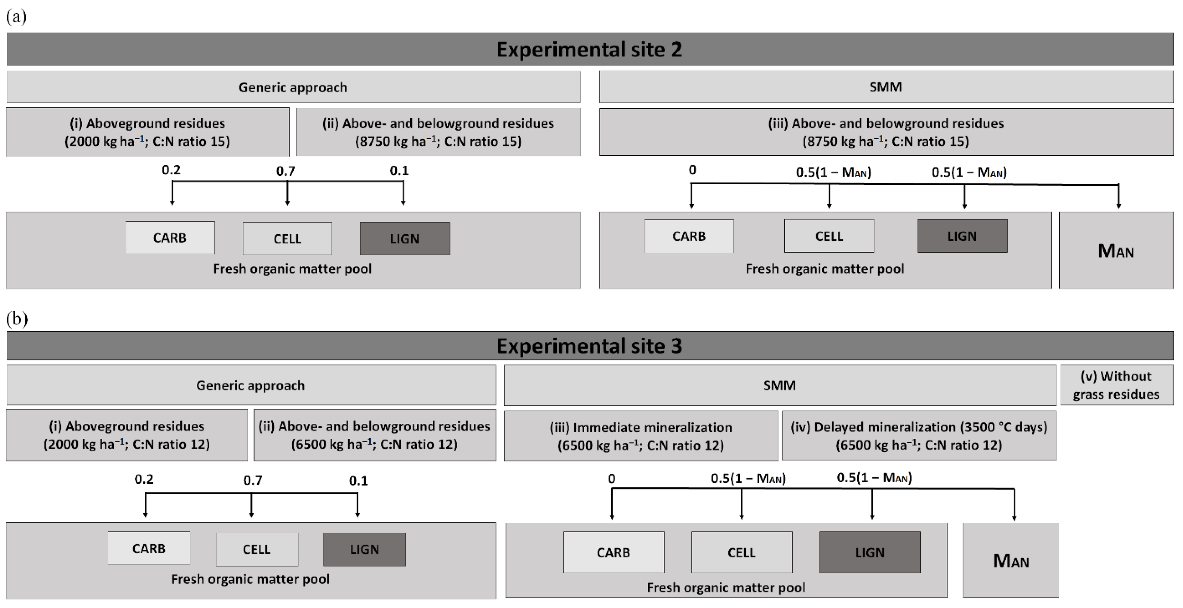
2.4. Model Adaptations to Predict Residual Nitrogen Effect

Ley termination and increased mineralization from plant residues and SOM accumulated in the previous years is currently not captured well in APSIM [17]. Therefore, model adjustments were made to identify potential options for improvement to predict the N release after a ley phase. For this purpose, the two experimental sites with a ley phase, i.e., E2 and E3, were used. Suitability of each of the alternative approaches for modeling the residual N effect of ley to the following maize crop was evaluated by comparing model outcomes and experimental data for biomass yield, N yield, and N leaching.

When using the manager script ‘Kill AgPasture’, the aboveground biomass is automatically removed from the system when AgPasture is terminated. Hence, we first tested if the N dynamics after termination of the ley phase could be simulated correctly when compensating only for this loss. This would be a practically easy way to compensate for the underestimation of mineralization occurring after a ley phase in APSIM. To do so, we added 2000 kg ha⁻¹ aboveground grass residues at the end of the ley phase. These grass residues were directly added to the FOM, with the default partitioning of 20% CARB, 70% CELL, and 10% LIGN using manager scripts, here termed as ‘generic approach accounting for aboveground residues (APSIM-G_a)’. This is denoted as modeling approach (i) in Figure 1a,b.

In addition, there is an underestimation of the large amount of belowground biomass produced over time when using the AgPasture model [17]. The default predicted belowground biomass was only ~500 kg DM ha⁻¹ for E2 and E3. The same default partitioning was used to compensate for both aboveground residues and additional root dry matter, here termed as ‘generic approach accounting for above- and belowground grass residues (APSIM-G_ab)’. We added 8750 kg ha⁻¹ to mimic additional aboveground residues and root dry matter at the end of the ley phase for E2, according to measurements from Acharya et al. [34]. Most residues were added to the upper soil (2000 kg ha⁻¹ aboveground residues and 2700 kg ha⁻¹ root dry matter in 0–28 cm). The remaining amount of root dry matter was 2700, 900, and 450 kg ha⁻¹ allocated at 28–35, 35–43, and 43–52 cm soil depth, respectively [11,34]. This is modeling approach (ii) in Figure 1a. The amount of root dry matter is dependent on the length of the ley phase [34]. In E3, the ley was grown for a shorter period compared with E2; therefore, in total, 6500 kg ha⁻¹ additional above- and belowground grass residues were added. This is modeling approach (ii) in Figure 1b.

As the fresh root dry matter is likely prone to immediate decomposition after the ley is ploughed, and the generic approach in APSIM might not capture this directly [17], we also tested a previously described model, which has been developed to improve model predictions for the mineralization of catch crop residues [35]. This simple mineralization model (APSIM-SMM) uses an additional conceptual OM pool (i.e., the M_AN fraction in Figure 1) to better reflect decomposition of fresh plant residues by faster mineralization.

The M_AN fraction is the maximum fraction of grass residue N that can be released over 200 days. The remaining is added to the CELL and the LIGN pools and decomposes slowly. Each day a fraction of the M_AN pool that mineralizes is computed and added as NH₄, in which the rate is dependent on the C:N ratio of the added residue, temperature, and soil moisture [35]. This is modeling approach (iii) in Figure 1a,b. In the measured data leaching increased in the second year after termination of the pure ryegrass ley was observed in E3. Therefore, in one of the modeling approaches, a delay of 3500 °C days (+/− 1 year) before mineralization of the residue starts was tested (iv), shown in Figure 1b. For E3, which only had one short period with ryegrass ley, APSIM was also run without a ryegrass period (v) in Figure 1b. The C:N ratio of the residues was set to 15 for E2 and 12 for E3 in all the modeling approaches, to ensure rapid mineralization of N in the period following ley as observed in field experiments [17,36].

2.5. Model Evaluation

Model outcomes were compared with experimental data using several statistical indexes (Equations (1)–(3)); these included the coefficient of determination (R²), the Nash-Sutcliffe efficiency score (NSE), the root mean square error (RMSE), and percentage bias (Pbias). The NSE score compares the predicted mean square error with the variance of the observations. A positive NSE indicates that the model has more predictive power than the mean observations [37]. The RMSE is an indication for the absolute error between the observed and simulated numbers. The RMSE values can extend from zero to infinity, but when they approach zero, the residual estimation error is decreased.

For Pbias the optimal value is 0, a negative value indicates that a model tends to underestimate the measured values, whereas a positive value indicates an overestimation [38].

$$\mathrm{RMSE}=\sqrt{\left[\left(\frac{1}{n}\right){\displaystyle \sum }_{i=1}^n{(S_i-O_i)}^2\right]}$$

(1)

$$\mathrm{NSE}=1-\frac{{{\displaystyle \sum }}_{i=1}^n{(S_i-O_i)}^2}{{{\displaystyle \sum }}_{i=1}^n{(S_i-\overline{O})}^2}$$

(2)

$$\mathrm{Pbias}=100\frac{{{\displaystyle \sum }}_{i=1}^n(S_i-O_i)}{{{\displaystyle \sum }}_{i=1}^n{O}_i}$$

(3)

where $S_i$, $O_i$ and $\overline{O}$ are the simulated, observed, and mean of the observed values, respectively, and n is the number of observations in the dataset. In this study, the model performance is discussed for maize biomass, maize N yield (E1, E2 and E3), and N leaching (E2 and E3). For E1, only the model outcomes regarding the phenology of maize and biomass of maize were evaluated, as no measurements of N leaching were done at this site.

3. Results

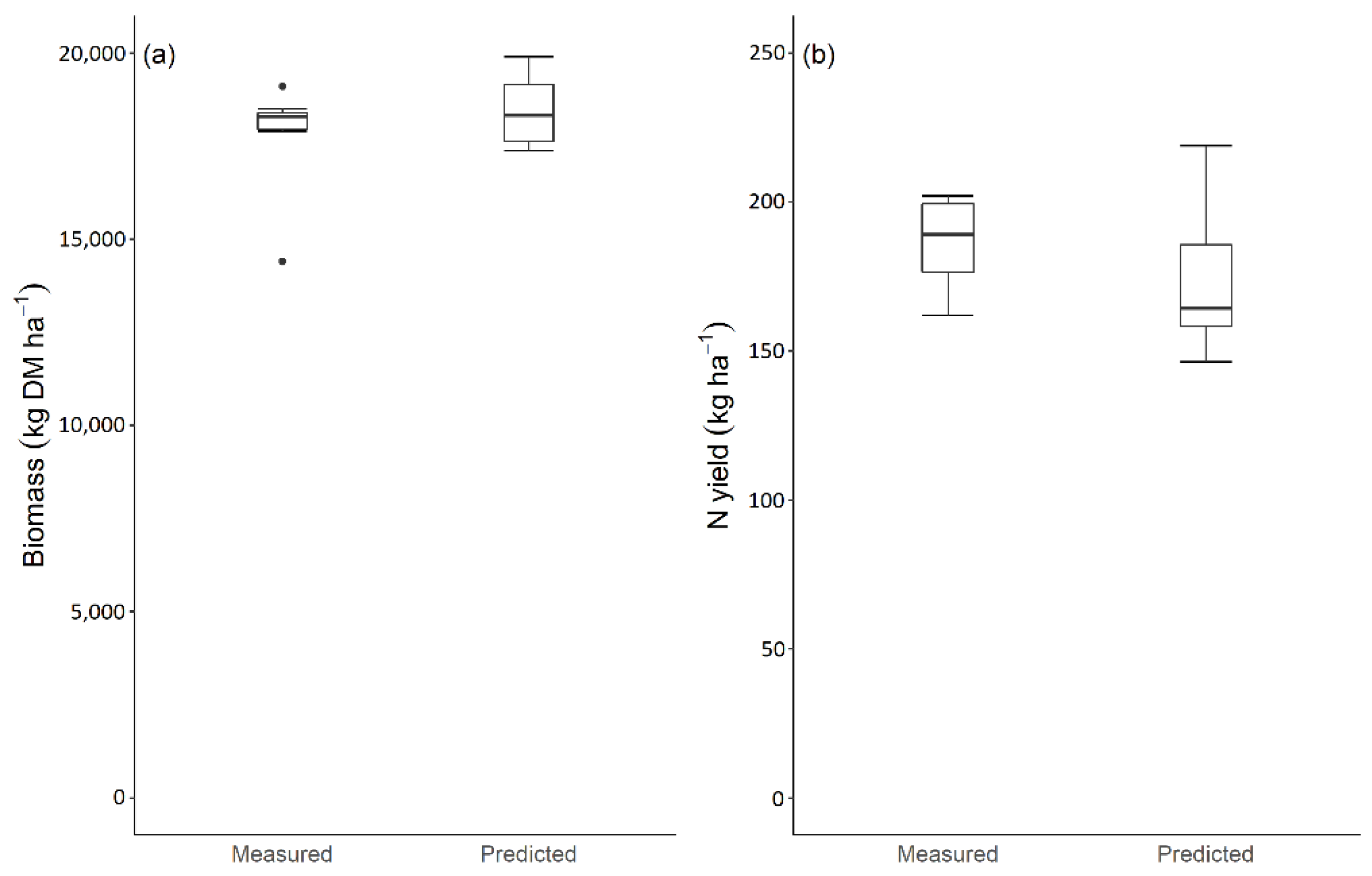
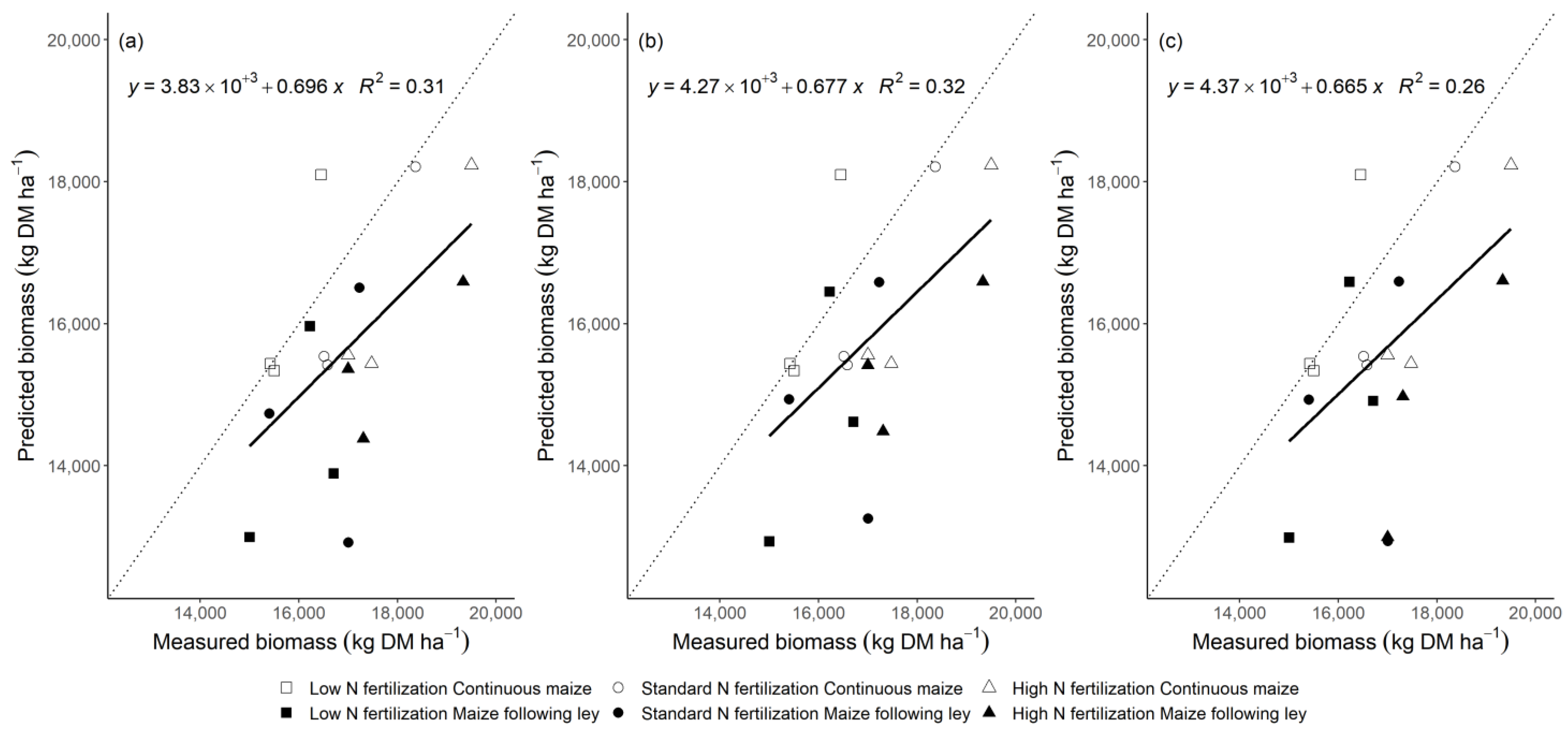
3.1. Model Performance to Predict Maize Biomass Yield

For E1, results were based on simulating maize production without a ley phase and no different modeling approaches for predicting the residual N were tested (

Table 3. Model performance statistics for dry matter (DM) and N yields of forage maize at experimental site 1 (n = 7); RMSE = root mean squared error (kg ha⁻¹ year⁻¹), NSE = Nash Sutcliffe efficiency score (−), and Pbias = percent bias (%).

	DM	N Yield
R2	0.16	0.04
RMSE	1506	38
NSE	−0.11	−1.95
Pbias	3.80	−7.50

, Figure 2a). The average of the measured biomass was 17,785 kg DM ha⁻¹, with a range from 14,417 up to 19,143 kg DM ha⁻¹. APSIM tended to slightly overestimate biomass yield; the largest overestimation was found for the relatively low biomass yield in 2014 (~14,400 kg DM ha⁻¹) being almost 3000 kg DM ha⁻¹ lower than predicted by APSIM (~17,400 kg DM ha⁻¹). With an RMSE of 1506 kg DM ha⁻¹, but a fairly low R² and a negative NSE model, the performance model performance is judged to be reasonable to poor.

For APSIM-G_a, APSIM tended on average to underestimate biomass production as indicated by the negative Pbias for E2 (

Table 4. Model performance statistics for forage maize dry matter (DM) (n = 18) and nitrogen (N) yield (n = 18) as well as N leaching (n = 18) for the continuous maize and maize following grass-clover ley at low, standard, and high N fertilization levels for experimental site 2; RMSE = root mean squared error (kg ha⁻¹ year⁻¹), NSE = Nash Sutcliffe efficiency score (−), and Pbias = percentage bias (%). Testing used the generic approach accounting for aboveground residues (2000 kg ha⁻¹ year⁻¹), above- and belowground residues (8750 kg ha⁻¹ year⁻¹), and the simple mineralization model (SMM; 8750 kg residues kg ha⁻¹ year⁻¹; see Figure 1).

	Generic Approach			Generic Approach			SMM
	Aboveground			Above- and Belowground
	DM	N Yield	N Leaching	DM	N Yield	N Leaching	DM	N Yield	N Leaching
RMSE	1846	30	113	1735	23	90	1920	27	37
NSE	−1.32	−0.18	−1.51	−1.05	0.30	−0.61	−1.51	0.09	0.72
Pbias	−7.70	−6.70	−59.40	−7.10	−2.50	−46.40	−7.60	4.70	−12.30

, Figure 3). For example, APSIM underpredicted biomass production in the maize following the ley system at the low and standard N fertilization rates in 2011. Besides, a RMSE of 1846 kg DM ha⁻¹ was found and a negative NSE was found for E2. In case of E3, however, the model tended to slightly overestimate the maize DM yield as indicated by the positive Pbias (

Table 5. Performance statistics for harvested maize dry matter (n = 6) for experimental site 3; R² = coefficient of determination, RMSE = root mean squared error (kg ha⁻¹ year⁻¹), NSE = Nash Sutcliffe efficiency score (−), and Pbias = percentage bias (%). Tested modeling included the generic approach accounting for aboveground residues (2000 kg ha⁻¹ year⁻¹), for above- and belowground residues (6500 kg ha⁻¹ year⁻¹), and the simple mineralization model (SMM) with immediate and delayed mineralization (6500 kg residues kg ha⁻¹ year⁻¹) and the approach without a ryegrass period (see Figure 1).

	Generic Approach	Generic Approach	SMM	SMM	Without a Ryegrass Period
	Aboveground	Above- and Belowground	Immediate Mineralization	Delayed Mineralization
R2	0.82	0.79	0.75	0.74	0.86
RMSE	1487	1666	1664	1680	1299
NSE	0.48	0.34	0.35	0.33	0.60
Pbias	7.90	9.50	8.90	8.90	6.60

). In addition, a RMSE of 1487 kg DM ha⁻¹ and a positive NSE were found for E3. The positive NSE shows that APSIM had more predictive power than using the mean of the observations.

For the APSIM-G_ab, the goodness-of-fit values slightly improved for E2 compared with APSIM-G_a (Table 4, Figure 3). Similar to APSIM-G_a, APSIM tended to underpredict biomass production. For E3, however, using this approach did not result in improved model predictions. For example, the RMSE increased from 1487 (APSIM-G_a) to 1666 (APSIM-G_ab) kg DM ha⁻¹ (Table 5).

For APSIM-SMM, model predictions did not improve compared with the two generic turnover approaches for E2 (Table 4, Figure 3). Using this modeling approach, APSIM also tended to underestimate biomass production. The RMSE increased, for example, with 74 and 185 kg DM ha⁻¹ compared with the APSIM-G_a and APSIM-G_ab, respectively. For E3, similar results were found for the SMM with immediate and delayed mineralization (Table 5). In addition, the results found using the SMM are comparable to those using two generic turnover approaches. The prediction accuracy was, however, best for the approach without a ryegrass period (Table 5).

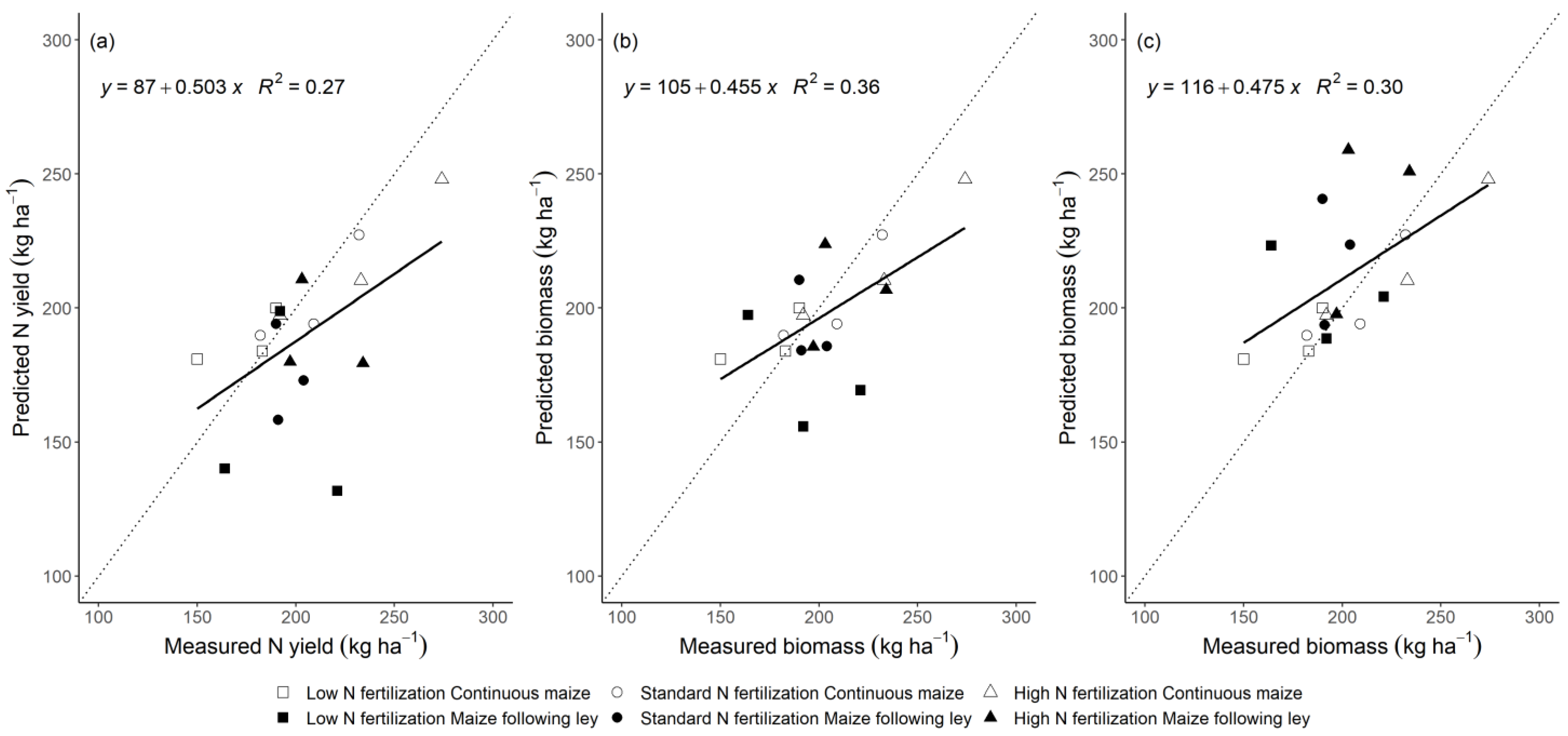
3.2. Model Performance to Predict Maize Nitrogen Yield

For E1, the negative Pbias shows that, on average, APSIM tended to underestimate the N yield. The largest deviation was found for the last two simulated years (2018 and 2019) for which measured values were underestimated with more than 50 kg N ha⁻¹. However, a large variation was found in the predicted values (146–219 kg N ha⁻¹) and for some years APSIM simulated a higher N uptake than measured, which eventually compensated the Pbias values. The RMSE was 38 kg N ha⁻¹, the low R² and negative NSE indicate a poor model performance.

For APSIM-G_a, a poor model fit was found for E2 (Table 4, Figure 4). The highest RMSE was found for this approach, the NSE was negative and N yield was tended to be underestimated. Additionally, for E3, the low R², the negative Pbias, and negative NSE indicate a poor model performance (

Table 6. Performance statistics of maize nitrogen yield (n = 6) for experimental site 3; R² = coefficient of determination, RMSE = root mean squared error (kg ha⁻¹ year⁻¹ ), NSE = Nash Sutcliffe efficiency score (−), and Pbias = percent bias (%) without a ryegrass period; tested using the generic approach accounting for aboveground residues (2000 kg ha⁻¹ year⁻¹), above- and belowground residues (6500 kg ha⁻¹ year⁻¹), and the simple mineralization model (SMM) with immediate and delayed mineralization (see Figure 1).

	Generic Approach	Generic Approach	SMM	SMM	Without a Ryegrass Period
	Aboveground	Above- and Belowground	Immediate Mineralization	Delayed Mineralization
R2	0.25	0.49	0.56	0.06	0.44
RMSE	37	29	27	43	35
NSE	−0.17	0.31	0.38	−0.53	−0.02
Pbias	−12.80	−5.00	−4.40	−11.30	−13.00

).

For APSIM-G_ab, a positive NSE was found for E2, pointing more predictive power of this modeling approach (Table 4). Moreover, values for R², RMSE and Pbias improved for this approach compared with APSIM-G_a (Table 4, Figure 4). For E3, model predictions improved as well, as indicated by the higher R², the RMSE of 29 kg N ha⁻¹, positive NSE, and lower Pbias.

For APSIM-SMM, the prediction accuracy was between the two generic turnover approaches for E2 (Table 4, Figure 4). The RMSE of 27 kg N ha⁻¹, positive NSE, and improved Pbias indicate a better model fit for APSIM-SMM compared with APSIM-G_a. Using the SMM, however, did not result in better prediction compared with APSIM-G_ab. Interestingly, the positive effect of the high N fertilization rates on N yield was lower compared to the measured data in the maize following the ley system for the generic approaches as well as for APSIM-SMM. Similarly, in the measured data, a decline of 33 kg N ha⁻¹ was found for the continuous maize system for the low compared to the standard fertilization rate, while in the model predictions this was only 15 kg N ha⁻¹. For E3, the best model fit was found for the SMM with immediate mineralization, where N yield was only slightly underpredicted and the NSE was positive (Table 6). Using the SMM with delayed mineralization did not improve model predictions compared with immediate mineralization. Furthermore, model accuracy was not better for the approach without a ryegrass period compared APSIM-G_a or the SMM with immediate mineralization.

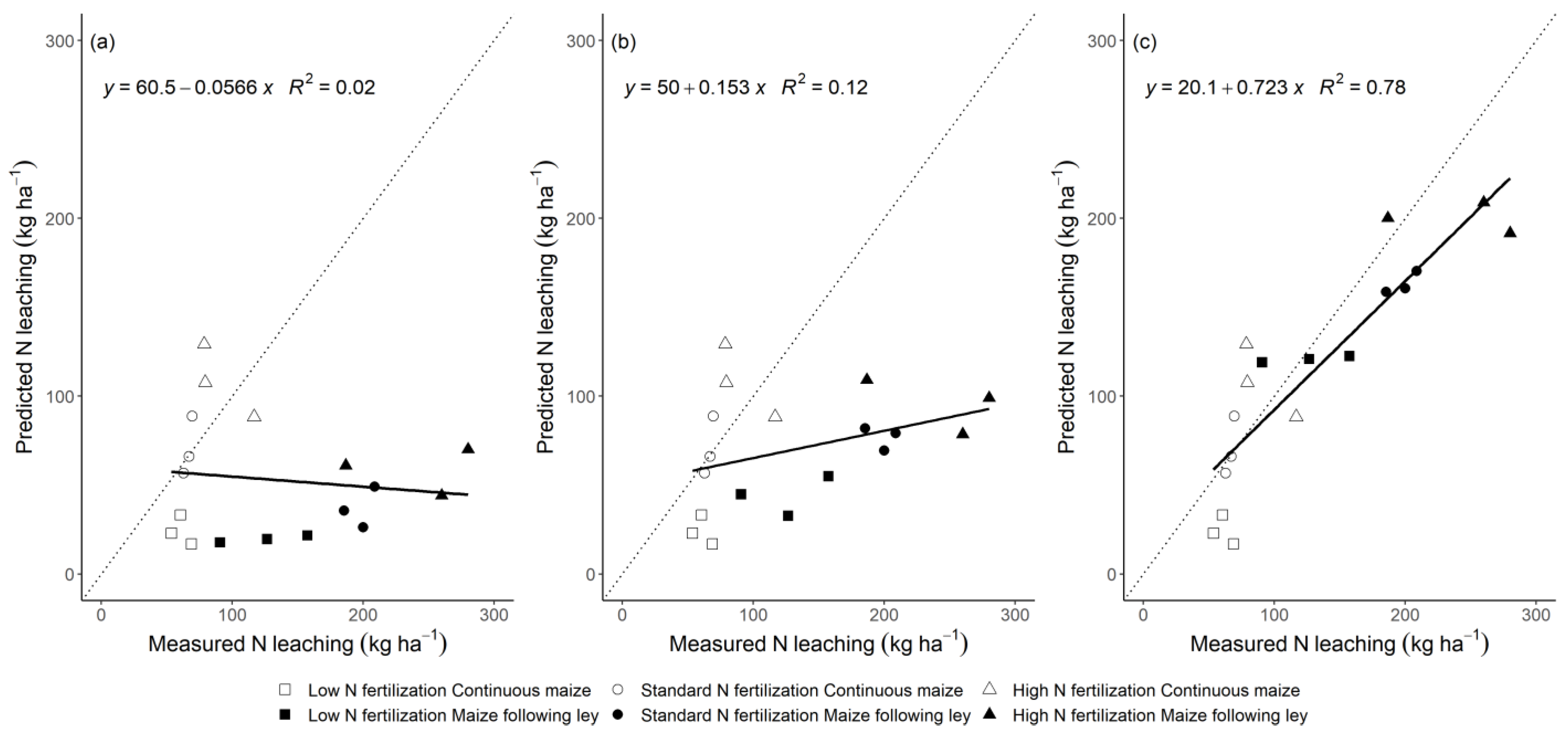
3.3. Model Performance to Predict Nitrogen Leaching

Model performance to predict N leaching was tested only for E2 and E3.

For APSIM-G_a, a large underprediction of N leaching was found for E2 (Table 4, Figure 5). Similarly, the results of other statistical indexes, including R², RMSE, and NSE, indicate a poor model performance. The maize following ley resulted in the highest N leaching levels and was strongly influenced by the fertilization rate, according to the measured data. For E3, a high negative Pbias was found for APSIM-G_a (

Table 7. Performance statistics for annual nitrogen leaching (n = 7) for experimental site 3; R² = coefficient of determination, RMSE = root mean squared error (kg ha⁻¹ year⁻¹ ), NSE = Nash Sutcliffe efficiency score (−), and Pbias = percentage bias (%). Tested modeling approaches included the approach without a ryegrass period, the generic approach accounting for aboveground residues (2000 kg ha⁻¹ year⁻¹), above- and belowground residues (6500 kg ha⁻¹ year⁻¹), and the simple mineralization model (SMM) with immediate and delayed mineralization (see Figure 1).

	Generic Approach	Generic Approach	SMM	SMM	Without a Ryegrass Period
	Aboveground	Above- and Belowground	Immediate Mineralization	Delayed Mineralization
R2	0.34	0.09	0.03	0.37	0.00
RMSE	21	24	26	21	25
NSE	0.08	−0.14	−0.38	0.13	−0.27
Pbias	−35.60	−21.80	−17.20	−33.80	−14.00

).

For APSIM-G_ab, model predictions improved for E2, as indicated by a higher R², a lower RMSE of 90 kg N ha⁻¹, and improved NSE and Pbias values compared with APSIM-G_a. In case of E3, however, using this approach did not result in an improved model performance. The NSE, for example, decreased from 0.08 to −0.14.

For APSIM-SMM, the prediction accuracy was best for E2 as indicated by a higher R² and a positive NSE compared with the two generic approaches (Table 4, Figure 5). Furthermore, the lowest RMSE was obtained, and N leaching was less underpredicted using the SMM. In contrast, using the SMM for E3 did not result in a clear improvement of model predications (Table 7). The R², RMSE, and NSE were, however, better for the approach with delayed compared with immediate mineralization. Using the delayed mineralization in the SMM resulted, however, in an increased underprediction as indicated by the high negative Pbias.

Figure 6 shows the cumulative N leaching over the full observation period for E3. When APSIM was run without a ryegrass period, the predicted cumulative N leaching (275 kg N ha⁻¹) was closest to the measured data (315 kg N ha⁻¹). During the winter of 2015–2016, one year after the ley period, when no cover crops were grown, a peak of N leaching was observed. Both the SMM with immediate mineralization and the generic approach accounting for above- and belowground residues, predicted a peak in N leaching, but in the winter period the year before. A similar cumulative leaching pattern was found for the generic approach accounting for aboveground residues and the SMM model with delayed mineralization. These two approaches predicted only a small peak in the winter period in the same year the ley was ploughed in, after which it gradually increased.

4. Discussion

4.1. Overall Model Performance of APSIM to Simulate Biomass Yield, N Yield, and N Leaching in Maize Systems in Northwest Europe

Earlier studies have reported that process-based models often have difficulties to predict crop yields and N dynamics in crop rotations with a high accuracy under a wide range of conditions [17,38,39,40,41,42]. Manevski et al. [23], for example, found a R² of 0.69 for maize DM and maize N content validating the process-based model DAISY, when using data of a maize monocrop system in Denmark. Results were found to be less accurate when an intercropped maize system was simulated compared to the monocrop system. In case of the intercropped system, a R² of −0.12 was reported for maize DM and −0.21 for N content. The model fit for N leaching was, however, good, with a R² of 0.83. Using DSSAT-CERES-Maize, another simulation model being used for an experiment in Canada, to simulate yield and N dynamics for a long-term continuous maize production system did not result in accurate predictions of annual maize yields, with a R² of 0.36 and 0.40, dependent on the fertilization level. Furthermore, a negative model efficiency was found, which indicates that the simulated values were worse than simply using mean values. It was concluded that the model simulated N leaching reasonably well as both a positive (0.64) and negative model efficiency (−8.0) were found [43]. Similarly, APSIM also has difficulties to capture the full complexity and dynamics of factors affecting crop production [44,45]. Here we explored if the APSIM Maize model could be used to predict biomass yield, N yield, and N leaching across different regions and forage maize systems in northwest Europe.

The results collectively suggested that the model performance of APSIM in its current state was poor to reasonable for estimating maize biomass, maize N yield, and N leaching across the different systems and experimental sites included in this study. The low R² and negative NSE that were frequently observed in this study could, however, be caused by the narrow range of measured values. Especially for E1 and E3, no replicates or different fertilization levels were available. Interpreting results of a statistical evaluation with only a limited amount of observations is difficult, and ideally, separate datasets would have been used for independent model calibration and validation [46]. In addition, some of the measurements did not reflect the expected responses to N fertilization in E2.

A second factor that could have influenced model performance is the amount of crop variables used to assess model performance. In this study, we only considered two crop variables; thus, the observed over- or underprediction could be caused by a cascading effect of other crop variables. An overestimation of maize leaf number, for example, can finally result in a too high predicted biomass production and total N uptake [47]. Flowering is, however, one of the key components for accurate simulation of phenological development [48]. In APSIM, this is based on a specific thermal time target, and data of E1 could be used in this study. As highlighted by Akhavizadegan et al. [49], the estimation of parameters, such as cultivar or soil input values, is a time-consuming and challenging procedure that is susceptible to errors. Even models with a similar structure can, for example, give very different model fits to the same dataset, depending on the model users and their calibration protocol [46,50].

A third potential factor contributing to the uncertainty in model predictions are the mathematical functions used to simulate temperature responses of physiological processes [51]. Since the mean air temperatures were different across the three study sites, and one function was fitted to simulate this relation, this could have influenced the simulated phenological development and predicted biomass.

Another factor is the uncertainty related to N leaching predictions, which is more frequently observed in modeling studies [52]. This has been attributed to a time offset between simulated and measured leaching, spatial variability in soil hydraulic properties within a field, the often high uncertainty in N leaching measurements, and the general complexity of soil N dynamics [22,42]. For example, limitations of using suction cups for N leaching measurements include the uncertainty in the sampling volume and the influence on natural soil water flows [53].

To conclude, although the overall model performance was judged to be reasonable to poor, several factors might have influenced the results. While the use of data from different experimental sites could potentially contribute to improving the testing power and robustness of APSIM, it also has its limitations. In this study, using datasets from different experimental sites without common protocol structurally limited the accuracy figures for biomass, maize N yield, and N leaching. Nevertheless, APSIM has proven to be an interesting tool for modeling, based on biological processes and generalization for northwest Europe. Using more datasets in combination with a framework to capturing historical yield trends and combining simulation results from multiple models are interesting steps to improve model predictions and to facilitate long-term simulations [38,49]. Furthermore, to reduce the uncertainty related to input parameters, the use of long-term datasets with detailed knowledge about methodologies facilitates the option to use a spin-up period. The initial size of the SOM pools is then, for example, better reflected [47,54]. Finally, the model performance can be improved by adaptations of various model components in APSIM. In this study, we specifically focused on model adaptations to predict the residual N effect, which is outlined in the next sections.

4.2. Belowground Biomass and Residual Nitrogen Effect of Ley Pastures

The results point to caution when using the current AgPasture and SoilN models for modeling ley-arable systems, and imply on need to improve these models for this purpose. Specifically, modifications are needed to better reflect the development of belowground biomass and the subsequent decomposition of OM when the grassland ley is ploughed. Previous studies often only used AgPasture in a permanent grassland system with a focus on aboveground biomass production and composition of the grassland ley, as well as N leaching in grazing systems [55,56,57].

Root biomass and SOM increase with ley age until an equilibrium is reached [12]. In field experiments, it was shown that the development of root biomass after cropland conversion to grassland is progressive with 30% and 80% after 12 and 24 months, respectively [58].

Therefore, we assumed that the quantity of the extra residues needed to be added in APSIM was lower in E3 than in E2. The amounts for both sites were relatively high compared to the 7000 kg ha⁻¹ additional biomass used by Hoffmann et al. [17] after the break-up of a permanent grassland. The quantities assumed in this study are, however, subjected to uncertainty because the amount of plant residues was not always found to be related to ley age, and a wide range of root biomass in temperate grasslands has been reported [11,15,16]. In addition, information regarding the amount and composition of belowground biomass is subject to a high variability due to methods employed to separate roots from soil and conditions under which the measurements have been obtained [59,60]. Despite these uncertainties, the findings of this study suggest that modifications are needed in the AgPasture model, such as the root turnover rate, the senescence of roots, and the root-to-shoot ratio to better account for belowground biomass production. Chen et al. [61] showed that the belowground net primary production could be well predicted by a linear regression using grass shoot measurements. This might be a potential way to improve model predictions.

Modeling soil N dynamics and N leaching after the break-up of the ley is another challenge where models often tend to have difficulties. The residual effect is of particular interest for ley-arable systems and its effect on N mineralization can be substantial [13,36]. The N accumulation and release are influenced by many factors and interacting processes such as climate conditions, ley management and composition, age, and soil type [62,63]. The mineralization of OM after a ley phase has been described as a two-stage process, with an initial phase of rapid mineralization over the first 160–230 days, followed by a second phase in which mineralization rates decrease progressively and are two to seven times lower compared to the initial phase [12,36,64]. The high amounts of residual N after a ley make this a particular period, prone to leaching losses. Measurements at E2 showed that even at low N fertilization levels, N leaching is substantially higher in the maize following ley (91–157 kg N ha⁻¹ year⁻¹) compared with the continuous maize (54–69 kg N ha⁻¹ year⁻¹). The effect of ley ploughing on N dynamics in the following years is unknown at this site. In contrast to what would be expected, measurements did not show the expected rapid N mineralization and peak in N leaching in the first year after termination of the ley phase at E3.

Reducing fertilization levels in the first growing season after a ley up to a rate of 0 kg N ha⁻¹ and the use of cover crops are efficient strategies to mitigate N leaching [62,64]. Both the measurements and model predictions showed a decline in N leaching when the low N fertilization levels were used for E2. Even during the second year the effect on N dynamics can still be noticeable, in combination with the N conserved in the catch crop over the winter [64]. Thus, additional N fertilization induces a risk that N availability exceeds crop demand as observed by Kayser et al. [62]. In contrast, the ley period is characterized by a sharp reduction in N leaching to groundwater [65]. Therefore, to be able to compare the environmental impact of continuous cropping systems with ley-arable systems, full cropping cycles need to be considered.

4.3. Comparison of the Generic and the Modified Approach

We hypothesized that the generic approach in APSIM would not be able to accurately describe the amount and timing of N cycling from ley to arable systems. Here, we tested three different modeling approaches to improve the model performance of APSIM by simulating the residual N effect of ley to the following crop more accurately.

The results indicated that predictions of maize biomass yield did improve with APSIM-G_ab, while using APSIM-SMM was not of added value for E2. In case of E3, however, the approach without a ryegrass period resulted in the highest accuracy. This could be related to the limited number of measurements to validate model performance, and the limited effect of increased N availability on maize biomass production.

N yield predictions improved with APSIM-SMM compared with APSIM-G_a. The APSIM-G_ab, however, had the highest accuracy for N yield among the three modeling approaches for E2. Similar to E2, model predictions improved when accounting for belowground grass residues for E3. The best model fit was found for the SMM with immediate mineralization. Overall, this shows the sensitivity of model predictions to both the amount of available N and to the timing of mineralization of grass residues.

In contrast to maize biomass yield and N yield predictions, the SMM resulted in the highest accuracy for N leaching for E2. This shows that enhancing mineralization with SMM was an effective strategy to improve model predictions compared with the generic approach. For the two generic approaches, the unsatisfactory model fit for N leaching is caused by the slower mineralization of grass residues. Hence, the relatively high measured N leaching was not simulated in the first maize year after termination of the ley phase. The results of E3 showed the difficulty of finding an appropriate set up even when only three model outputs were considered. None of the approaches outperformed the others for forage maize biomass, N yield, and leaching across all the statistical indexes. For E3, the observed rapid increase in N leaching in winter 2015–2016 might be attributed to the bare soil during that period. The surplus of N was not retained in the system and easily drained out of the root zone.

Despite inconclusive results for the three studied parameters across the different modeling approaches and sites, we speculated that the results of E2 might be more reliable due to the use of replicates and different N fertilization rates. Nevertheless, we concluded that accounting for belowground residues seems especially important for N yield predictions, but less for harvestable forage maize biomass. Our study clearly documented and added value of the SMM to improve N mineralization patterns and N leaching after a ley phase in APSIM. Potential limitations of the alternative modeling approaches used in this study are outlined below.

Previous studies have demonstrated that, in specific cases, the decomposition of plant residues is underestimated when FOM pools and turnover rates are based on default values. Adjustments were, therefore, made in the partitioning of residues to the different FOM pools by better accounting for the biochemical composition and increasing FOM pool sizes [27,35,66,67]. The SMM used here is based on incubation studies of Brassica catch crop residues with a C:N ratio lower than 25. The derived model parameters of these incubations studies might not necessarily fully align with the mineralization pattern of grass residues [68]. In this study, we used relatively low C:N ratios, and the use of static values might not correctly reflect the related C dynamics [35].

The C:N ratio of residues was set to 15 for E2 and 12 for E3 to ensure timely mineralization in APSIM and to find a balance between simulated biomass, N yield, and N leaching for each site. Both figures are in line with data gathered from literature under high N input levels [68]. The measured C:N ratios of grassland residues can, however, cover a wide range. Vertès et al. [12] documented for both pure ryegrass and grass-clover residues values between 14 and 33. This variability is caused by, for example, the species composition of the ley, their phenology at harvest, and the type and quantity of fertilizer applied [34].

The use of field datasets from ley-arable systems is useful to assess APSIM’s suitability for simulating the N dynamics that occur in these systems. With the addition of extra grass residues, we were able to reproduce, i.e., mimic the increased mineralization typically occurring after termination of the ley. Ideally, data of long-term ley-arable experiments with various ley lengths, fertilization levels, and different species compositions should be used in further studies to fully reveal the robust approach for modeling these systems in APSIM. In addition, analyzing the implementation of leys at higher spatial scales, for example, within regionally integrated crop–livestock systems, is a prerequisite to assess its full potential in sustainable future food systems.

5. Conclusions

We evaluated the robustness of APSIM to predict biomass yield, N yield, and N leaching of different forage maize systems in northwest Europe, while using different approaches to predict the residual N effect. The model simulated biomass and N yield of maize fairly well across the different systems and sites, independent of using the generic approach or the SMM. When APSIM was linked with the SMM, the prediction accuracy of N leaching improved at E2, regardless of the fertilization level. This clearly documents an inherent shortcoming of APSIM to capture enhanced mineralization in arable crops following ley cultivation. In all the modeling approaches, APSIM had difficulties to predict a delay of N leaching after a ley observed at E3. Therefore, we conclude that APSIM requires a process description review related to OM mineralization in ley-arable systems, at least under the pedo-climatic conditions in northwest Europe. Accounting for belowground residues of leys seems to be important for N yield predictions of the following crop, while the SMM could be of added value to improve the predication of the mineralization patterns and N leaching after a ley phase in APSIM. A comprehensive modeling approach is, therefore, needed to predict the N transfer to the following crops in APSIM. This is of particular interest for ley-arable systems due to the large input of OM.

References

1. De Boer, I.J.M.; van Ittersum, M.K. Circularity in Agricultural Production; Wageningen University & Research: Wageningen, The Netherlands, 2018; pp. 1–74. [Google Scholar]
2. Velthof, G.L.; Lesschen, J.P.; Webb, J.; Pietrzak, S.; Miatkowski, Z.; Pinto, M.; Kros, J.; Oenema, O. Science of the Total Environment The impact of the Nitrates Directive on nitrogen emissions from agriculture in the EU-27 during 2000–2008. Sci. Total Environ. 2014, 468–469, 1225–1233. [Google Scholar] [CrossRef] [PubMed]
3. Wachendorf, M.; Buchter, M.; Trott, H.; Taube, F. Performance and environmental effects of forage production on sandy soils. II. Impact of defoliation system and nitrogen input on nitrate leaching losses. Grass Forage Sci. 2004, 59, 56–68. [Google Scholar] [CrossRef]
4. Abalos, D.; van Groenigen, J.W.; Philippot, L.; Lubbers, I.M.; De Deyn, G.B. Plant trait-based approaches to improve nitrogen cycling in agroecosystems. J. Appl. Ecol. 2019, 56, 2454–2466. [Google Scholar] [CrossRef]
5. Lemaire, G.; Franzluebbers, A.; de Faccio Carvalho, P.C.; Dedieu, B. Integrated crop-livestock systems: Strategies to achieve synergy between agricultural production and environmental quality. Agric. Ecosyst. Environ. 2014, 190, 4–8. [Google Scholar] [CrossRef]
6. Biernat, L.; Taube, F.; Vogeler, I.; Reinsch, T.; Kluß, C.; Loges, R. Is organic agriculture in line with the EU-Nitrate directive? On-farm nitrate leaching from organic and conventional arable crop rotations. Agric. Ecosyst. Environ. 2020, 298, 106964. [Google Scholar] [CrossRef]
7. Guillaume, M.; Durand, J.; Duru, M.; Gastal, F.; Julier, B.; Litrico, I.; Louarn, G.; Médiène, S.; Moreau, D.; Valentin-morison, M.; et al. Role of ley pastures in tomorrow’s cropping systems. A review. Agron. Sustain. Dev. 2020, 40, 17. [Google Scholar] [CrossRef]
8. Crème, A.; Rumpel, C.; Le Roux, X.; Romian, A.; Lan, T.; Chabbi, A. Ley grassland under temperate climate had a legacy effect on soil organic matter quantity, biogeochemical signature and microbial activities. Soil Biol. Biochem. 2018, 122, 203–210. [Google Scholar] [CrossRef]
9. van Eekeren, N.; Bommelé, L.; Bloem, J.; Schouten, T.; Rutgers, M.; de Goede, R.; Reheul, D.; Brussaard, L. Soil biological quality after 36 years of ley-arable cropping, permanent grassland and permanent arable cropping. Appl. Soil Ecol. 2008, 40, 432–446. [Google Scholar] [CrossRef] [Green Version]
10. Soussana, J.F.; Lemaire, G. Coupling carbon and nitrogen cycles for environmentally sustainable intensification of grasslands and crop-livestock systems. Agric. Ecosyst. Environ. 2014, 190, 9–17. [Google Scholar] [CrossRef]
11. Christensen, B.T.; Rasmussen, J.; Eriksen, J.; Hansen, E.M. Soil carbon storage and yields of spring barley following grass leys of different age. Eur. J. Agron. 2009, 31, 29–35. [Google Scholar] [CrossRef]
12. Vertès, F.; Hatch, D.; Velthof, G.; Taube, F.; Laurent, F.; Loiseau, P.; Recous, S. Short-Term and Cumulative Effects of Grassland Cultivation on Nitrogen and Carbon Cycling in Ley-Arable Rotations. Grassl. Sci. Eur. 2007, 12, 227–246. [Google Scholar]
13. Nevens, F.; Reheul, D. The nitrogen- and non-nitrogen-contribution effect of ploughed grass leys on the following arable forage crops: Determination and optimum use. Eur. J. Agron. 2002, 16, 57–74. [Google Scholar] [CrossRef]
14. Loges, R.; Bunne, I.; Reinsch, T.; Malisch, C.; Kluß, C.; Herrmann, A.; Taube, F. Forage production in rotational systems generates similar yields compared to maize monocultures but improves soil carbon stocks. Eur. J. Agron. 2018, 97, 11–19. [Google Scholar] [CrossRef]
15. Deru, J.; Schilder, H.; van der Schoot, J.R.; van Eekeren, N. Genetic differences in root mass of Lolium perenne varieties under field conditions. Euphytica 2014, 199, 223–232. [Google Scholar] [CrossRef] [Green Version]
16. Iepema, G.L.; Deru, J.G.C.; Hoekstra, N.J.; Van Eekeren, N.; Höglind, M.; Bakken, A.K.; Hovstad, K.A.; Kallioniemi, E.; Riley, H.; Steinshamn, H.; et al. Rooting of permanent grassland in relation to build-up of soil organic matter for climate mitigation. In The Multiple Roles of Grassland in the European Bioeconomy, Proceedings of the 26th General Meeting of the European Grassland Federation, Trondheim, Norway, 4–8 September 2016; Höglind, M., Bakken, A.K., Hovstad, K.A., Kallioniemi, E., Riley, H., Steinshamn, H., Østrem, L., Eds.; NIBIO, The Norwegian Institute of Bioeconomy Research: Trondheim, Norway, 2016; pp. 777–779. [Google Scholar]
17. Hoffmann, M.P.; Isselstein, J.; Rötter, R.P.; Kayser, M. Agriculture, Ecosystems and Environment Nitrogen management in crop rotations after the break-up of grassland: Insights from modelling. Agric. Ecosyst. Environ. 2018, 259, 28–44. [Google Scholar] [CrossRef]
18. Watson, C.A.; Baddeley, J.A.; Edwards, A.C.; Rees, R.M.; Walker, R.L.; Topp, C.F.E. Influence of ley duration on the yield and quality of the subsequent cereal crop (spring oats) in an organically managed long-term crop rotation experiment. Org. Agric. 2011, 1, 147–159. [Google Scholar] [CrossRef]
19. Holzworth, D.P.; Huth, N.I.; DeVoil, P.G.; Zurcher, E.J.; Herrmann, N.I.; McLean, G.; Chenu, K.; van Oosterom, E.J.; Snow, V.; Murphy, C.; et al. APSIM—Evolution towards a new generation of agricultural systems simulation. Environ. Model. Softw. 2014, 62, 327–350. [Google Scholar] [CrossRef]
20. Moeller, C.; Pala, M.; Manschadi, A.M.; Meinke, H.; Sauerborn, J. Assessing the sustainability of wheat-based cropping systems using APSIM: Model parameterisation and evaluation. Aust. J. Agric. Res. 2007, 58, 75–86. [Google Scholar] [CrossRef]
21. Böldt, M.; Taube, F.; Vogeler, I.; Reinsch, T.; Kluß, C.; Loges, R. Evaluating Different Catch Crop Strategies for Closing the Nitrogen Cycle in Cropping Systems—Field Experiments and Modelling. Sustainability 2021, 13, 394. [Google Scholar] [CrossRef]
22. Vogeler, I.; Kaag, I.; Friedhelm, T.; Poulsen, V.; Loges, R.; Møller, E. Effect of winter cereal sowing time on yield and nitrogen leaching based on experiments and modelling. Soil Use Manag. 2021, 38, 663–675. [Google Scholar] [CrossRef]
23. Manevski, K.; Børgesen, C.D.; Andersen, M.N.; Kristensen, I.S. Reduced nitrogen leaching by intercropping maize with red fescue on sandy soils in North Europe: A combined field and modeling study. Plant Soil 2015, 388, 67–85. [Google Scholar] [CrossRef]
24. Hammer, G.L.; Kropff, M.J.; Sinclair, T.R.; Porter, J.R. Future contributions of crop modelling from heuristics and supporting decision making to understanding genetic regulation and aiding crop improvement. Eur. J. Agron. 2002, 18, 15–31. [Google Scholar] [CrossRef]
25. Soufizadeh, S.; Munaro, E.; Mclean, G.; Massignam, A.; Van Oosterom, E.J.; Chapman, S.C.; Messina, C.; Cooper, M.; Hammer, G.I. Modelling the nitrogen dynamics of maize crops—Enhancing the APSIM maize model. Eur. J. Agron. 2018, 100, 118–131. [Google Scholar] [CrossRef]
26. Schrama, M.; De Haan, J.J.; Kroonen, M.; Verstegen, H.; Putten, W.H. Van Der Crop yield gap and stability in organic and conventional farming systems. Agric. Ecosyst. Environ. 2018, 256, 123–130. [Google Scholar] [CrossRef]
27. Keating, B.A.; Carberry, P.S.; Hammer, G.L.; Probert, M.E.; Robertson, M.J.; Holzworth, D.; Huth, N.I.; Hargreaves, J.N.G.; Meinke, H.; Hochman, Z.; et al. An overview of APSIM, a model designed for farming systems simulation. Eur. J. Agron. 2003, 18, 267–288. [Google Scholar] [CrossRef] [Green Version]
28. Probert, M.E.; Dimes, J.P.; Keating, B.A.; Dalal, R.C.; Strong, W.M. APSIM’s Water and Nitrogen Modules and Simulation of the Dynamics of Water and Nitrogen in Fallow Systems. Agric. Syst. 1998, 56, 1–28. [Google Scholar] [CrossRef]
29. Snow, V.; Huth, N. The APSIM-Micromet Module; HortResearch Internal Report No. 2004/12848; HortResearch: Palmerston North, New Zealand, 2004. [Google Scholar]
30. Foley, J.; Fainges, J. Soil Evaporation: How Much Water Is Lost from Northern Crop Systems and Do Agronomic Models Accurately Represent This Loss? 2014. Available online: https://grdc.com.au/resources-and-publications/grdc-update-papers (accessed on 16 March 2022).
31. Dalgliesh, N.; Hochman, Z.; Huth, N.; Holzworth, D. A Protocol for the Development of APSoil Parameter Values for Use in APSIM; Version 4; CSIRO: Canberra, Australia, 2016. [Google Scholar]
32. Ellermann, T.; Nygaard, J.; Christensen, J.H.; Løfstrøm, P.; Geels, C.; Nielsen, I.E.; Poulsen, M.B.; Monies, C.; Gyldenkærne, S.; Brandt, J.; et al. Nitrogen Deposition on Danish Nature. Atmosphere 2018, 9, 447. [Google Scholar] [CrossRef] [Green Version]
33. Moore, A.D.; Holzworth, D.P.; Herrmann, N.I.; Brown, H.E.; De Voil, P.G.; Snow, V.O.; Zurcher, E.J.; Huth, N.I. Environmental Modelling & Software Modelling the manager: Representing rule-based management in farming systems simulation models. Environ. Model. Softw. 2014, 62, 399–410. [Google Scholar] [CrossRef]
34. Acharya, B.S.; Rasmussen, J.; Eriksen, J. Grassland carbon sequestration and emissions following cultivation in a mixed crop rotation. Agric. Ecosyst. Environ. 2012, 153, 33–39. [Google Scholar] [CrossRef] [Green Version]
35. Vogeler, I.; Cichota, R.; Thomsen, I.K.; Bruun, S.; Jensen, L.S.; Pullens, J.W.M. Estimating nitrogen release from Brassicacatch crop residues—Comparison of different approaches within the APSIM model. Soil Tillage Res. 2019, 195, 104358. [Google Scholar] [CrossRef]
36. Hansen, J.P.; Eriksen, J.; Jensen, L.S. Residual nitrogen effect of a dairy crop rotation as influenced by grass-clover ley management, manure type and age. Soil Use Manag. 2005, 21, 278–286. [Google Scholar] [CrossRef]
37. Moriasi, D.N.; Arnold, J.G.; Van Liew, M.W.; Bingner, R.L.; Harmel, R.D.; Veith, T.L. Model Evaluation Guidelines for Systematic Quantification of Accuracy in Watershed Simulations. Trans. ASABE 2007, 50, 885–900. [Google Scholar] [CrossRef]
38. Kollas, C.; Kersebaum, K.C.; Nendel, C.; Manevski, K.; Müller, C.; Palosuo, T.; Armas-Herrera, C.M.; Beaudoin, N.; Bindi, M.; Charfeddine, M.; et al. Crop rotation modelling-A European model intercomparison. Eur. J. Agron. 2015, 70, 98–111. [Google Scholar] [CrossRef]
39. Salo, T.J.; Palosuo, T.; Kersebaum, K.C.; Nendel, C.; Angulo, C.; Ewert, F.; Bindi, M.; Calanca, P.; Klein, T.; Moriondo, M.; et al. Comparing the performance of 11 crop simulation models in predicting yield response to nitrogen fertilization. J. Agric. Sci. 2016, 154, 1218–1240. [Google Scholar] [CrossRef] [Green Version]
40. Yin, X.; Kersebaum, K.C.; Kollas, C.; Baby, S.; Beaudoin, N.; Manevski, K.; Palosuo, T.; Nendel, C.; Wu, L.; Hoffmann, M.; et al. Multi-model uncertainty analysis in predicting grain N for crop rotations in Europe. Eur. J. Agron. 2017, 84, 152–165. [Google Scholar] [CrossRef]
41. Yin, X.; Kersebaum, K.C.; Kollas, C.; Manevski, K.; Baby, S.; Beaudoin, N.; Öztürk, I.; Gaiser, T.; Wu, L.; Hoffmann, M.; et al. Performance of process-based models for simulation of grain N in crop rotations across Europe. Agric. Syst. 2017, 154, 63–77. [Google Scholar] [CrossRef]
42. Wolf, J.; Broeke, M.J.D.H.; Ro, R. Simulation of nitrogen leaching in sandy soils in The Netherlands with the ANIMO model and the integrated modelling system STONE. Agric. Ecosyst. Environ. 2005, 105, 523–540. [Google Scholar] [CrossRef]
43. Liu, H.L.; Yang, J.Y.; Drury, C.F.; Reynolds, W.D.; Tan, C.S.; Bai, Y.L.; He, P.; Jin, J.; Hoogenboom, G. Using the DSSAT-CERES-Maize model to simulate crop yield and nitrogen cycling in fields under long-term continuous maize production. Nutr. Cycl. Agroecosystems 2011, 89, 313–328. [Google Scholar] [CrossRef]
44. Peake, A.S.; Huth, N.I.; Carberry, P.S.; Raine, S.R.; Smith, R.J. Quantifying potential yield and lodging-related yield gaps for irrigated spring wheat in sub-tropical Australia. Field Crops Res. 2014, 158, 1–14. [Google Scholar] [CrossRef]
45. Yang, X.; Zheng, L.; Yang, Q.; Wang, Z.; Cui, S.; Shen, Y. Modelling the effects of conservation tillage on crop water productivity, soil water dynamics and evapotranspiration of a maize-winter wheat-soybean rotation system on the Loess Plateau of China using APSIM. Agric. Syst. 2018, 166, 111–123. [Google Scholar] [CrossRef]
46. Wallach, D.; Palosuo, T.; Thorburn, P.; Hochman, Z.; Andrianasolo, F.; Asseng, S.; Basso, B.; Buis, S.; Crout, N.; Dumont, B.; et al. Multi-model evaluation of phenology prediction for wheat in Australia. Agric. For. Meteorol. 2021, 298–299, 108289. [Google Scholar] [CrossRef]
47. Archontoulis, S.V.; Castellano, M.J.; Licht, M.A.; Nichols, V.; Baum, M.; Huber, I.; Martinez-Feria, R.; Puntel, L.; Ordóñez, R.A.; Iqbal, J.; et al. Predicting crop yields and soil-plant nitrogen dynamics in the US Corn Belt. Crop Sci. 2020, 60, 721–738. [Google Scholar] [CrossRef] [Green Version]
48. Parent, B.; Leclere, M.; Lacube, S.; Semenov, M.A.; Welcker, C.; Martre, P.; Tardieu, F. Maize yields over Europe may increase in spite of climate change, with an appropriate use of the genetic variability of flowering time. Proc. Natl. Acad. Sci. USA 2018, 115, 10642–10647. [Google Scholar] [CrossRef] [PubMed] [Green Version]
49. Akhavizadegan, F.; Ansarifar, J.; Wang, L.; Huber, I.; Archontoulis, S.V. A time-dependent parameter estimation framework for crop modeling. Sci. Rep. 2021, 11, 11437. [Google Scholar] [CrossRef]
50. Wallach, D.; Palosuo, T.; Thorburn, P.; Hochman, Z.; Gourdain, E.; Andrianasolo, F.; Asseng, S.; Basso, B.; Buis, S.; Crout, N.; et al. The chaos in calibrating crop models: Lessons learned from a multi-model calibration exercise. Environ. Model. Softw. 2021, 145, 105206. [Google Scholar] [CrossRef]
51. Wang, E.; Martre, P.; Zhao, Z.; Ewert, F.; Maiorano, A.; Rötter, R.P.; Kimball, B.A.; Ottman, M.J.; Wall, G.W.; White, J.W.; et al. The uncertainty of crop yield projections is reduced by improved temperature response functions. Nat. Plants 2017, 3, 17102. [Google Scholar] [CrossRef] [Green Version]
52. Basso, B.; Liu, L.; Ritchie, J.T. A Comprehensive Review of the CERES-Wheat, -Maize and -Rice Models’ Performances. Adv. Agron. 2016, 136, 27–132. [Google Scholar] [CrossRef]
53. Weihermüller, L.; Siemens, J.; Deurer, M.; Knoblauch, S.; Rupp, H.; Göttlein, A.; Pütz, T. In Situ Soil Water Extraction: A Review. J. Environ. Qual. 2007, 36, 1735–1748. [Google Scholar] [CrossRef]
54. Dietzel, R.; Liebman, M.; Ewing, R.; Helmers, M.; Horton, R.; Jarchow, M.; Archontoulis, S. How efficiently do corn- and soybean-based cropping systems use water? A systems modeling analysis. Glob. Chang. Biol. 2016, 22, 666–681. [Google Scholar] [CrossRef]
55. Li, F.Y.; Newton, P.C.D.; Lieffering, M. Testing simulations of intra- and inter-annual variation in the plant production response to elevated CO2 against measurements from an 11-year FACE experiment on grazed pasture. Glob. Chang. Biol. 2014, 20, 228–239. [Google Scholar] [CrossRef]
56. Vogeler, I.; Lucci, G.; Shephard, M. Effects of fertiliser nitrogen management on nitrate leaching risk from grazed dairy pasture An assessment of the effects of fertilizer nitrogen management on nitrate leaching risk from grazed dairy pasture. J. Agric. Sci. 2016, 154, 407–424. [Google Scholar] [CrossRef]
57. Li, F.Y.; Snow, V.O.; Holzworth, D.P. Modelling the seasonal and geographical pattern of pasture production in New Zealand. New Zeal. J. Agric. Res. 2011, 54, 331–352. [Google Scholar] [CrossRef] [Green Version]
58. Attard, E.; Le Roux, X.; Charrier, X.; Delfosse, O.; Guillaumaud, N.; Lemaire, G.; Recous, S. Delayed and asymmetric responses of soil C pools and N fluxes to grassland/cropland conversions. Soil Biol. Biochem. 2016, 97, 31–39. [Google Scholar] [CrossRef]
59. Eriksen, J. Nitrate leaching and growth of cereal crops following cultivation of contrasting temporary grasslands. J. Agric. Sci. 2001, 136, 271–281. [Google Scholar] [CrossRef]
60. Garwood, E.A.; Clement, C.R.; Williams, T.E. Leys and soil organic matter. J. Agric. Sci. 1972, 78, 333–341. [Google Scholar] [CrossRef]
61. Chen, S.M.; Lin, S.; Loges, R.; Reinsch, T.; Hasler, M.; Taube, F. Independence of seasonal patterns of root functional traits and rooting strategy of a grass-clover sward from sward age and slurry application. Grass Forage Sci. 2016, 71, 607–621. [Google Scholar] [CrossRef]
62. Kayser, M.; Seidel, K.; Müller, J.; Isselstein, J. The effect of succeeding crop and level of N fertilization on N leaching after break-up of grassland. Eur. J. Agron. 2008, 29, 200–207. [Google Scholar] [CrossRef]
63. Schils, R.L.M.; Aarts, H.F.M.; Bussink, D.W.; Conijn, J.G.; Corré, W.J.; Van Dam, A.M.; Hoving, I.E.; Van Der Meer, H.G.; Velthof, G.L. Grassland renovation in the Netherlands; agronomic, environmental and economic issues. Grassl. Resowing Grass-Arable Crop Rotat. 2002, 47, 9–24. [Google Scholar]
64. Eriksen, J.; Askegaard, M.; Søegaard, K. Residual effect and nitrate leaching in grass-arable rotations: Effect of grassland proportion, sward type and fertilizer history. Soil Use Manag. 2008, 24, 373–382. [Google Scholar] [CrossRef]
65. Kunrath, T.R.; de Berranger, C.; Charrier, X.; Gastal, F.; de Faccio Carvalho, P.C.; Lemaire, G.; Emile, J.C.; Durand, J.L. How much do sod-based rotations reduce nitrate leaching in a cereal cropping system? Agric. Water Manag. 2015, 150, 46–56. [Google Scholar] [CrossRef]
66. Probert, M.E.; Delve, R.J.; Kimani, S.K.; Dimes, J.P. Modelling nitrogen mineralization from manures: Representing quality aspects by varying C:N ratio of sub-pools. Soil Biol. Biochem. 2005, 37, 279–287. [Google Scholar] [CrossRef] [Green Version]
67. Mohanty, M.; Reddy, K.S.; Probert, M.E.; Dalal, R.C.; Rao, A.S.; Menzies, N.W. Modelling N mineralization from green manure and farmyard manure from a laboratory incubation study. Ecol. Model. 2011, 222, 719–726. [Google Scholar] [CrossRef]
68. Vogeler, I.; Böldt, M.; Taube, F. Mineralisation of catch crop residues and N transfer to the subsequent crop. Sci. Total Environ. 2022, 810, 152142. [Google Scholar] [CrossRef] [PubMed]
Figure 1. Overview of the modeling approaches for experimental site 2 (a) and experimental site 3 (b). The numbers show the fraction of C and N in the grass residues partitioned to the three fresh organic matter pools (carbohydrates (CARB), cellulose (CELL), and lignin (LIGN)) during mineralization. In the simple mineralization model (SMM), the mineralization rate is based on soil temperature, soil moisture, and the C:N ratio of residues. The MAN fraction is the maximum fraction of residues released in the first 200 days after ploughing.
Agronomy 12 00738 g001
Figure 2. Measured and predicted values for forage maize biomass (DM) (a) and N yield (b) at E1 (n = 7).
Agronomy 12 00738 g002
Figure 3. Measured and APSIM predicted maize biomass yield for the experimental site 2, for the low, standard, and high fertilization levels. Results are shown for the generic approach accounting for aboveground residues (a), above- and belowground residues (b), and the simple mineralization model (c) (see Figure 1).
Agronomy 12 00738 g003
Figure 4. Measured and APSIM predicted maize nitrogen (N) yield of maize for experimental site 2, for the low, standard, and high N fertilization levels. Results are shown for the generic approach accounting for aboveground residues (a), above- and belowground residues (b), and the simple mineralization model (c) (see Figure 1).
Agronomy 12 00738 g004
Figure 5. Measured and APSIM predicted nitrogen (N) leaching in experimental site 2, for the low, standard, and high N fertilization levels. Results are shown for the generic approach accounting for aboveground residues (a), above- and belowground residues (b), and the simple mineralization model (c) (see Figure 1).
Agronomy 12 00738 g005
Figure 6. Cumulative nitrogen (N) leaching at experimental site 3, shown based on measured data (black line) and predicted in APSIM for the using different approaches including the approach without a ryegrass period (grey line), the generic approach accounting for aboveground residues (2000 kg ha−1 year−1) (light blue line), the generic approach accounting for above- and belowground residues (6500 kg ha−1 year−1)(dark blue line), and the simple mineralization model (SMM) (6500 kg ha−1 year−1) with immediate (light green line) and delayed mineralization (dark green line).
Agronomy 12 00738 g006