Article

Developing and Testing Remote-Sensing Indices to Represent within-Field Variation of Wheat Yields: Assessment of the Variation Explained by Simple Models

School of Agriculture and Food Science, The University of Queensland, St Lucia, QLD 4072, Australia
*
Author to whom correspondence should be addressed.
Agronomy 2022, 12(2), 384; https://doi.org/10.3390/agronomy12020384
Submission received: 27 December 2021 / Revised: 24 January 2022 / Accepted: 29 January 2022 / Published: 3 February 2022
(This article belongs to the Special Issue Crop Yield Prediction in Precision Agriculture)

Abstract

:
One important issue faced by wheat producers is temporal and spatial yield variation management at a within-field scale. Vegetation indices derived from remote-sensing platforms, such as Landsat, can provide vital information characterising this variability and allow crop yield indicators development to map productivity. However, the most appropriate vegetation index and crop growth stage for use in yield mapping is often unclear. This study considered vegetation indices and growth stages selection and built and tested models to predict within-field yield variation. We used 48 wheat yield monitor maps to build linear-mixed models for predicting yield that were tested using leave-one-field-out cross-validation. It was found that some of the simplest models were not improved upon (by more complex models) for the prediction of the spatial pattern of the high and low yielding areas (the within-field yield ranking). In addition, predictions of longer-term average yields were generally more accurate than predictions of yield for single years. Therefore, the predictions over multiple years are valuable for revealing consistent spatial patterns in yield. The results demonstrate the potential and limitations of tools based on remote-sensing data that might provide growers with better knowledge of within-field variation to make more informed management decisions.

1. Introduction

Wheat, along with rice and maize, is one of the top three world food crops [1]. In Australia, it is the major crop produced and has the highest export value of all the grain crops [1]. Therefore, wheat productivity should be improved to achieve sustainable productivity and food security, both regionally and globally [1]. A critical issue for wheat productivity is how to maximise yields at both broad and fine scales. On a fine scale, such as within a paddock, precision agriculture can help increase yields by allowing spatially specific wheat production [2]. However, for this to be effective, good knowledge and understanding of within-field yield variation and its causes are essential.
Characterization of within-field yield variation is a first step towards identifying the main drivers of the variation itself, including factors such as soil constraints. Soil constraints, such as soil sodicity or salinity, will impact crop growth and reduce yields in the same areas of a field over multiple seasons (in contrast to other drivers of within-field yield spatial variation, such as diseases, which would impact different parts of the field from season to season) [2]. Furthermore, the impact of some soil constraints on crop growth might depend on climatic factors [3], for instance, soil salinity might impact yield most in dry years when soil water storage is most important. Therefore, besides assessing within-field variation on a single year, it is also important to identify areas with consistently low yields year after year.
Analysing the spatial variation of crop yields (and its drivers) over multiple seasons requires multi-year crop growth information. Combine-mounted yield monitors can provide this information, but long-term records for fields are not common. One alternative to providing the information is remote-sensing imagery from earth-observing satellites. The Landsat series of satellites is of particular use for this because of its long history, that started in 1972. The long history has proven Landsat’s excellence in providing a window into the past, useful for any agricultural monitoring and modelling [4]. Specifically in this study, together with the spatial resolution of 30-m pixels, this long history makes the Landsat dataset valuable for identifying stable long-term patterns of spatial variation within large broadacre cropping fields.
Information derived from satellite imagery can help develop crop yield indicators to map field-specific productivity [1]. These yield indicators often directly capture crop growing conditions, such as biomass, using extracted vegetation indices. According to previous studies, the most widely used vegetation index that correlates with yield is the Normalised Difference Vegetation Index (NDVI) [5]. However, over time, other vegetation indices have been developed that provide alternative options to NDVI depending on the user’s purpose and considerations. For instance, Enhanced Vegetation Index (EVI) was developed to be more sensitive in areas of high biomass [6]. Determining a suitable vegetation index is a crucial step in any study seeking to develop yield indices. In some cases, a combination of more than one vegetation index might improve analysis results [7]. Furthermore, the crop growth stage at which imagery is selected should be considered before extracting vegetation indices to explore the crop yield predictive ability within a growing season [8]. The selection of an appropriate growth state is essential since it relates to how dense the biomass is that hypothetically reflects the wheat yield.
Improved prediction of actual yield does not necessarily correspond to improved prediction of the within-field spatial pattern of yield. Therefore, a particular focus of the current study is on whether areas of a field predicted as high/low yielding correspond to areas of high/low actual yields. If this spatial pattern can be assessed well for individual seasons, then, in the future, predictions might be used to identify, for instance, areas of consistent poor growth over multiple growing seasons, which might relate to soil constraints. In this regard, this study looks not only at how well the spatial variation of yield for individual growing seasons is assessed, but also at how well the spatial variation of average yield over multiple growing seasons is assessed.
Many studies have focused on crop yield analysis via remote sensing, such as using a single vegetation index [9,10,11,12,13] and multiple vegetation indices [14,15,16,17,18,19,20,21,22]. Additionally, there are also many studies that have used imageries from around the time of the vegetation index peak [7,15,17,18]. The current study complements these by asking, for predicting within-field variation of wheat yields in Australia’s northern grain-growing region:
  • Which vegetation indices perform best? Can combinations of vegetation indices representing information about biomass and chlorophyll provide improvements compared to a single index?
  • What growth stage, automatically detected based on analysis of remote-sensing time series, is best? Can data from multiple growth stages help predictions?
  • Can the raw Landsat bands add further information to improve predictions compared to those based on the vegetation indices alone, or do pre-formulated vegetation indices contain most of the valuable information?
These questions are addressed while considering a variety of metrics to assess different aspects of the predictions of within-field yield variation:
  • How well do predictions represent the within-field variation of actual yields and of yield ranking?
  • How well do predictions represent within-field yield variation over multiple years as compared with for a single year?
Findings from this study will be important for further work looking at the drivers of this variation and for underpinning software (e.g., ConstraintID; https://constraintid.net.au/) that can overlay remote-sensing data with soil data, with the aim of diagnosing reasons for consistent spatial variation of crop yields within fields.

2. Materials and Methods
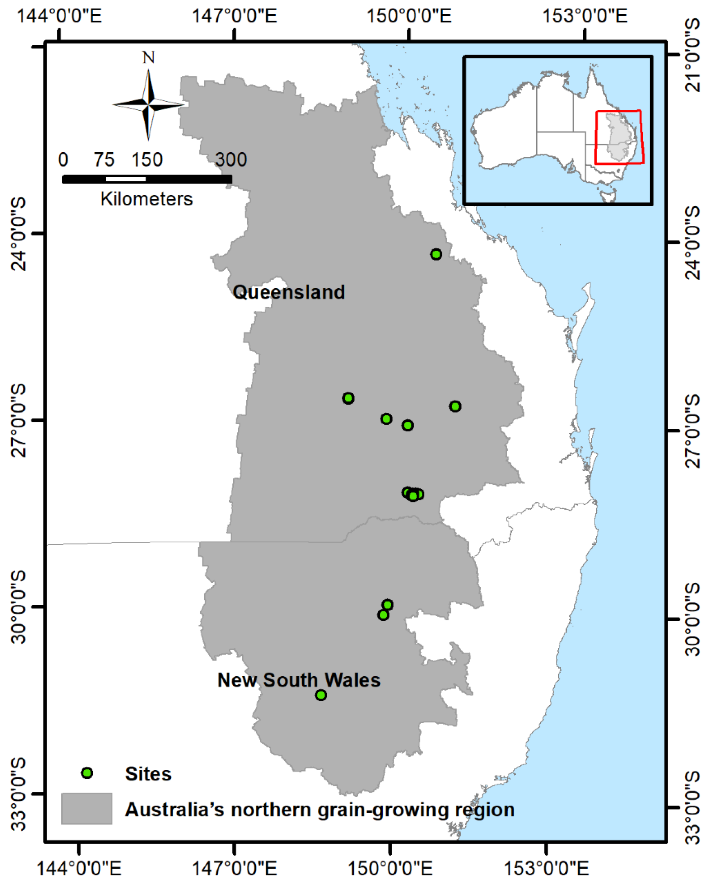
2.1. Study Area

The study area is in Australia’s northern grain-growing region (as defined by the Grains Research and Development Corporation of Australia, GRDC), encompassing Queensland and New South Wales (Figure 1). This work focuses on the winter wheat crop, commonly planted from April to July and harvested from September into December.

2.2. Datasets and Pre-Processing

2.2.1. Crop Yield Monitored Data

This study used 48 wheat yield maps collected from 23 fields between 2001 to 2016. The original yield monitor data were cleaned and block kriged to 30-m grids in previous work [12]. A subset of those data used, as some of them were excluded because (i) there appeared to be differential within-field management (since our ultimate interest with undertaking the current study is the within-field variation of soil constraints, which would be confounded by the presence of within-field variation in management); or (ii) there was a substantial portion of missing values. This pre-processing resulted in the 48 yield maps summarised in Table 1.

2.2.2. Satellite Data

The imagery used in this work are from Landsat-5 Thematic Mapper (TM), Landsat-7 Enhanced Thematic Mapper Plus (ETM+), and Landsat-8 Operational Land Imager (OLI) were collected between 2001 to 2016. Standardised surface reflectance was derived according to [23], and cloud and cloud-shadow were masked from images using the Fmask algorithm [24]. The data all sit on grids with 30-m spacings, and here the data from six bands of each satellite were used, representing the blue, green, red, near-infrared, and two shortwave infrared portions of the electromagnetic spectrum. Only images with at least 75% coverage of each yield map’s pixels were included; images with cloud coverage of more than 25% of a yield map were excluded. Incomplete images occurred because of either (i) partial cloud coverage or (ii) the ‘SLC (Scan Line Corrector)-off’ issue with Landsat-7. Where images were incomplete but had ≥75% coverage, gaps were filled by regression kriging as follows. First, the image (from the same season as the incomplete image) with the highest correlation with the incomplete image was selected as the covariate (provided it covered the missing pixels). Next, a linear model was fitted to predict the missing pixels before the residuals from this linear model were kriged and added to the linear function to give the fill values.

2.2.3. Selection of Vegetation Indices

Eight vegetation indices were tested for studying within-field yield variation. A study by [7] classified the indices into two groups, including indices that provide a representation of canopy structure (VISTR) and indices that are good for describing crop photosynthetic activities (VICHL). The indices are shown in Table 2.
The VISTR indices, NDVI, EVI, EVI2, RVI, VARIgreen, and DVI, represent the canopy structure and are positively correlated with leaf area index (LAI) and biomass. They are formulated based on the captured light within the visible and near-infrared wavelengths, primarily through positive relationships with vegetation reflective bands, such as NIR and green reflectance, and negative relationships with vegetation absorption bands, such as red and blue reflectance. Based on a literature review, the chosen indices have shown good yield prediction in previous crop analyses. The NDVI is a benchmark because it is the most widely used and known index for vegetation fluctuations. The EVI and EVI2 indices were considered because they are sensitive to very dense biomass, able to reduce the disturbance effect from the canopy background and the atmosphere, reduce aerosol perturbation of leaf chlorophyll, and are less prone to saturation [25]. The RVI is a good predictor of leaf water content and is sensitive to green vegetation, so it is well-correlated with the LAI and leaf biomass [26]. The VARIgreen index is less sensitive to atmospheric effects, is suitable for wheat classification, and has an excellent correlation with biomass variation over the entire wheat growing period, so it will not saturate at high leaf biomass [27,28]. Finally, DVI is sensitive to soil background change [29]. The VICHL indices, CVI and, GCVI, indicate nitrogen supply and are a good predictor for crop yield [7]. They are formulated mostly based on two vegetation reflective bands, the NIR, and green bands, which are primarily reflected by healthy vegetation. Both CVI and GCVI have a high correlation with crop chlorophyll content [30]. On the other hand, GCVI is not saturated at high leaf biomass and has a good relationship with the LAI of cereal crops.

2.2.4. Imagery Selection

This work examined the performance of vegetation indices at different stages, where remotely-sensed imagery would have the most potential to hold information indicative of final crop yields. The duration of these stages was fixed at 25 days to allow data capture from up to three separate Landsat images (potentially data for the same field every 8 days, when two of the Landsat satellites are operational). Each interval was defined relative to each vegetation index’s peak values in a time series of field medians; broadly speaking, these peaks correspond to the greatest biomass period. Therefore, the stages were defined as pre-peak, peak, and post-peak stages. For instance, the peak NDVI stage was defined as the 25-day period centred on the date of the peak field-median NDVI; the pre-peak and post-peak NDVI periods were defined as the preceding and following 25-day periods, respectively. Note that the data representing any stage could be a composite of up to three images from the 25-day period.

2.2.5. Set of Covariates

We created models (see Section 2.3 for modelling details) based on various combinations of vegetation indices and stages. We started with a single index from a single-stage and compared different ways of using information from multiple indices or multiple stages. The combinations investigated in this analysis were:
  • A single index, one stage (e.g., NDVI—peak stage);
  • Two indices from different VI groups (see Table 2), both from the same stage (e.g., a combination of NDVI and CVI in peak stage);
  • A single index, all stages (e.g., NDVI from the pre-peak, peak, and post-peak stages);
  • Combinations selected via a stepwise analysis, see Section 2.3.2, allowing any combinations of vegetation index and stage or raw Landsat bands and stage.

2.3. Statistical Methods for Developing and Assesing the Yield Index

2.3.1. The Linear Mixed-Effect Model

The linear model provides a simple general form for relationships between covariates and yield. Typically, this linear model’s residuals (the data minus the linear function’s predicted values) are assumed to be independent. However, in the context of the yield maps used as training data in this work, this assumption is not appropriate since the errors at locations within any particular yield map will be more closely related than the errors from locations in distinct yield maps. The linear-mixed model framework [31] is designed to represent such data; here, the linear function is referred to as the fixed effects, while the residuals, assumed to be normally distributed with some correlation structure, are referred to as the random-effects. Covariate combinations and yield monitored data were paired at each pixel location. A random-effects component (random intercept and slopes) was included for each specific yield map. Models were fitted using the lme4 [32] package for R 4.0.2 [33].

2.3.2. Stepwise Analysis

As noted previously, in addition to manually selected covariates, a stepwise analysis was applied to select combinations of up to six covariates to predict yield. This work used a well-known model-selection criterion, namely the Akaike Information Criterion (AIC) [34], to determine the covariate to be added to the linear-mixed model at each step of the algorithm. This resulted in six models (from the six steps) of increasing complexity. The lower the AIC, the better the fitted model. However, model assessment via cross-validation (see Section 2.3.3) was still applied to each of the six models to provide a better indication of predictive performance.

2.3.3. Cross-Validation

Predictions from the linear-mixed model approach were assessed using a form of cross-validation; this was done for all sets of manually selected covariates (see Section 2.2.5) and for the sets of covariates from each step of the stepwise analysis (Section 2.3.2). Since this work’s main aim was to investigate approaches to predict and map within-field yield variation based on remote-sensing data, a leave-one-yield-map-out cross-validation [8,12] method was adopted (which this work refers to from here on as simply cross-validation). In this approach, each of the 48 yield maps, in turn, was withheld from the training dataset and a linear-mixed model fitted based on the remaining training data. The concordance correlation coefficient [35] was used to assess the relationship between observed and predicted values of the withheld data. The CCC can range from −1 to 1, where the closer the value to 1, the closer the agreement between observed and predicted values, and values close to 0 indicate a lack of association between observed and predicted values. The CCC was first calculated based on the agreement between observed and predicted yields, CCCY. Since a primary objective in this work was to determine how well the predictions represent the spatial patterns of within-field variation of yield, the CCC was also calculated based on the agreement between ranked predictions and ranked withheld data (i.e., the n withheld data, representing all the pixels within any given yield map, were ranked from 1 to n, as were the predictions of these data), referred to here as CCCRank. The CCCRank measures the agreement between pixel rankings based on observed and predicted yields, and as such provides a way to assess how well the high predicted yields corresponded with high actual yields, and the low predicted yields corresponded with low actual yields; in this work, it is this measure that this work focus on most. Each of these measures was calculated for each withheld yield map in turn, and the spread of the 48 CCC values was summarised.
In addition to assessing predictions for any given year, an approach to investigate predictions of longer-term average yields was also applied. Our dataset included 15 fields with more than one year of yield data (Table 1). For a given field with yield maps from T years, a total of P pixels were identified that were present in all T yield maps. The withheld data and predictions for this field were labelled as y p t and y ^ p t (for p in 1 , , P and t in 1 , , T ), respectively. Then the predictions (for each of the P pixels) of the T-year average yield were calculated as the average of y ^ p t over the T years, and compared with the average of y p t over the T years (again using CCCRank). For simplicity, this validation measure was applied only in the final comparison of the validation study.

3. Results

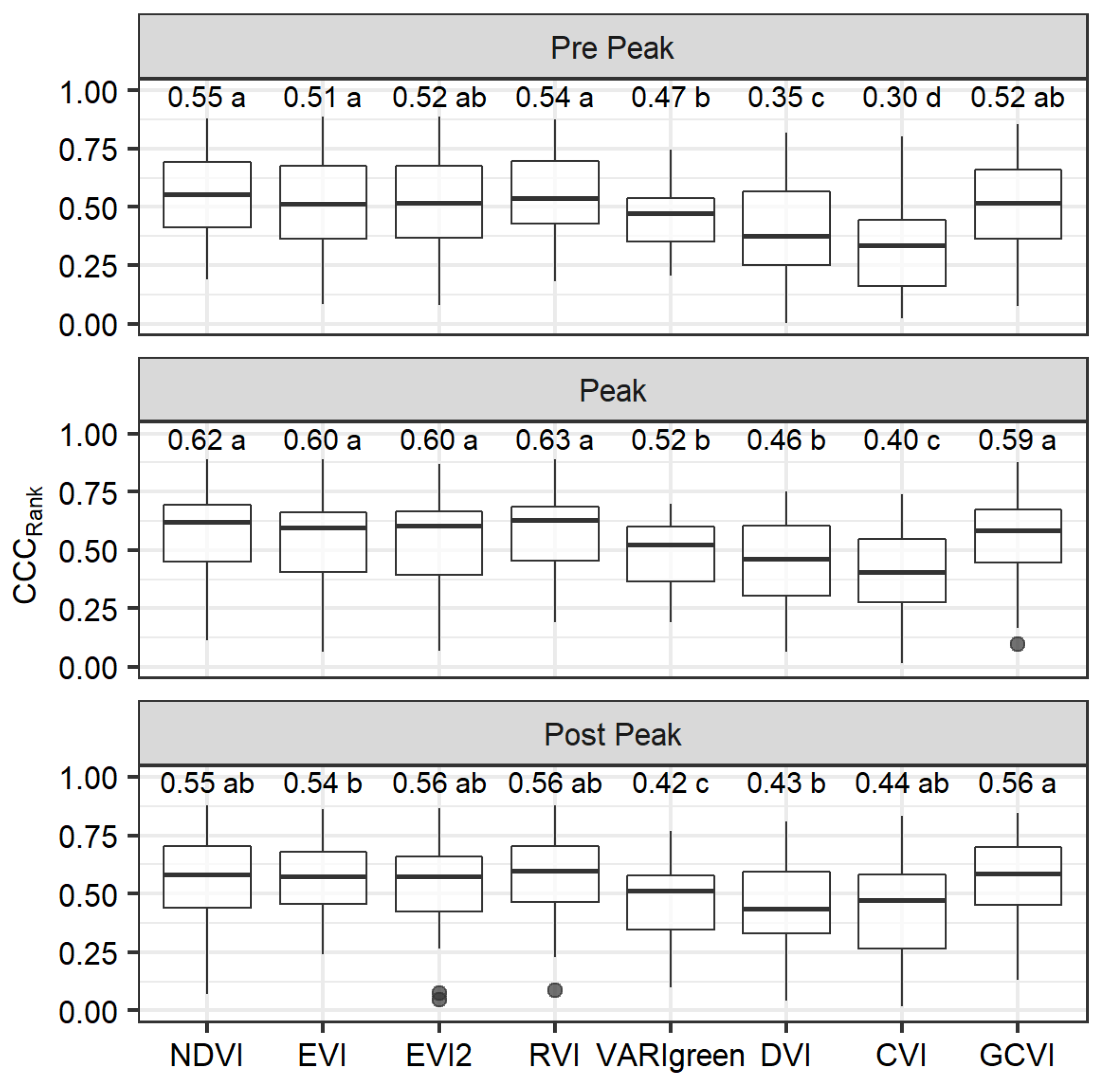
3.1. Single-Index Models

This work applied cross-validation for models based on a single vegetation index in each stage (pre-peak, peak, and post-peak). In most cases, using vegetation index data from the peak stage gave the highest median CCCRank (Figure 2). From the peak stage, NDVI, EVI, EVI2, RVI (all from the VISTR group of indices), and GCVI (from the VICHL group) gave the highest median CCCRank values (0.59–0.63), all giving reasonably similar results. Table 3a shows another performance metric (CCCY) for the models with the five largest CCCRank values. The values of the median CCCY were all less than 0.2, indicating that predictions of actual yield were not very reliable.

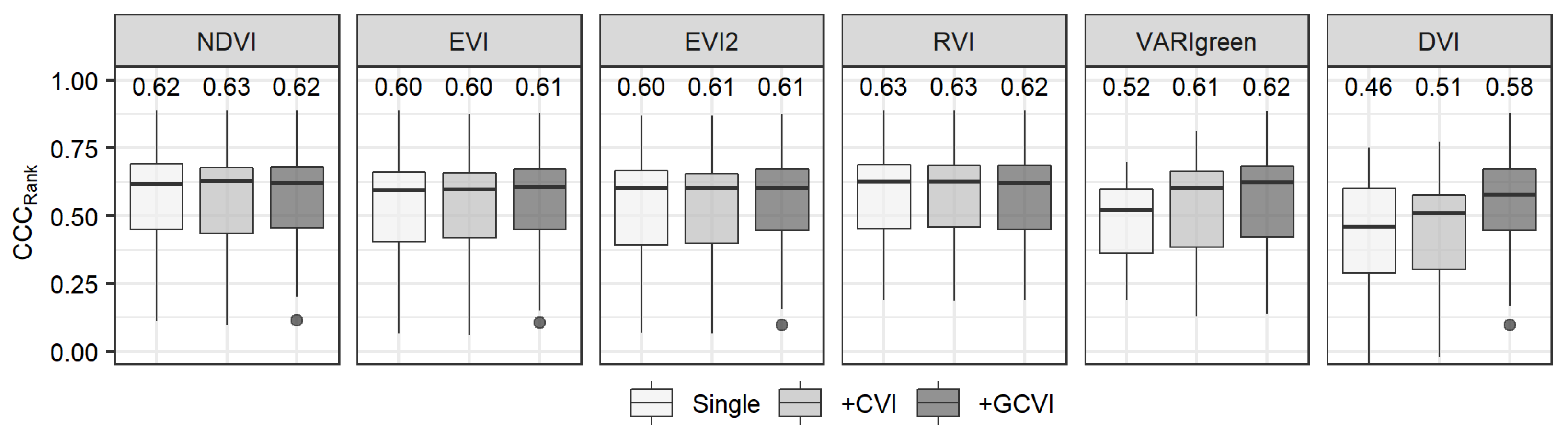
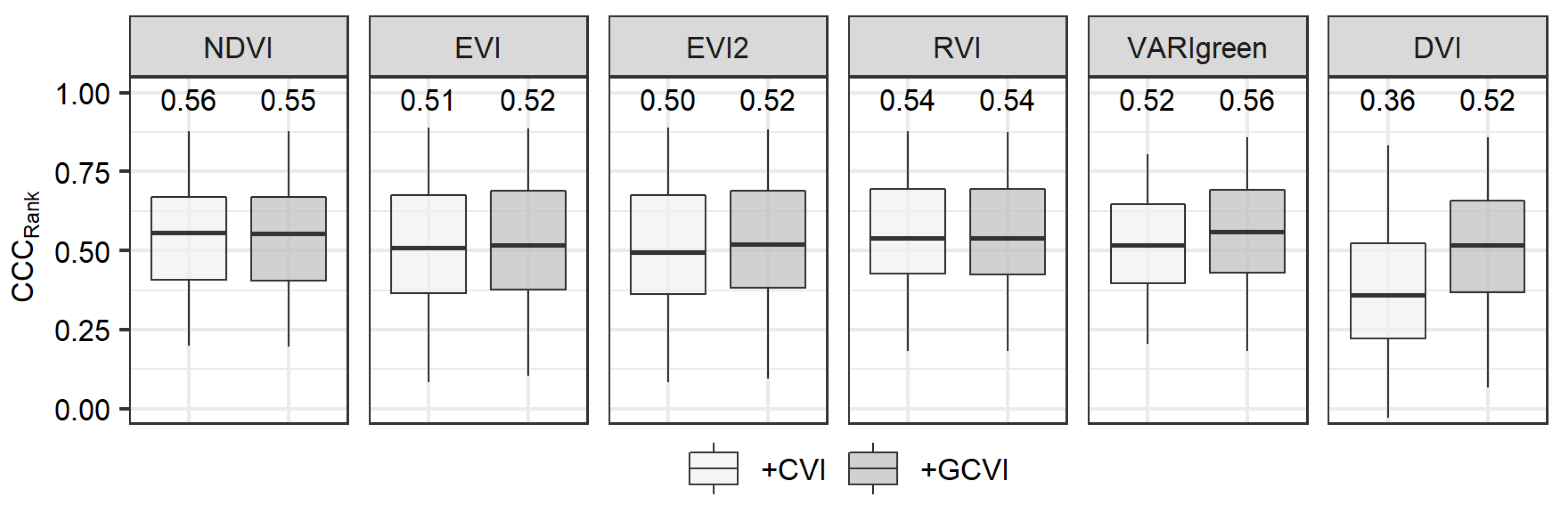
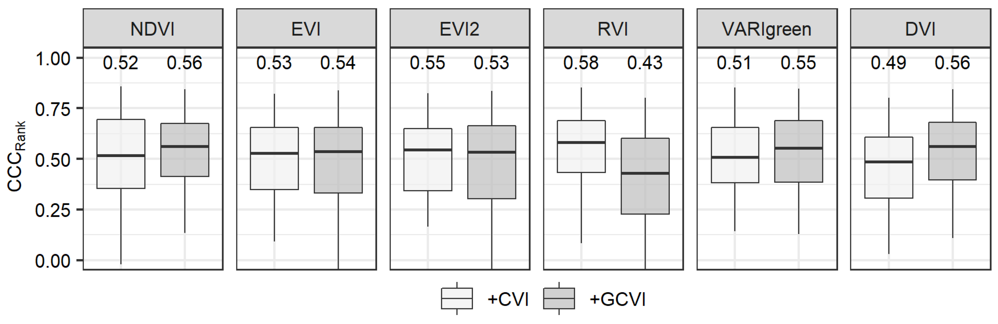
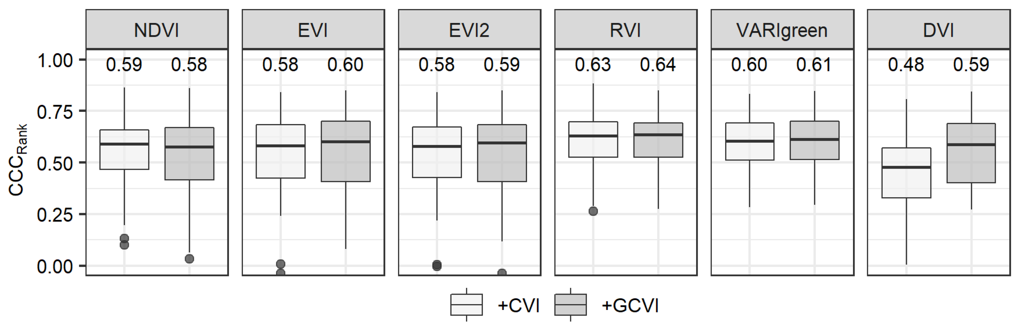
3.2. Multi-Index Models

Multi-index models were assessed for combinations of indices from the two vegetation index groups; six VISTR and two VICHL indices (Figure 3; see Appendix A and Appendix B for the full results). Similarly, to the single-index analysis, all VISTR-VICHL combinations showed the best performance in the peak stage. In this stage, there were generally only small differences between models based on the different indices. Furthermore, the results did not show any notable improvements over those based on a single vegetation index, with the best median CCCRank value being 0.63. This was also the case in terms of CCCY (Table 3b), which showed similar ranges of values to those from the single-index analysis.

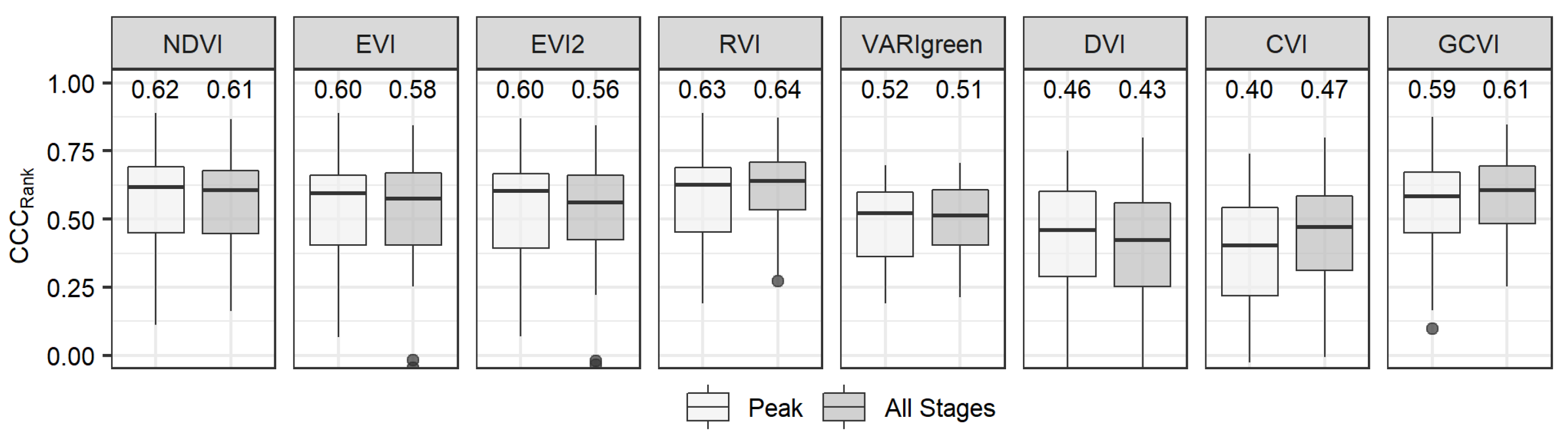
3.3. Multi-Stages Model

In the multi-stage analysis, this work used data from a single vegetation index from all three stages (pre-peak, peak, and post-peak) in the same model. Similarly, in the single-stage analysis, the multi-stage analysis also showed only relatively small differences in CCCRank between indices (Figure 4; see Appendix C for full results). Most of the indices showed a slightly better agreement in the peak stage alone, rather than in the multi-stage analysis (NDVI, EVI, EVI2, VARIgreen, and DVI). This was also the case in terms of actual yield predictions (assessed by the median CCCY; Table 3c).

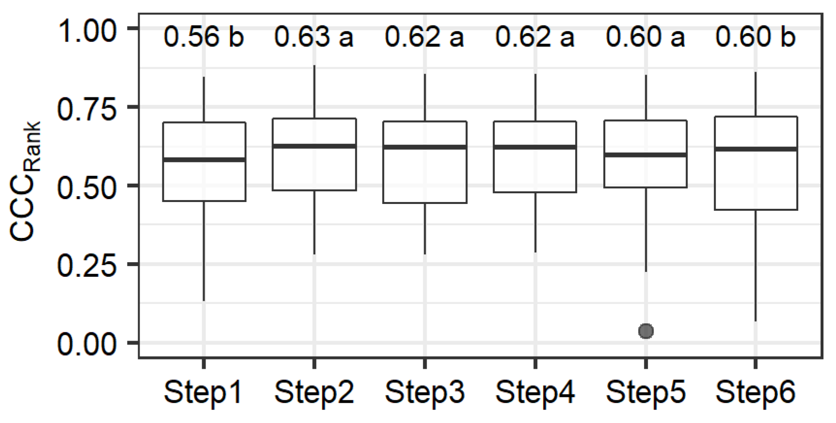
3.4. Stepwise Analysis

Aside from the analyses that used manually selected covariates (a single-index, multiple indices, and multiple stages), this work also applied a stepwise method to select models with up to six covariates. The covariates involved were selected based on the lowest AIC among all the models and subsequently assessed using cross-validation. The first covariate selected was GCVI from the post-peak stage (Table 4), which gave a median CCCRank of 0.56 (Table 3d and Figure 5). The variables selected in the second and third steps were from the pre-peak and peak stages, which improved the median CCCRank value to over 0.6. At the fifth and sixth steps, data from the SWIR1 band were selected, first from the post-peak stage, and next from the peak stage. Cross-validation results from the models selected in steps two, three, four, and five were not significantly different (Figure 5). Based on the cross-validation results, the model from step two, which involved the combination of GCVI post-peak and EVI pre-peak, gave the largest median CCCRank (0.63). This was still no better than the best model from the single-stage analysis (RVI Peak), indicating no better representation of the spatial pattern of yield. In terms of actual yield predictions, results did improve slightly but the best median CCCY values were only around 0.2 (Table 3d). Results showed the best models when considering both metrics were those from Steps 2–4 of the stepwise algorithm, which showed CCC values close or similar to those of the best model in terms of CCCRank (RVI Peak, GCVI post-peak, and EVI pre-peak) and in terms of CCCY (NDVI peak).

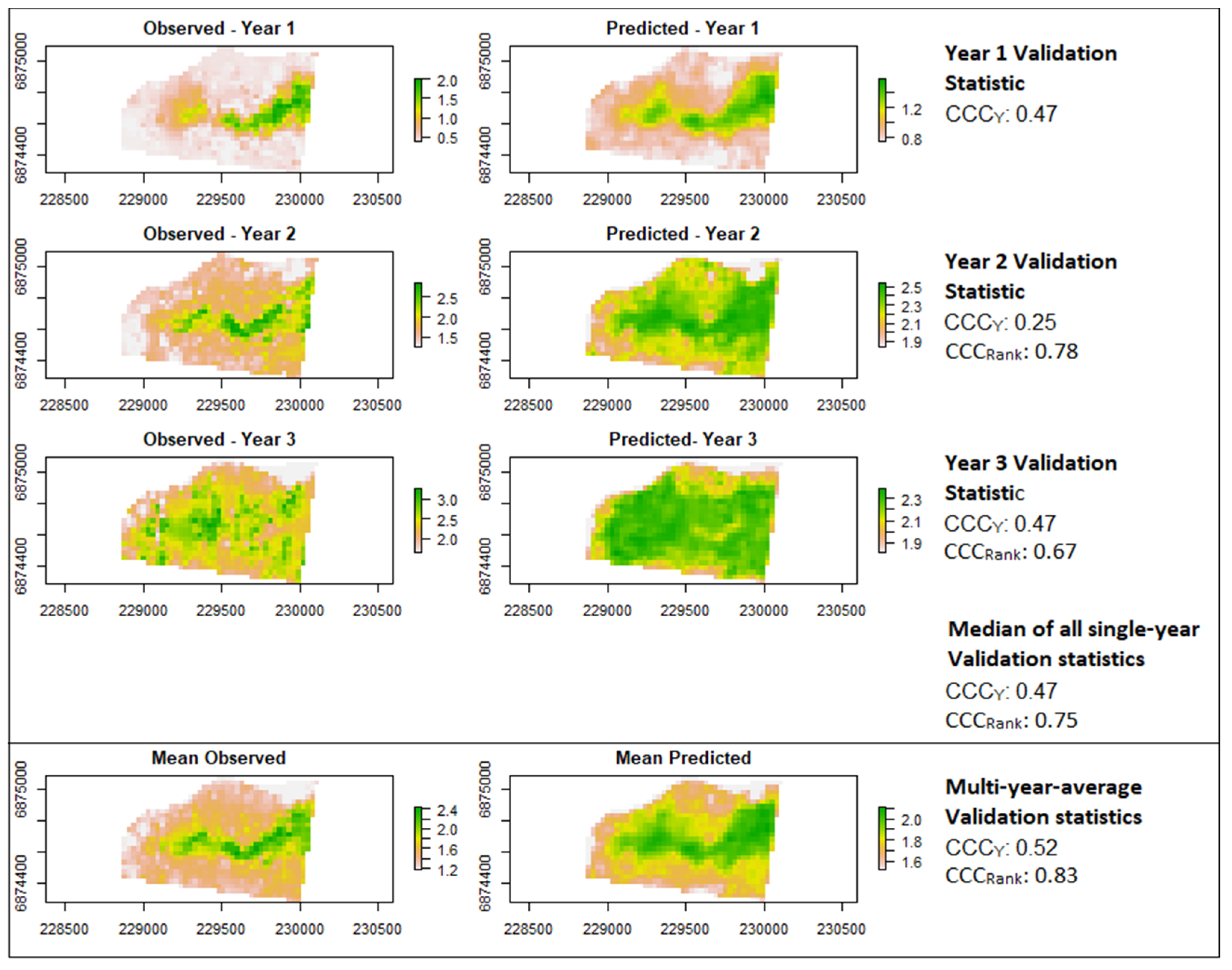
3.5. Comparing Multi-Year Average Prediction and Single Year Prediction

A performance measure was calculated for fields with more than one year of yield data. For this analysis, this work focused on just the model of NDVI peak because it was considered as a well-known vegetation index and had quite a high median CCCRank compared to other models. As shown in the three years of data, similar spatial patterns of yield were observed (and predicted) for all three years. In this field, there were 825 pixels in all three years, and only these common pixels are analysed here and shown in Figure 6.
The validation statistics for a single year showed large differences in CCCY and CCCRank between years. The CCCY values for the first and the third year were 0.47, while the second year was 0.25, giving a median CCCY value of 0.47 over the three years. The CCCRank values showed smaller differences between years, with the highest CCCRank value occurring for the second-year data (0.78), then followed by the first and third-year results (0.75 and 0.67), giving a median CCCRank value of 0.75 over the three years.
These median values (0.47 for CCCY and 0.75 for CCCRank) indicate how well yields for individual years were predicted in this field. An indication of how well longer-term average yields were predicted is provided by directly comparing the three-year-average maps (those on the final row of Figure 6); the CCCY and CCCRank for the three-year-average maps were 0.52 and 0.83, respectively.
Results in Figure 6 illustrate the process of multi-year validation for one field; Table 5 summarises the results from similar analyses of all 15 fields where multi-year data were available. The table shows that all the final mean and median CCC values for both metrics were larger in the multi-year analysis than in the single-year analysis. In particular, the CCCRank from the multi-year analysis was on average 0.12higher than that from the single-year analysis (p < 0.05, from a paired t-test). Moreover, over the 15 fields analysed for Table 5, the CCCRank for individual fields ranged from 0.11 (Field 3, Year 2008) to 0.89 (Field 9, Year 2002), whereas the multi-year CCCRank values ranged from 0.42 for Field 3 to 0.86 for Field 13. Thus, the multi-year results suggest that using multi-year predictions reduces the risk of very poor predictions.

4. Discussion

4.1. Selection of Vegetation Indices and Stages for Simple Yield-Prediction Models

Several of the vegetation indices tested performed similarly in terms of the median CCCRank. Figure 2 depicts this similarity for the best five CCCRank within all stages (NDVI, EVI, EVI2, RVI, and GCVI). All five indices ranged from 0.51–0.55 during the pre-peak stage, 0.59–0.63 during the peak stage, and 0.54 to 0.56 during the post-peak stage. These top five models came from both groups of indices, where NDVI, EVI, EVI2, and RVI are categorised as canopy structural-related indices (VISTR), and GCVI is a chlorophyll-related index (VICHL). Thus, this study did not find any evidence to suggest that there is an advantage to using a canopy structural-related index (VISTR) over a chlorophyll-related index (VICHL) or vice versa. A previous study from [7] also reported similar findings, where the VISTR and VICHL gave a similar performance for predicting actual wheat yields.
Two possible ways of incorporating extra information (compared with a single-index, single-stage model) were investigated: using data from two different vegetation indices (one canopy structural-related index and one chlorophyll-related index, both from the same stage; multi-index models) and using data from all stages (for the same vegetation index; multi-stage models). Neither of these approaches resulted in large improvements in predictions (a best value of CCCRank of 0.63 from the multi-index models and of 0.64 for the multi-stage models) compared with the single-index single-stage models. A similar result was also reported by [7], who also found only a small increase in predictive power when assessing a combination of structural and chlorophyll-related indices [7] assumed that this similarity occurred because structural and chlorophyll-related indices respond to different aspects of the crop (morphological and physiological). In our study, one possible reason for the lack of improvement might be the overlap in information (correlation) between the vegetation index data from the same index (different stages) or from the same stage (different indices). However, results from a stepwise analysis—where data from different vegetation indices, different stages, and the raw Landsat bands could be added to the model—also gave a best value of the median CCCRank of 0.63. In this case, the information added to the model at each step would not be so correlated with information already in the model. Therefore, results here (based on this dataset of yield monitor data and the pool of simple linear models of vegetation indices tested) suggest linear functions of a single vegetation index (any of NDVI, EVI, EVI2, RVI, and GCVI) from around the time of its season peak would give reasonably accurate representations of the spatial patterns of within-field yield variation (a median CCCRank of around 0.6).

4.2. Another Metric Assesing Properties of Yield Predictions

In terms of actual yield predictions, the best value of the median CCCY was only 0.2. The validation statistics in terms of this metric were smaller than for yield rankings because it is more challenging to predict actual yields and their within-field variation (based on just remote-sensing data) than to predict the within-field yield rankings. One possible reason for the very modest results in terms of CCCY (in comparison with other studies, e.g., [7]) is the cross-validation approach used. This form of cross-validation would provide a sterner and more relevant prediction test than internal metrics (e.g., R2) or cross-validation with random splitting. Other studies also recommended the use of this cross-validation strategy since it provides a realistic and accurate prediction [3,4]. In any case, the results indicated that the predictions of actual yield for any single year, based on the models involved in this work, should be used cautiously.

4.3. Stepwise Results Revealed Some Simple Models

Initially, this work hypothesised that the best single-covariate model would be one consisting of a vegetation index coming from the peak stage. In terms of the median CCCRank from cross-validation (Figure 2), our results backed up this hypothesis. However, the first variable to be added in the stepwise analysis was GCVI from the post-peak stage, which gave the smallest AIC of all the single-covariate models. Although selected based on the AIC, this model did not perform so well in terms of the median CCCRank from cross-validation; this highlights the importance of validation methods and metrics tailored to assess the properties that are considered most important for a particular application, which in this case was defined as an assessment of spatial patterns of within-field yield variation.
There were two interesting observations that can be made from this stepwise analysis: (i) the first three covariates to be added were all different vegetation indices from different stages and (ii) the peak stage information was not included until step three. The first three indices were GCVI post-peak, EVI pre-peak, and EVI2 peak. A possible reason is that there might be overlapping information in different vegetation indices from the same stage or in the same vegetation index from different stages. Therefore, the most useful models include different indices and different stages. Furthermore, in steps 5 and 6, data from a raw band (SWIR1) were added to the model. The selection of SWIR1 was possibly because, in the previous steps, all the vegetation indices added to the model were formulated from the visible and NIR bands. Therefore, the SWIR1 band might provide additional information, such as moisture information [36], that was not included in the previous steps.
In terms of CCCRank, there was no notable improvement from the stepwise models (Table 3d) compared with the single-index models (Table 3a). However, in terms of CCCY, the cross-validation results suggested that the models from steps 2–4 gave the best all-around performance. The CCCY values were around 0.2, which were slightly higher than other model performances. Therefore, if one is willing to use a model of more than a single index, then one of these models might be preferable.

4.4. Multi-Year Analyses and Implications

There are many possible reasons for poor prediction performance. Notably, for a particular year, there could be issues with the yield monitor data or with the failure of the remote-sensing data to capture the information most relevant to yield variation (because of the timing of imagery or an index that is not sensitive within a particular field and date). These issues can lead to predictions that show a good correlation with the data for a particular year, but a poor correlation for the same field in other years. Therefore, in this work, a long-term-average analysis was also applied for some fields that presented more than one year of yield data (fields with two or three years in our dataset). The multi-year yield analysis (applied with the NDVI peak single-covariate model) showed that the mean and median of both metrics were better for the multi-year than for the single-year results. These results suggested that a single year’s validation might provide a conservative assessment of long-term-average yield prediction performance. In terms of the mean over all the multi-year fields, the improvement from the multi-year results was 0.05 for CCCY and 0.12 for CCCRank.
Based on these multi-year improvements, it might be reasonable to expect predictions of averages over more years, such as five or ten years (our dataset had fields with at most three years of data), to give larger improvements. Besides, the results also give confidence that predictions from remote-sensing vegetation indices over multiple years are a valuable tool for precision agriculture to reveal consistent spatial patterns in yield. Previous studies [2,37] have used consistent yield patterns to target soil sampling to identify the reason behind the low yielding areas; given that persistently low yield can indicate the presence of a soil constraint. Therefore, the methodology identified from this work could be used to develop tools to provide growers with important information about the potential presence and location of soil constraints on a paddock scale. In further work, the current analysis will be built on by using predictions based on models in this paper together with data on other factors that potentially drive the spatial variation on crop yield (e.g., topography, climate, soil).

5. Conclusions

This work concluded that there were only marginal differences in the performance of the different vegetation indices tested. The well-known indices, such as NDVI, RVI, EVI, and EVI2, mostly showed good predictions of the spatial pattern of yield, but only modest performance in terms of predictions of actual yield (when assessed via within-field metrics with leave-one-yield-map-out cross-validation). In terms of vegetation index group, indices from both the structural-related group (VISTR) and the chlorophyll-related group (VICHL) gave a similar performance in the single-index, single-stage analysis. In terms of stages, data from the peak stage gave the best performance, and combining data from the same vegetation index but from multiple stages did not improve predictions. Results from a stepwise analysis revealed some simple combinations of different vegetation indices from different stages could have better predictions in terms of actual yield predictions but did not improve over the single-index models in terms of yield ranking predictions alone. Moreover, the results showed that longer-term average yield predictions were generally more accurate than those of yield for single years, and also reduced the risk of having predictions with poor performance.

Author Contributions

Conceptualization: F.U., T.G.O., Y.P.D. and N.W.M.; methodology: F.U. and T.G.O.; analysis and result interpretation: F.U. and T.G.O.; writing—original draft preparation: F.U.; writing—review and editing: T.G.O., Y.P.D. and N.W.M. All authors have read and agreed to the published version of the manuscript.

Funding

This work was funded by the Grains Research and Development Corporation (GRDC) of Australia under project number UOQ1803-003RTX.

Data Availability Statement

The datasets generated during and/or analysed during the current study are available from the corresponding author on reasonable request.

Acknowledgments

This research was supported and funded by the Grains Research and Development Corporation (GRDC) of Australia under project number UOQ1803-003RTX. The authors also thank for helpful discussions from Scott Chapman and Yunru Lai.

Conflicts of Interest

The authors declare that they have no conflict of interest.

Appendix A

Figure A1. The concordance correlation coefficients of ranks for models with two vegetation indices in the pre-peak stage. Values show the median CCCRank. For better visualisation, the figure excludes negative CCCRank.
Agronomy 12 00384 g0a1

Appendix B

Figure A2. The concordance correlation coefficients of ranks for models with two vegetation indices in the post-peak stage. Values show the median CCCRank. For better visualisation, the figure excludes negative CCCRank.
Agronomy 12 00384 g0a2

Appendix C

Figure A3. The concordance correlation coefficients of ranks for multi-stages and multi-index analysis. Values show the median CCCRank for each treatment. For better visualisation, the figure excluded negative CCCRank.
Agronomy 12 00384 g0a3

References

  1. Cai, Y.; Guan, K.; Lobell, D.; Potgieter, A.B.; Wang, S.; Peng, J.; Xu, T.; Asseng, S.; Zhang, Y.; You, L.; et al. Integrating satellite and climate data to predict wheat yield in Australia using machine learning approaches. Agric. For. Meteorol. 2019, 274, 144–459. [Google Scholar] [CrossRef]
  2. Dang, Y.P.; Pringle, M.J.; Schmidt, M.; Dalal, R.C.; Apan, A. Identifying the spatial variability of soil constraints using multi-year remote sensing. Field Crop. Res. 2011, 123, 248–258. [Google Scholar] [CrossRef]
  3. Dang, Y.P.; Dalal, R.C.; Christopher, J.; Apan, A.A.; Pringle, M.J.; Bailey, K.; Biggs, A.J.W. Managing Subsoil Constraints Advanced Techniques for Managing Subsoil Constraints Project Results Book; Grains Research & Development Corporation: Canberra, ACT, Australia, 2010. [Google Scholar]
  4. Wulder, M.A.; Masek, J.G.; Cohen, W.B.; Loveland, T.R.; Woodcock, C.E. Opening the archive: How free data has enabled the science and monitoring promise of Landsat. Remote Sens. Environ. 2012, 122, 2–10. [Google Scholar] [CrossRef]
  5. Tucker, C.J. Red and photographic infrared linear combinations for monitoring vegetation. Remote Sens. Environ. 1979, 8, 127–150. [Google Scholar] [CrossRef] [Green Version]
  6. Huete, A.; Didan, K.; Miura, T.; Rodriguez, E.; Gao, X.; Ferreira, L. Overview of the radiometric and biophysical performance of the MODIS vegetation indices. Remote Sens. Environ. 2002, 83, 195–213. [Google Scholar] [CrossRef]
  7. Zhao, Y.; Potgieter, A.B.; Zhang, M.; Wu, B.; Hammer, G.L. Predicting wheat yield at the field scale by combining high-resolution Sentinel-2 satellite imagery and crop modelling. Remote Sens. 2020, 12, 1024. [Google Scholar] [CrossRef] [Green Version]
  8. Filippi, P.; Jones, E.J.; Wimalathunge, N.S.; Somarathna, P.D.S.N.; Pozza, L.E.; Ugbaje, S.U.; Jephcott, T.G.; Paterson, S.E.; Whelan, B.M.; Bishop, T.F.A. An approach to forecast grain crop yield using multi-layered, multi-farm data sets and machine learning. Precis. Agric. 2019, 20, 1015–1029. [Google Scholar] [CrossRef]
  9. Basso, B.; Ritchie, J.T.; Pierce, F.J.; Braga, R.P.; Jones, J.W. Spatial validation of crop models for precision agriculture. Agric. Syst. 2001, 68, 97–112. [Google Scholar] [CrossRef]
  10. Colwell, J.E.; Rice, D.P.; Nalepka, R.F. Wheat yield forecasts using Landsat data. In Proceedings of the Eleventh International Symposium on Remote Sensing of Environment, Ann Arbor, MI, USA, 25–29 April 1977; pp. 1245–1254. [Google Scholar]
  11. Kastens, J.H.; Kastens, T.L.; Kastens, D.L.A.; Price, K.P.; Martinko, E.A.; Lee, R.Y. Image masking for crop yield forecasting using AVHRR NDVI time series imagery. Remote Sens. Environ. 2005, 99, 341–356. [Google Scholar] [CrossRef]
  12. Lai, Y.R.; Pringle, M.J.; Kopittke, P.M.; Menzies, N.W.; Orton, T.G.; Dang, Y.P. An empirical model for prediction of wheat yield, using time-integrated Landsat NDVI. Int. J. Appl. Earth Obs. Geoinf. 2018, 72, 99–108. [Google Scholar] [CrossRef]
  13. Yang, C.; Everitt, J.H.; Bradford, J.M. Airborne hyperspectral imagery and linear spectral unmixing for mapping variation in crop yield. Precis. Agric. 2007, 8, 279–296. [Google Scholar] [CrossRef]
  14. Al-Gaadi, K.A.; Hassaballa, A.A.; Tola, E.; Kayad, A.G.; Madugundu, R.; Alblewi, B.; Assiri, F. Prediction of potato crop yield using precision agriculture techniques. PLoS ONE 2016, 11, e0162219. [Google Scholar] [CrossRef]
  15. Bai, T.; Zhang, N.; Mercatoris, B.; Chen, Y. Jujube yield prediction method combining Landsat 8 vegetation index and the phenological length. Comput. Electron. Agric. 2019, 162, 1011–1027. [Google Scholar] [CrossRef]
  16. Goodwin, A.W.; Lindsey, L.E.; Harrison, S.K.; Paul, P.A. Estimating wheat yield with normalized difference vegetation index and fractional green canopy cover. Crop. Forage Turfgrass Manag. 2018, 4, 1–6. [Google Scholar] [CrossRef] [Green Version]
  17. Hancock, D.W.; Dougherty, C.T. Relationships between blue-and red-based vegetation indices and leaf area and yield of alfalfa. Crop Sci. 2007, 47, 2547–2556. [Google Scholar] [CrossRef]
  18. Jurečka, F.; Lukas, V.; Hlavinka, P.; Semerádová, D.; Žalud, Z.; Trnka, M. Estimating crop yields at the field level using landsat and modis products. Acta Univ. Agric. Silvic. Mendel. Brun. 2018, 66, 1141–1150. [Google Scholar] [CrossRef] [Green Version]
  19. Liu, L.; Wang, J.; Bao, Y.; Huang, W.; Ma, Z.; Zhao, C. Predicting winter wheat condition, grain yield and protein content using multi-temporal EnviSat-ASAR and Landsat TM satellite images. Int. J. Remote Sens. 2006, 27, 737–753. [Google Scholar] [CrossRef]
  20. Lobell, D.B.; Asner, G.P. Comparison of earth observing-1 ALI and Landsat ETM+ for crop identification and yield prediction in Mexico. IEEE Trans. Geosci. Remote Sens. 2003, 41, 1277–1282. [Google Scholar] [CrossRef]
  21. Mokhtari, A.; Noory, H.; Vazifedoust, M. Improving crop yield estimation by assimilating LAI and inputting satellite-based surface incoming solar radiation into SWAP model. Agric. For. Meteorol. 2018, 250–251, 159–170. [Google Scholar] [CrossRef]
  22. Sulik, J.J.; Long, D.S. Spectral considerations for modeling yield of canola. Remote Sens. Environ. 2016, 184, 161–174. [Google Scholar] [CrossRef] [Green Version]
  23. Flood, N.; Danaher, T.; Gill, T.; Gillingham, S. An operational scheme for deriving standardised surface reflectance from landsat TM/ETM+ and SPOT HRG imagery for eastern Australia. Remote Sens. 2013, 5, 83–109. [Google Scholar] [CrossRef] [Green Version]
  24. Zhu, Z.; Wang, S.; Woodcock, C.E. Improvement and expansion of the Fmask algorithm: Cloud, cloud shadow, and snow detection for Landsats 4–7, 8, and Sentinel 2 images. Remote Sens. Environ. 2015, 159, 269–277. [Google Scholar] [CrossRef]
  25. Liu, J.; Pattey, E.; Jégo, G. Assessment of vegetation indices for regional crop green LAI estimation from Landsat images over multiple growing seasons. Remote Sens. Environ. 2012, 123, 347–358. [Google Scholar] [CrossRef]
  26. Wei, C.; Huang, J.; Wang, X.; Blackburn, G.A.; Zhang, Y.; Wang, S.; Mansaray, L.R. Hyperspectral characterization of freezing injury and its biochemical impacts in oilseed rape leaves. Remote Sens. Environ. 2017, 195, 56–66. [Google Scholar] [CrossRef] [Green Version]
  27. Gitelson, A.A.; Viña, A.; Arkebauer, T.J.; Rundquist, D.C.; Keydan, G.; Leavitt, B. Remote estimation of leaf area index and green leaf biomass in maize canopies. Geophys. Res. Lett. 2003, 30. [Google Scholar] [CrossRef] [Green Version]
  28. Kobayashi, N.; Tani, H.; Wang, X.; Sonobe, R. Crop classification using spectral indices derived from Sentinel-2A imagery. J. Inf. Telecommun. 2020, 4, 67–90. [Google Scholar] [CrossRef]
  29. Richardson, A.J.; Wiegand, C.L. Distinguishing Vegetation from Soil Background Information* A gray mapping technique allows delineation of any Landsat scene into vegetative cover stages, degrees of soil brightness, and water. Photogammetric Eng. Remote Sens. 1977, 43, 1541–1552. [Google Scholar]
  30. Hunt, E.R.; T Daughtry, C.S.; H Eitel, J.U.; Long, D.S. Remote sensing leaf chlorophyll content using a visible band index. Agron. J. 2011, 103, 1090–1099. [Google Scholar] [CrossRef] [Green Version]
  31. Pinheiro, J.; Bates, D. Mixed-Effects Models in S and S-PLUS; Springer: New York, NY, USA, 2006; ISBN 9781441903174. [Google Scholar]
  32. Bates, D.; Maechler, M.; Bolker, B.; Walker, S. Fitting linear mixed-effects models using lme4. J. Stat. Softw. 2015, 67, 1–48. [Google Scholar] [CrossRef]
  33. R Core Team. R: A Language and Environment for Statistical Computing; R Foundation for Statistical Computing: Vienna, Austria, 2020. [Google Scholar]
  34. Akaike, H. Information theory and an extension of the maximum likelihood principle. In Selected Papers of Hirotugu Akaike; Kiado, A., Ed.; Springer: New York, NY, USA, 1998; pp. 199–213. ISBN 9781461272489. [Google Scholar]
  35. Lin, L.I. A Concordance Correlation Coefficient to Evaluate Reproducibility. Biomatrics 1989, 45, 255–268. [Google Scholar] [CrossRef]
  36. Lobell, D.B.; Asner, G.P. Moisture effects on soil reflectance. Soil Sci. Soc. Am. J. 2002, 66, 722–727. [Google Scholar] [CrossRef]
  37. Lobell, D.B.; Ortiz-Monasterio, J.I.; Gurrola, F.C.; Valenzuela, L. Identification of saline soils with multiyear remote sensing of crop yields. Soil Sci. Soc. Am. J. 2007, 71, 777–783. [Google Scholar] [CrossRef] [Green Version]
Figure 1. Study area.
Agronomy 12 00384 g001
Figure 2. The concordance correlation coefficients of ranks for single vegetation indices from a single stage. Values show the median CCCRank for each treatment. For better visualisation, the figure excluded negative CCCRank. Within a stage, vegetation indices with the same letters are not significantly different.
Agronomy 12 00384 g002
Figure 3. The concordance correlation coefficients of ranks for models with two vegetation indices in the peak stage. Values show the median CCCRank. For better visualisation, the figure excludes negative CCCRank.
Agronomy 12 00384 g003
Figure 4. The concordance correlation coefficients of ranks for multi-stages single-index analysis. Values show the median CCCRank for each treatment. For better visualisation, the figure excluded negative CCCRank.
Agronomy 12 00384 g004
Figure 5. The concordance correlation coefficients of ranks for the stepwise analysis. Values show the median CCCRank for each treatment. For better visualisation, the figure excluded negative CCCRank. Steps with the same letters are not significantly different.
Agronomy 12 00384 g005
Figure 6. Single and multi-year yield maps of Field 23. The horizontal and vertical axis of the map are the site coordinates.
Agronomy 12 00384 g006
Table 1. Yield maps involved in the study.
FieldsYearFieldsYear
Field 12007, 2008Field 132002, 2005, 2009
Field 22003, 2008Field 142002, 2005, 2009
Field 32006, 2008Field 152002, 2007, 2009
Field 42015Field 162001
Field 52016Field 172001
Field 62015Field 182001
Field 72009Field 192001, 2005, 2009
Field 82006, 2009Field 202003, 2004
Field 92002, 2005, 2009Field 212002, 2005, 2009
Field 102002, 2005, 2009Field 222001, 2002, 2009
Field 112003Field 232002, 2003, 2007
Field 122003, 2005, 2009
Table 2. Vegetation indices.
IndexEquation
Canopy Structural-Related Indices (VISTR)
Normalised difference vegetation index (NDVI) N I R     R e d N I R   +   R e d
Enhanced Vegetation Index (EVI) 2.5 N I R     R e d N I R   +   6   ×   R e d     7.5   ×   B l u e   +   1
Enhanced Vegetation Index 2 (EVI2) 2.4 N I R     R e d N I R   +   R e d   +   1
Ratio Vegetation Index (RVI) N I R / R e d
Visible Atmospherically Resistant Index Green (VARIgreen) G r e e n     R e d G r e e n   +   R e d     B l u e
Difference Vegetation Index (DVI) 2.4   ×   N I R     R e d
Chlorophyll-related indices (VICHL)
Chlorophyll Vegetation Index (CVI) N I R   ×   R e d G r e e n 2
Green Chlorophyll Vegetation Index (GCVI) ( ( N I R / G r e e n )     1 )
Table 3. Median CCC values from cross-validation based on manually selected covariates and those from the stepwise analysis. Covariates for stepwise models are referred to as S1–S5.
ModelsCCCRankCCCY
(a) 
Single-index analysis
NDVI Peak0.620.19
EVI Peak0.600.13
EVI2 Peak0.600.14
RVI Peak0.630.10
GCVI Peak0.590.11
(b) 
Multi-index analysis
NDVI Peak-CVI Peak0.630.18
RVI Peak-CVI Peak0.630.11
NDVI Peak-GCVI Peak0.620.14
RVI Peak-GCVI Peak0.620.10
VARIgreen Peak-GCVI Peak0.620.13
(c) 
Multi-stage analysis
NDVI All Stages0.610.17
EVI All Stages0.580.13
EVI2 All Stages0.560.13
RVI All Stages0.640.12
GCVI All Stages0.610.16
(d) 
Stepwise Analysis
S1 = GCVI Post Peak 0.560.11
S2 = S1 and EVI Pre Peak0.630.17
S3 = S2 and EVI2 Peak0.620.19
S4 = S3 and VARIgreen Post Peak 0.620.19
S5 = S4 and SWIR1 Post Peak0.600.17
Table 4. AIC summary for models in stepwise analysis. Covariate sets are referred to as S1–S6.
StepsCovariate Added to ModelAIC
1S1 = GCVI Post Peak 3626
2S2 = S1 and EVI Pre Peak−9881
3S3 = S2 and EVI2 Peak−17,753
4S4 = S3 and VARIgreen Post Peak −20,700
5S5 = S4 and SWIR1 Post Peak−22,649
6S6 = S5 and SWIR1 Peak−24,778
Table 5. CCC values from single-year analysis (median of CCC values from individual years) and multi-year results summary.
Single YearLong-Term
FieldsCCCYCCCRankCCCYCCCRank
Field 10.020.640.210.73
Field 20.130.680.120.78
Field 30.020.360.240.42
Field 80.070.630.050.75
Field 90.180.640.250.85
Field 100.170.670.130.67
Field 120.260.570.120.69
Field 130.160.810.210.86
Field 140.130.240.170.47
Field 150.000.240.080.57
Field 190.320.610.310.66
Field 200.270.550.240.62
Field 210.470.740.790.85
Field 220.410.610.480.70
Field 230.470.750.520.83
Median0.170.630.210.70
Mean0.210.580.260.70
Publisher’s Note: MDPI stays neutral with regard to jurisdictional claims in published maps and institutional affiliations.

