
Digital Mapping of Soil Profile Properties for Precision Agriculture in Developing Countries

 ,
, 
Abstract
:1. Introduction
2. Materials and Methods
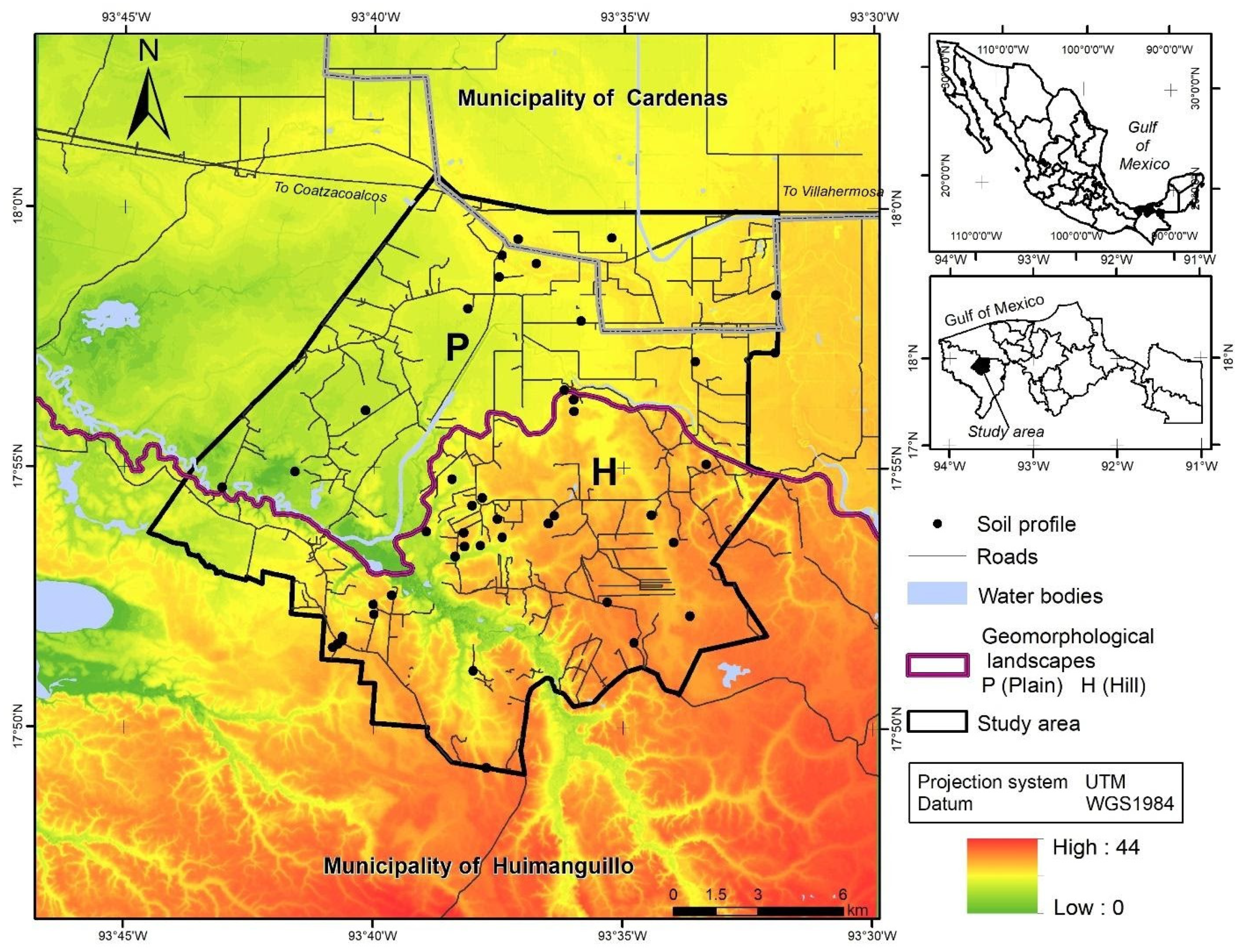
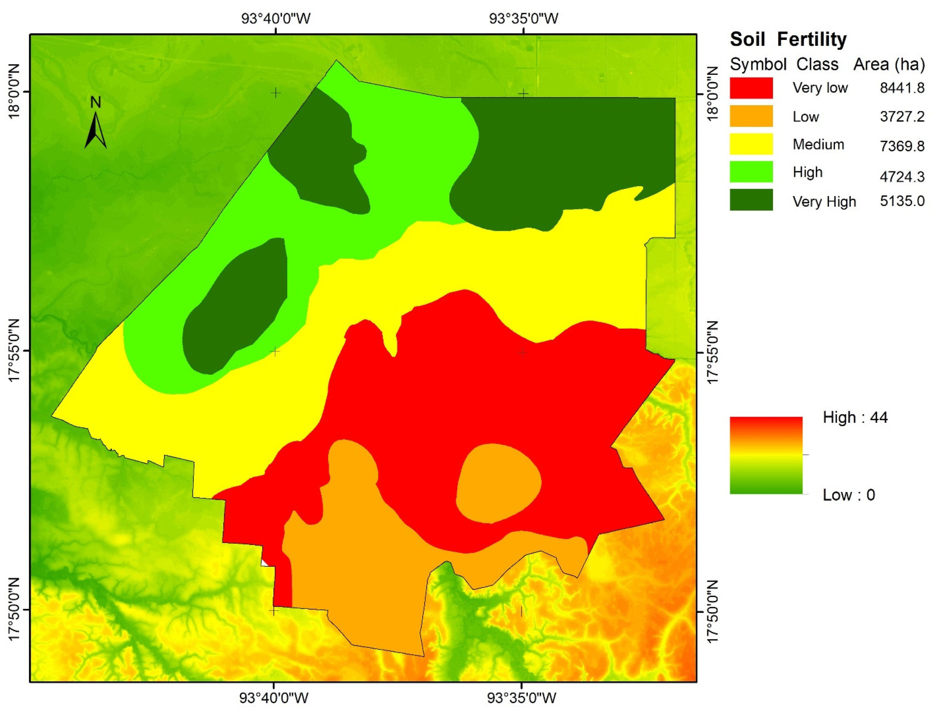
2.1. Study Zone
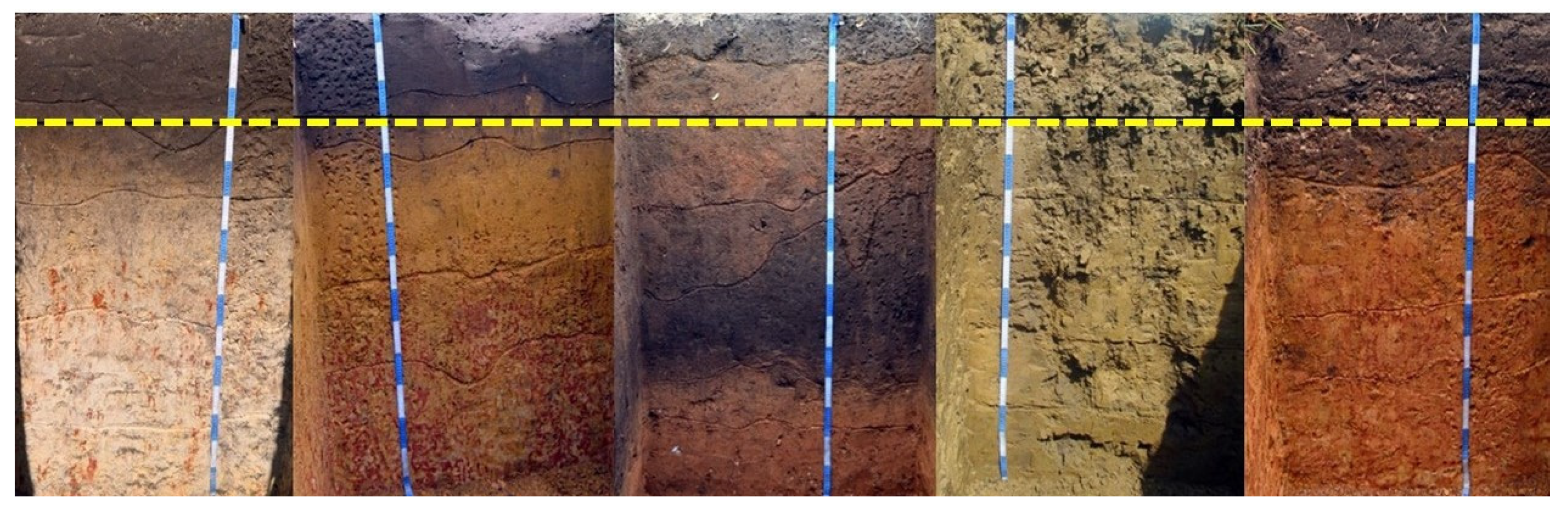
2.2. Soil Sampling and Analysis
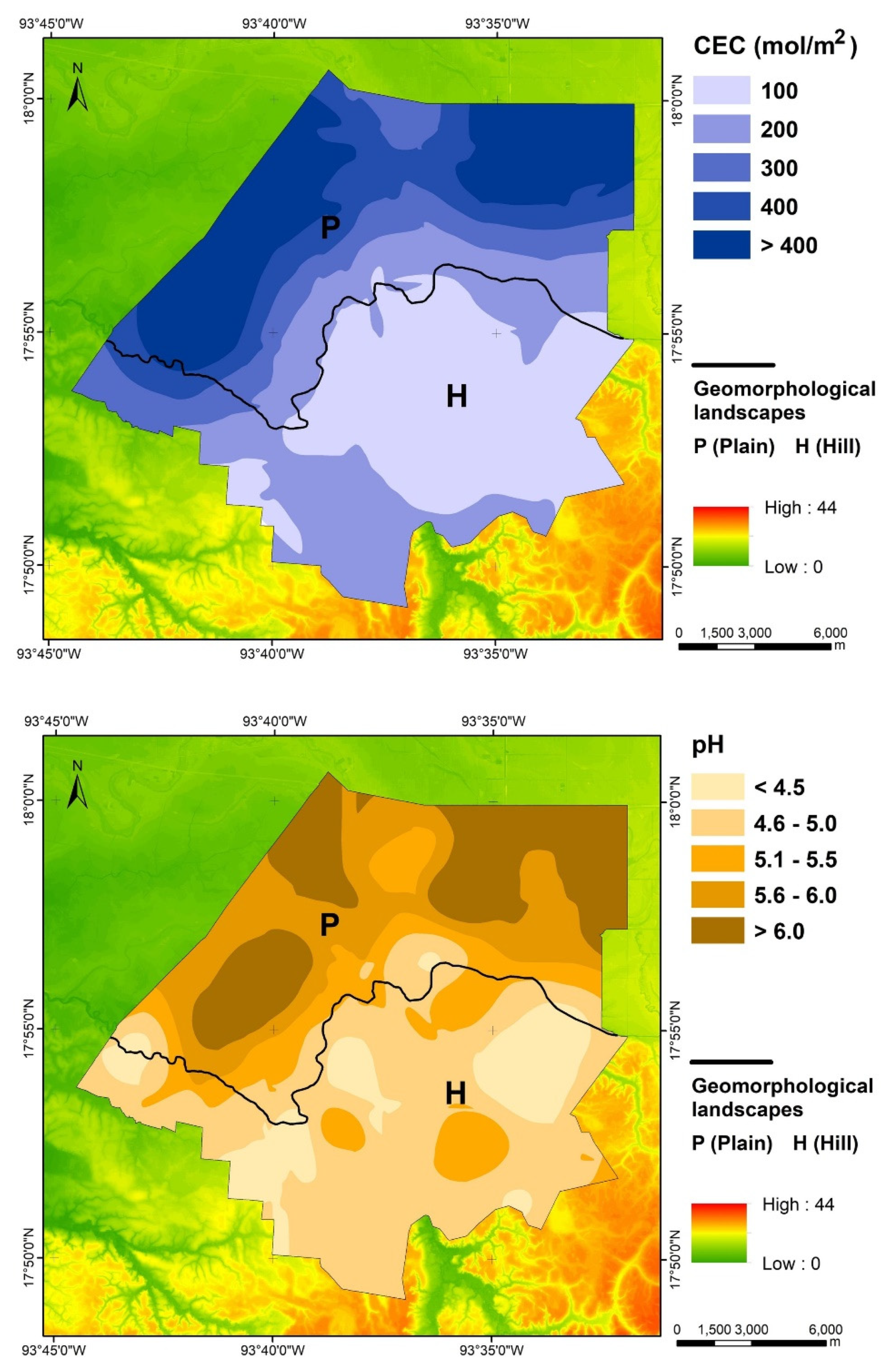
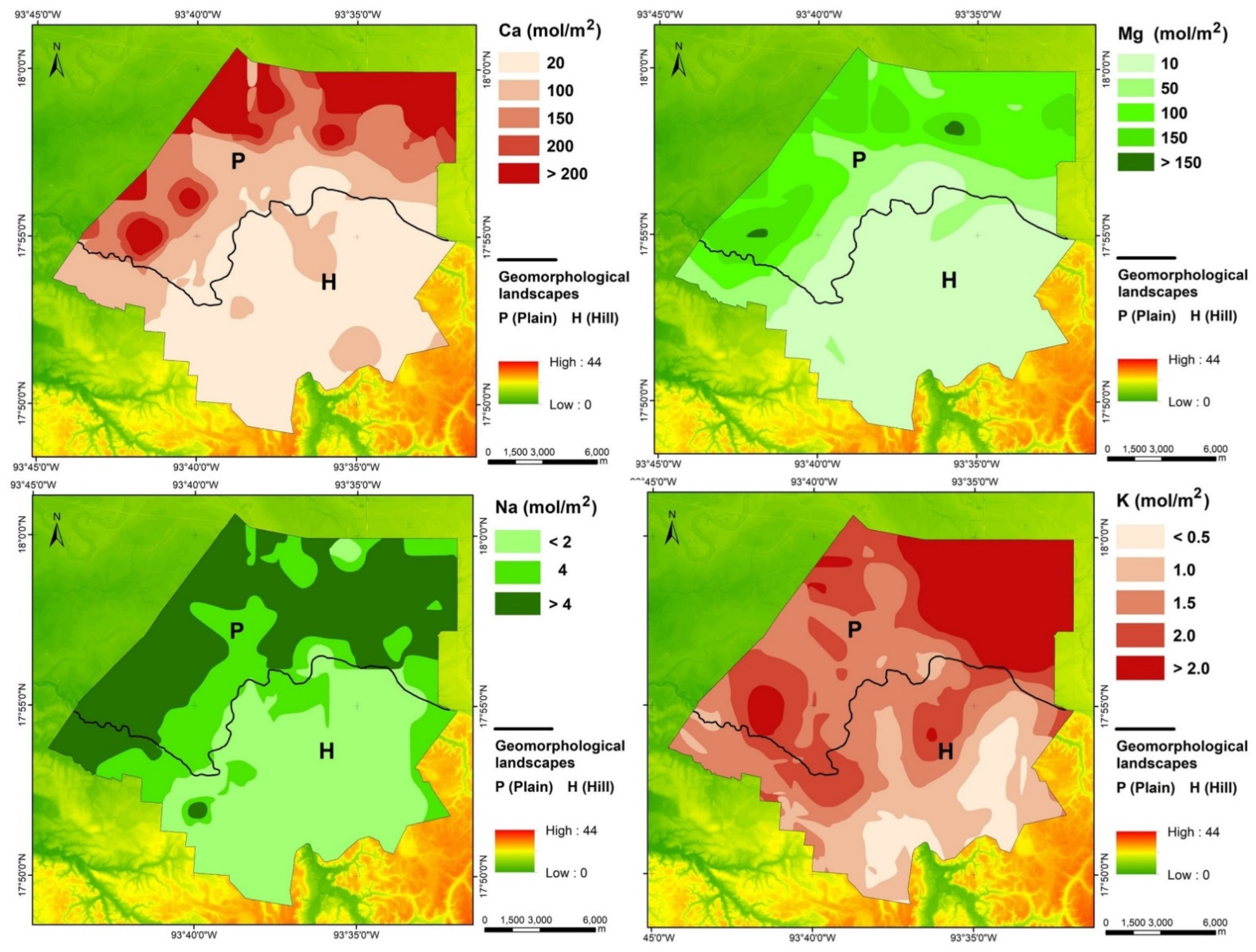
3. Results
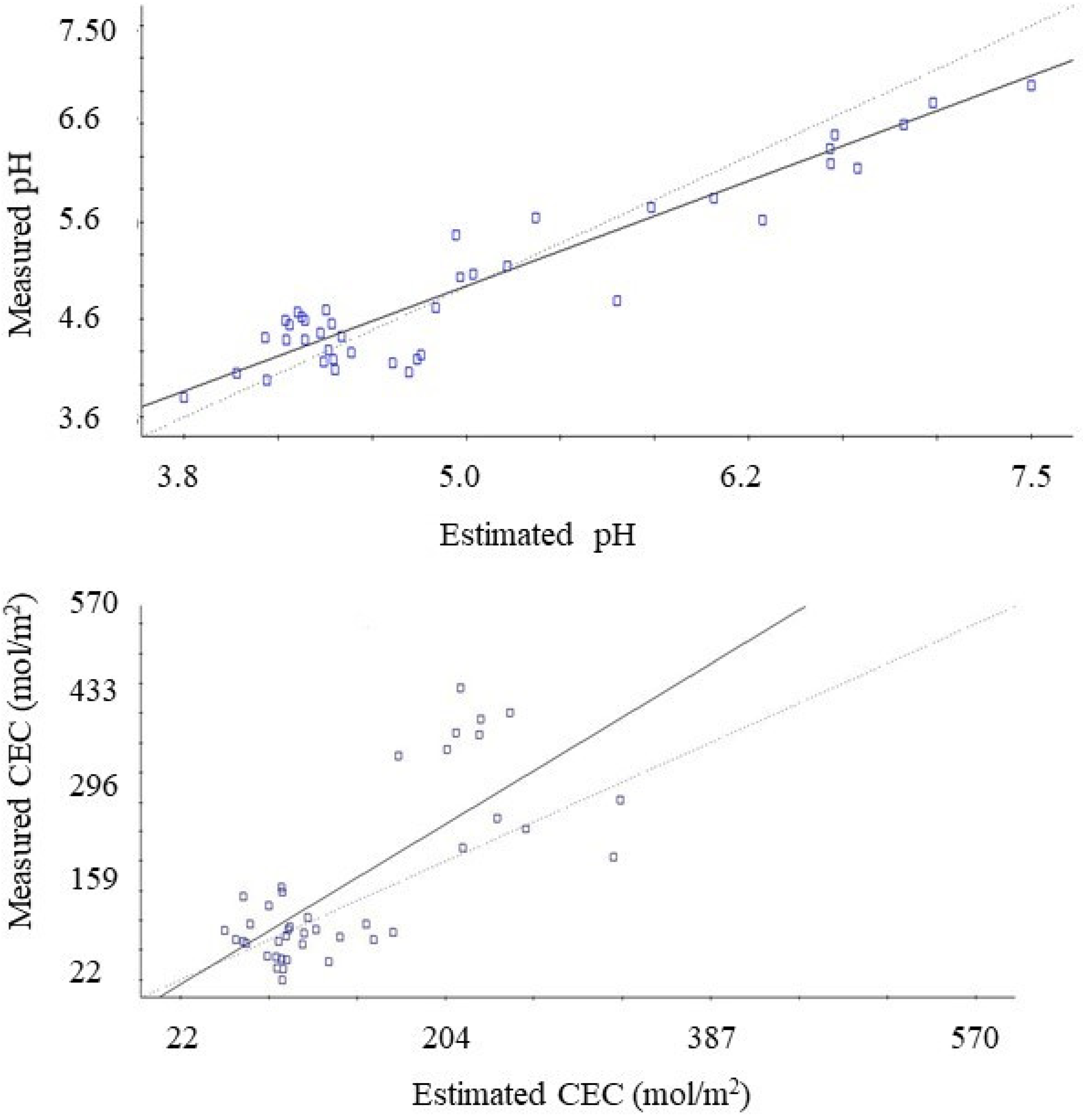
4. Discussion
4.1. Soils, Fertility, and Management
4.2. Method
5. Conclusions
Author Contributions
Funding
Institutional Review Board Statement
Informed Consent Statement
Acknowledgments
Conflicts of Interest
References
- Lajoie-O’Malley, A.; Bronson, K.; van der Burg, S.; Klerkx, L. The future(s) of digital agriculture and sustainable food systems: An analysis of high-level policy documents. Ecosyst. Serv. 2020, 45, 101183. [Google Scholar] [CrossRef]
- Molina-Maturano, J.; Verhulst, N.; Tur-Cardona, J.; Güereña, D.T.; Gardeazábal-Monsalve, A.; Govaerts, B.; Speelman, S. Understanding Smallholder Farmers’ Intention to Adopt Agricultural Apps: The Role of Mastery Approach and Innovation Hubs in Mexico. Agronomy 2021, 11, 194. [Google Scholar] [CrossRef]
- McBratney, A.B.; Santos, M.M.; Minasny, B. On Digital Soil Mapping. Geoderma 2003, 117, 3–52. [Google Scholar] [CrossRef]
- Minasny, B.; McBratney, A.B.; Malone, B.P.; Wheeler, I. Digital Mapping of Soil Carbon. Adv. Agron. 2013, 118, 1–47. [Google Scholar]
- Zinck, J.A. Geopedology: Elements of Geomorphology for Soil and Geohazard Studies; ITC-Faculty of Geo-Information Science and Earth Observation: Enschede, The Netherlands, 2013; 127p. [Google Scholar]
- Taghizadeh-Mehrjardi, R.; Sarmadian, F.; Minasny, B.; Triantafilis, J.; Omid, M. Digital Mapping of Soil Classes Using Decision Tree and Auxiliary Data in the Ardakan Region, Iran. Arid Land Res. Manag. 2014, 28, 147–168. [Google Scholar] [CrossRef]
- Alemán-Montes, B.; Búcaro-González, A.; Henríquez-Henríquez, C.; Largaespada-Zelaya, K. Mapeo Digital de Suelos Agrícolas En La Región Occidental Del Valle Central de Costa Rica. Agron. Costarric. 2019, 43, 157–166. [Google Scholar] [CrossRef]
- Bautista Zuñiga, F. Geostatistical Analysis of Soil Properties of the Karstic Sub-Horizontal Plain of the Yucatan Peninsula. Trop. Subtrop. Agroecosyst. 2021, 24, 1–11. [Google Scholar]
- Hernández, W.; Parra, L.M.M.; Rodríguez, D.G.T.; Romero, P. Variabilidad Espacial Del PH y Del Contenido de Fe2O3 En Suelos de La Cuenca Del Río Tabure Del Estado Lara. Rev. Cienc. Tecnol. 2018, 11, 19–27. [Google Scholar] [CrossRef]
- Zhang, G.; Liu, F.; Song, X. Recent Progress and Future Prospect of Digital Soil Mapping: A Review. J. Integr. Agric. 2017, 16, 2871–2885. [Google Scholar] [CrossRef]
- Lowenberg-DeBoer, J.; Erickson, B. Setting the Record Straight on Precision Agriculture Adoption. Agron. J. 2019, 111, 1552–1569. [Google Scholar] [CrossRef] [Green Version]
- Palma-López, D.J.; Vázquez, N.C.J.; Mata, Z.E.E.; López, C.A.; Morales, G.M.A.; Chable, P.R.; Contreras, H.J.; Palma-Cancino, D.Y. Zonificación de Ecosistemas y Agroecosistemas Susceptibles de Recibir Pagos Por Servicios Ambientales En La Chontalpa, Tabasco; Colegio de Postgraduados Campus Tabasco, Secretaría de Recursos Naturales y Protección Ambiental: Villahermosa, Mexico, 2011. [Google Scholar]
- Salgado-García, S.; Palma-López, D.J.; Zavala-Cruz, J.; Lagunes-Espinosa, L.C.; Castelán-Estrada, M.; Ortiz-García, C.F. Sistema Integrado Para Recomendar Dosis de Fertilizantes En Caña de Azúcar (SIRDF): Ingenio Presidente Benito Juárez; Colegio de Postgraduados, Campus Tabasco: Tabasco, Mexico, 2013. [Google Scholar]
- Aguilar-Rodríguez, J.R.; Zavala-Cruz, J.; Juárez-López, F.; Palma-López, D.J.; Castillo-Acosta, O.; Shirma-Torres, E. Aptitud Edáfica de Eucalyptus Urophylla ST Blake En La Terraza de Huimanguillo, Tabasco, México. Agro Product. 2017, 10, 79–85. [Google Scholar]
- Tinal-Ortiz, S.; López, D.J.P.; Zavala-Cruz, J.; Salgado-García, S.; Palma-Cancino, D.J.; Hidalgo-Moreno, C.I. Degradación química en Acrisoles bajo diferentes usos y pendientes en la sabana de Huimanguillo, Tabasco, México. Agro Product. 2020, 13. [Google Scholar] [CrossRef]
- Zavala Cruz, J.; Salgado García, S.; Marín Aguilar, Á.; Palma López, D.J.; Castelán Estrada, M.; Ramos Reyes, R. Transecto de suelos en terrazas con plantaciones de cítricos en Tabasco. Ecosistemas Recur. Agropecu. 2014, 1, 123–137. [Google Scholar]
- López-Castañeda, A.; Zavala-Cruz, J.; Palma-López, D.J.; Bautista-Zuñiga, F.; Rincón-Ramírez, J.A. Formas Del Terreno a Escala Detallada En Planicies y Lomeríos Del Municipio de Huimanguillo, Tabasco, México. Bol. Soc. Geológica Mex. 2022. en prensa. [Google Scholar]
- Salgado-García, S.; Palma-López, D.J.; Zavala-Cruz, J.; Ortiz García, C.F.; Castelán-Estrada, M.; Lagunes-Espinoza, L.C.; Guerrero-Peña, A.; Ortiz-Ceballos, A.L.; Córdova-Sánchez, S. Sistema Integrado Para Recomendar Dosis de Fertilizantes (SIRDF): En La Zona Piñera de Huimanguillo, Tabasco; Colegio de Postgraduados: Heroica Cárdenas, Mexico, 2010. [Google Scholar]
- Salgado García, S.; Palma López, D.J.; Zavala Cruz, J.; Ortiz García, C.F.; del Lagunés Espinoza, L.C.; Castelán Estrada, M.; Guerrero Peña, A.; Ortiz Ceballos, Á.I.; Córdova Sánchez, S. Integrated System for Recommending Fertilization Rates in Pineapple (Ananas comosus (L.) Merr.) Crop. Acta Agron. 2017, 66, 566–573. [Google Scholar] [CrossRef]
- Bautista, F.; Gallegos, A.; Pacheco, A. Análisis de las Funciones Ambientales de Los Suelos Con Datos de Perfiles (Soil & Environment); Skiu: Mexico City, Mexico, 2016; ISBN 978-607-96883-6-3. [Google Scholar]
- Гайегoс-Тавера, А.; Францискo, Б.; Дубрoвина, И.А. Soil & Environment Как Инструмент Для Оценки Экoлoгических Функций Пoчв. Прoграммные Прoдукты И Системы 2016, 114, 195–200. [Google Scholar] [CrossRef]
- Gallegos, Á.; López-Carmona, D.; Bautista, F. Quantitative Assessment of Environmental Soil Functions in Volcanic Zones from Mexico Using S&E Software. Sustainability 2019, 11, 4552. [Google Scholar] [CrossRef] [Green Version]
- Goovaerts, P. Geostatistical Modelling of Uncertainty in Soil Science. Geoderma 2001, 103, 3–26. [Google Scholar] [CrossRef]
- Delgado, C.; Pacheco, A.J.; Cabrera, S.A.; Batllori, S.E.; Orellana, R.; Bautista, F. Quality of groundwater for irrigation in tropical karst environment: The case of Yucatán, México. Agric. Water Manag. 2010, 97, 1423–1433. [Google Scholar] [CrossRef]
- Isaaks, E.H.; Srivastava, R.M. An Introduction to Applied Geostatistics; Department of Applied Earth Sciences; Oxford University Press: New York, NY, USA, 1990; ISBN 978-0-19-505013-4. [Google Scholar]
- Aceves-Navarro, L.A.; Rivera-Hernández, B. Clima. In La Biodiversidad en Tabasco. Estudio de Estado; Comisión Nacional para el Conocimiento y Uso de la Biodiversidad (CONABIO) y Gobierno del Estado de Tabasco: Tabasco, Mexico, 2019; Volume I, pp. 61–68. [Google Scholar]
- Servicio Geológico Mexicano (SGM). Carta Geológico-Minera Villahermosa E15-8 Tabasco, Veracruz, Chiapas y Oaxaca. Serv. Geológico Mex.; Servicio Geológico Mexicano (SGM): Pachuca, Mexico, 2005. [Google Scholar]
- Palma-López, D.J.; Moreno-Caliz, E.; Rincón-Ramírez, J.A.; Shirma, T.E. Degradación y Conservación de Los Suelos del Estado de Tabasco; Colegio de Postgraduados, CONACYT, CCYTET: Villahermosa, México, 2008. [Google Scholar]
- Cuanalo de la Cerda, H. Manual Para Descripción de Perfiles de Suelo En El Campo, 3rd ed.; Colegio de Postgraduados: Chapingo, Mexico, 1981. [Google Scholar]
- Mc Lean, E.O. Soil PH and Lime Requirement. In Methods of soil analysis—Part 2—Chemical and Microbiological Properties; Madison, W.I., Ed.; American Society of Agronomy Inc. and Soil Science Society of America: Estados Unidos, 1982; pp. 199–224. Available online: https://acsess.onlinelibrary.wiley.com/doi/abs/10.2134/agronmonogr9.2.2ed.c12 (accessed on 10 January 2022).
- USDA. Soil Survey Laboratory Methods Manual. Soil Survey Investigations Version 3.0; United State Department of Agriculture, Natural Resources Conservation Service, National Soil Survey Center: Washington, DC, USA, 1996; p. 693.
- Nelson, D.W.; Sommers, L.E. Total Carbon, Organic Carbon, and Organic Matter. Methods Soil Anal. Part 2 Chem. Microbiol. Prop. 1982, 9, 535–577. [Google Scholar]
- Okalebo, J.R.; Gathua, K.W.; Woomer, P.L. Laboratory Methods of Soil and Plant Analysis. A Working Manual; The Tropical Soil Biology and Fertility Programme; Regional Office for Science and Technology for Africa; Soil Chemistry Laboratory, the Kenya Agricultural Research Institute, National Agricultural Research Centre: Muguga, Kenya, 1993. [Google Scholar]
- Gandoy, B.W. Manual de Laboratorio Para El Manejo Físico de Suelos, Departamento de Suelos; Universidad Autónoma de Chapingo: Texcoco, Mexico, 1992; p. 111. [Google Scholar]
- Robertson, G.P. GS+: Geostatistics for the Environmental Sciences; GS+: Plainwell, MI, USA, 2008; Available online: https://www.scirp.org/(S(czeh2tfqyw2orz553k1w0r45))/reference/ReferencesPapers.aspx?ReferenceID=1500353 (accessed on 10 January 2022).
- Webster, R.; Oliver, M.A. Statistical Methods in Soil and Land Resource Survey; Oxford University Press: New York, NY, USA, 1990. [Google Scholar]
- Hernandez-Stefanoni, J.L.; Ponce-Hernandez, R. Mapping the Spatial Variability of Plant Diversity in a Tropical Forest: Comparison of Spatial Interpolation Methods. Environ. Monit. Assess. 2006, 117, 307–334. [Google Scholar] [CrossRef] [PubMed]
- ESRI. An Overview of the Spatial Statistics Toolbox; ESRI: Redlands, CA, USA, 2004. [Google Scholar]
- Bautista, F.; Durán-de-Bazúa, C.; Lozano, R. Cambios Químicos En El Suelo Por Aplicación de Materia Orgánica Soluble Tipo Vinazas. Rev. Int. Contam. Ambient. 2000, 16, 89–101. [Google Scholar]
- Gallegos-Tavera, Á.; Bautista, F.; Álvarez, O. Software Para La Evaluación de Las Funciones Ambientales de Los Suelos (Assofu). Rev. Chapingo Ser. Cienc. For. Ambiente 2014, 20, 237–249. [Google Scholar]
- Salgado-García, S.; Colorado, J.A.; Salgado-Velázquez, S.; Sánchez, S.C.; López, D.P.; Ramírez, J.A.R.; Castañeda, A.L. Spatial Variability of Some Chemical Properties of a Cambisol Soil with Cocoa (Theobroma cacao L.) Cultivation: Variabilidad Espacial. Agro Product. 2021, 14, 43–48. [Google Scholar] [CrossRef]
- Minasny, B.; McBratney, A. Digital soil mapping: A brief history and some lessons. Geoderma 2016, 264, 301–311. [Google Scholar] [CrossRef]
- Nagarjuna, N.R.; Chakraborty, P.; Roy, S.; Singh, K.; Minasny, B.; McBratney, A.; Biswas, A.; Das, B.S. Legacy data-based national-scale digital mapping of key soil properties in India. Geoderma 2021, 381, 114684. [Google Scholar] [CrossRef]


| Parameters | Mean | Skewness | Kurtosis | Minimal Value | Maximal Value | Standard Deviation |
|---|---|---|---|---|---|---|
| pH | 4.99 | 0.93 | −0.30 | 3.83 | 7.33 | 0.9 |
| EC (dS m−1) | 0.047 | 1.45 | 2.33 | 0.00 | 0.24 | 0.05 |
| COS (t ha−1) | 129.9 | 1.20 | 2.16 | 43.07 | 330.13 | 56.8 |
| P (mg kg−1) | 12.32 | 2.79 | 9.48 | 0.00 | 74.54 | 26.9 |
| Nt (%) | 0.175 | 1.07 | 2.97 | 0.01 | 0.58 | 0.11 |
| CEC (mol m−2) | 173.2 | 1.18 | 0.17 | 22.22 | 570.12 | 143.1 |
| Ca (mol m−2) | 78.4 | 1.41 | 0.83 | 0.40 | 407.67 | 112.8 |
| Mg (mol m−2) | 38.3 | 1.42 | 0.60 | 0.41 | 184.41 | 56.1 |
| K (mol m−2) | 1.4 | 0.86 | 0.11 | 0.02 | 4.65 | 1.1 |
| Na (mol m−2) | 2.3 | 3.04 | 11.45 | 0.01 | 18.36 | 3.3 |
| FC (L m−2) | 617.3 | −2.45 | 6.65 | 239.48 | 815.10 | 1.0 |
| Soil Properties | Model | Nugget | Sill | Range (m) | Model r2 |
|---|---|---|---|---|---|
| CEC (pH covariant) | Gaussian | 0.10 | 92 | 5520 | 0.80 |
| CEC (mol m−2) | Gaussian | 0.12 | 2.22 | 13590 | 0.86 |
| pH | Gaussian | 0.13 | 1.02 | 5530 | 0.87 |
| Ca (mol m−2) | Gaussian | 0.31 | 3.63 | 4160 | 0.96 |
| Mg (mol m−2) | Gaussian | 0.71 | 3.98 | 6310 | 0.90 |
| Na (mol m−2) | Gaussian | 0.01 | 18.54 | 2963 | 0.88 |
| K (mol m−2) | Gaussian | 0.67 | 2.02 | 5470 | 0.65 |
| P (mg kg−1) | Gaussian | 2.60 | 149.10 | 27.60 | 0.86 |
| EC (dS m−1) | Gaussian | 0.01 | 0.03 | 5890 | 0.80 |
| Nt (%) | Exponential | 0.01 | 0.04 | 30780 | 0.52 |
| SOC (t ha−1) | Linear | 0.18 | 0.18 | 13498 | 0.48 |
| FC (L m−2) | Gaussian | 0.03 | 0.15 | 7787 | 0.30 |
Publisher’s Note: MDPI stays neutral with regard to jurisdictional claims in published maps and institutional affiliations. |
© 2022 by the authors. Licensee MDPI, Basel, Switzerland. This article is an open access article distributed under the terms and conditions of the Creative Commons Attribution (CC BY) license (https://creativecommons.org/licenses/by/4.0/).
Share and Cite
López-Castañeda, A.; Zavala-Cruz, J.; Palma-López, D.J.; Rincón-Ramírez, J.A.; Bautista, F. Digital Mapping of Soil Profile Properties for Precision Agriculture in Developing Countries. Agronomy 2022, 12, 353. https://doi.org/10.3390/agronomy12020353
López-Castañeda A, Zavala-Cruz J, Palma-López DJ, Rincón-Ramírez JA, Bautista F. Digital Mapping of Soil Profile Properties for Precision Agriculture in Developing Countries. Agronomy. 2022; 12(2):353. https://doi.org/10.3390/agronomy12020353
Chicago/Turabian StyleLópez-Castañeda, Antonio, Joel Zavala-Cruz, David Jesús Palma-López, Joaquín Alberto Rincón-Ramírez, and Francisco Bautista. 2022. "Digital Mapping of Soil Profile Properties for Precision Agriculture in Developing Countries" Agronomy 12, no. 2: 353. https://doi.org/10.3390/agronomy12020353