Rapid Nondestructive Detection of Chlorophyll Content in Muskmelon Leaves under Different Light Quality Treatments

Abstract

In order to select the light quality suitable for plant growth, a quantitative detection model of chlorophyll content in muskmelon leaves was established to monitor plant growth quickly and accurately. In the paper, muskmelon “Boyang 91” was used as the experimental material, and six different light proportion treatments were set up. Through measuring plant height, stem diameter, number of leaves, nodes, and other growth indicators, in addition to leaf chlorophyll content, the response difference of muskmelon to different light qualities was explored in a plant factory. The hyperspectral imaging technology was used to establish the prediction model for the chlorophyll content of muskmelon. The original spectrum was preprocessed and optimized by five pretreatments, and then the characteristic wavelengths were extracted by six methods. Partial least squares regression (PLSR), least squares support vector machine (LSSVM), and convolutional neural network (CNN) were established for optimal feature wavelength. The results showed that the plant height and stem diameter of the T3 treatment were higher than those of other treatments, and their values were 14.48 (cm) and 5.02 (mm), respectively. The chlorophyll content of the T3 treatment was the highest, and its value was 40.16 (mg/g), which was higher than that of other treatments. Through comprehensive analysis, the T3 treatment (light ratio: 6R/1B/2W, light quantum flux: 360 μmol/(m²·s), photoperiod: 12 h) was optimal. Meanwhile, the average spectral reflectance data of 216 leaf samples were extracted, and the S-G preprocessing method was selected to preprocess the original spectral data (Rc = 0.860, RMSEC = 1.806; Rcv = 0.790, RMSECV = 2.161). By comparing and analyzing the correlation coefficients and root mean square errors of six feature wavelength extraction methods, it was concluded that the variable combination population analysis (VCPA) method had the best model effect for feature wavelength extraction (R_P = 0.824, RMSEP = 1.973). Ten characteristic wavelengths ( 396, 409, 457, 518, 532, 565, 687, 691, 701, and 705 nm) extracted by the VCPA method were used to establish the chlorophyll content prediction model, and the chlorophyll content prediction model of S-G-VCPA-CNN had the best performance (Rc = 0.9151, RMSEC = 1.445; Rp = 0.811, RMSEP = 2.055). The results of this study provide data support and a theoretical basis for screening the light ratio of other crops, and also present technical support for online monitoring of crop growth in plant factories.

1. Introduction

Muskmelon is an important economic and medicinal crop [1] and has a large planting area in Ningxia [2,3]. The chlorophyll content of crop leaves not only reflects the nutritional status and growth characteristics of plants, but also has a significant impact on crop yield and quality [4]. Therefore, real-time monitoring of chlorophyll content in crop leaves is conducive to accurate monitoring of crop nutrition and growth. Hyperspectral imaging can be employed to predict chlorophyll content in plants because of its fast, nondestructive, low-cost, and direct quantitative analysis of weak spectral differences in vegetation [5,6,7,8]. Feature wavelength extraction and model construction were the most important steps in hyperspectral imaging technology. Therefore, using the feature wavelength extraction method, including SPA, CARS, UVE, etc., combined with PLSR, BP neural network, etc., a prediction model has been established for hyperspectral data to predict chlorophyll concentration of peaches [9], rice [10], rape [11,12], green beans [13], potatoes [14], and winter wheat [15]. In the work of Du Minghua et al. [7], hyperspectral imaging technology was used to optimize the extraction method of UVE characteristic wavelength, and three prediction models of leaf chlorophyll content, namely PLSR, multiple linear regression (MLR), and principal component regression (PCR), were established. The results showed that the combination of UVE and the PLSR model was the best (Rp = 0.850, RMSEP = 4.338). In the study by Wang Xiaoyan et al. [16], SPA and CARS were to extract characteristic wavelengths to establish a PLSR prediction model for chlorophyll content in millet leaves at different growth stages. The results showed that SPA combined with the PLSR model had the best prediction effect for different growth periods. In the work of Yang Jing et al. [11], the BP neural network model was established using hyperspectral imaging technology to predict the chlorophyll content of rape leaves. The results show that the BP neural network model is stable, and its accuracy is greatly improved (R2 = 0.812, RMSE = 1.399). The above research results show that it is feasible to use hyperspectral imaging technology to establish characteristic wavelength extraction combined with a modeling method to detect chlorophyll content. Hyperspectral achievement technology has been extensively studied in the detection of chlorophyll content in other crops, but little research has been conducted in muskmelon, particularly the chlorophyll content of muskmelon leaves in plant factories.

In this study, we used the muskmelon “Boyang 91” as the experimental material and picked the leaves of muskmelon fruit stages through different light quality treatments in a plant factory. The specific objectives of this study were to (1) acquire the spectral responses in muskmelon leaves from hyperspectral images using the visible near-infrared hyperspectral imaging system (400~1000 nm), (2) build a quantifiable relationship between spectral data and measured chlorophyll content values using chemometrics techniques, (3) obtain the informative wavelengths using a variable selection technique, (4) develop a chlorophyll content prediction model with the selected wavelength bands, and (5) evaluate the performance of the developed prediction model in terms of robustness and accuracy.

2. Materials and Methods

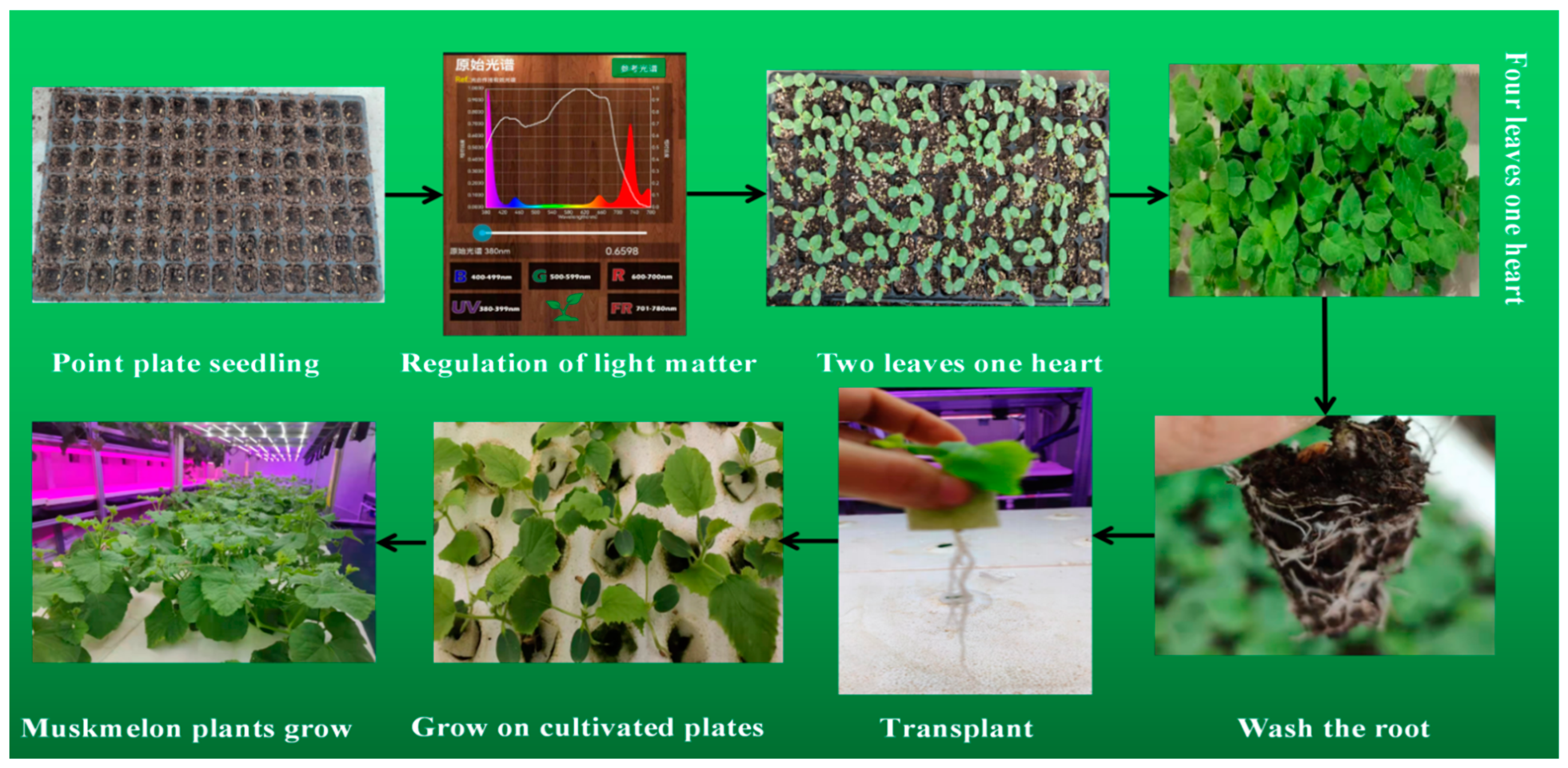
2.1. Experimental Materials

The muskmelon variety “Boyang 91” was purchased from Ningxia Borui Agricultural Technology Co. The variety is a thin-skinned muskmelon, a new hybrid variety, with strong plant growth, resistance to powdery mildew and fusarium wilt, strong fruit setting ability, and good taste.

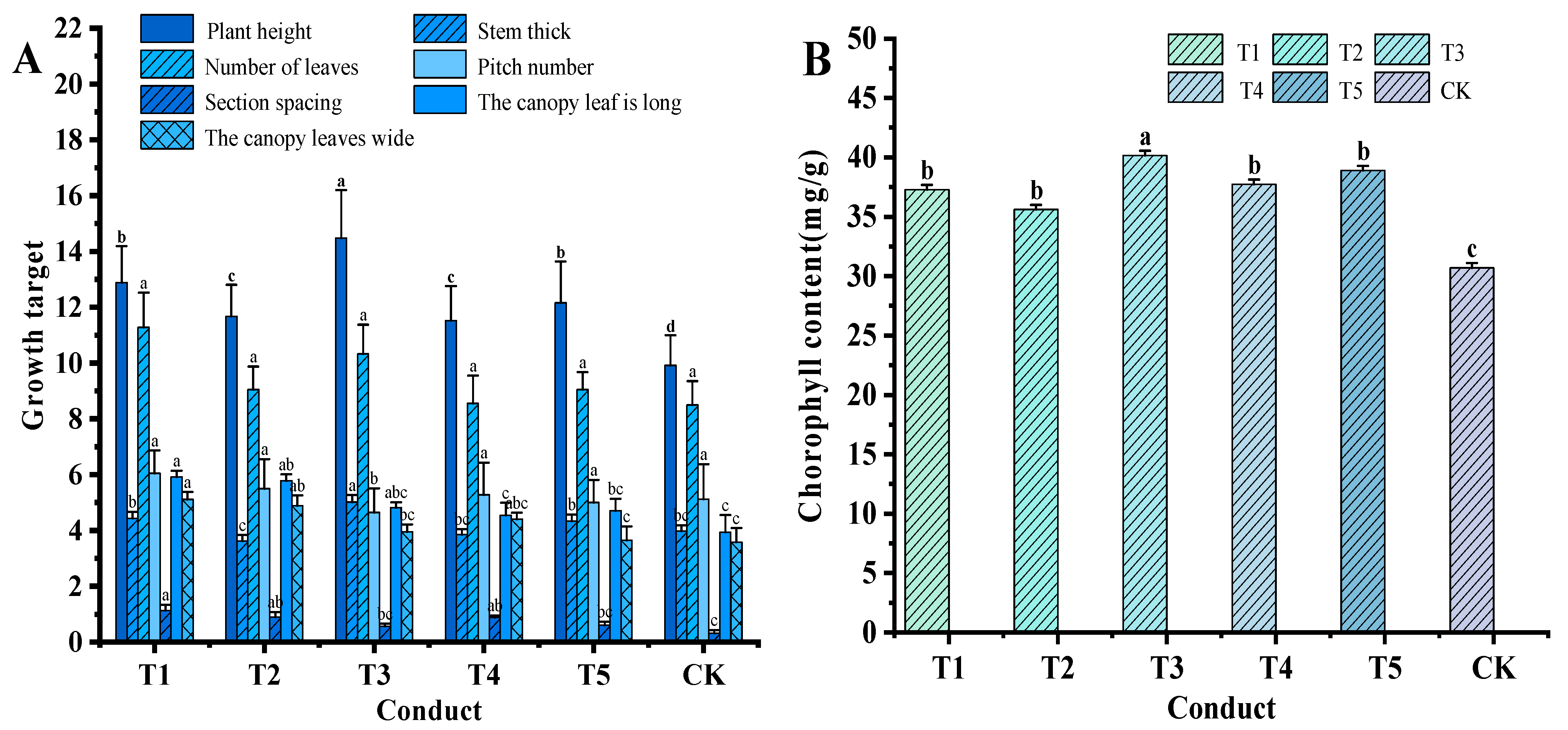
2.2. Experimental Design

The experiment was carried out in the plant factory of Ningxia Horticultural Industrial Park from March 2022 to June 2022 (geographic location: 35°14′~39°23′ N, 104°17′~107°39′ E; temperature: 26~35 °C in daytime, 14~18 °C at night; humidity: 65~75%; CO₂ concentration: 400~1200 ppm, covering an area of 225 m²). The size of the controlled environmental room is 40 m². The plant was planted with nutrient solution (garden trial formula, pH value: 6.5~7.0, EC value: 2~3 mS/cm) and a 98-point tray was used for seedlings (seedling cultivation in plant factory cultivation room). During seedling cultivation, the light quality of the plant factory was regulated (first, the light was placed 20 cm away from the LED light plate, and the parameters of red light, blue light, white light, ultraviolet light, and far-red light were adjusted until the light intensity reached the specified value). When the muskmelon seedlings grew to the four-leaf center, they were transplanted to the planting plate of the plant factory. The substrate of the seedling root was cleaned off with clean water, then the stem was wrapped with a sponge, the root was dipped in water, and finally the root was immersed in 2/3 of the nutrient solution. Each treatment had 30 seedlings. The process of muskmelon from sowing to growth and development is shown in Figure 1. The muskmelon seedlings were treated with different light ratios, as shown in

Table 1. Design of muskmelon growth and development. R/B/W represents red light, blue light, and white light.

Handle	Light Ratio	Light Quantum Flux (μmol/(m2·s))	Photoperiod (h)
T1	3R/2B/3W	360	12
T2	8R/4B/5W/2FR/1UVa
T3	6R/1B/2W
T4	4R/3B/2W/1FR
T5	7R/3B/5W/1UVa
CK	White light

. After planting, the growth indicators ( using ruler, tape measure, and vernier caliper) and chlorophyll content (using SPAD-502Plus, Konica Minolta) were measured every 7 days. A total of 216 canopy leaf samples were collected during the muskmelon fruiting stage. To minimize chlorophyll loss, spectral collection and chlorophyll quantification were carried out immediately after picking [17].

2.3. Spectral Data Acquisition

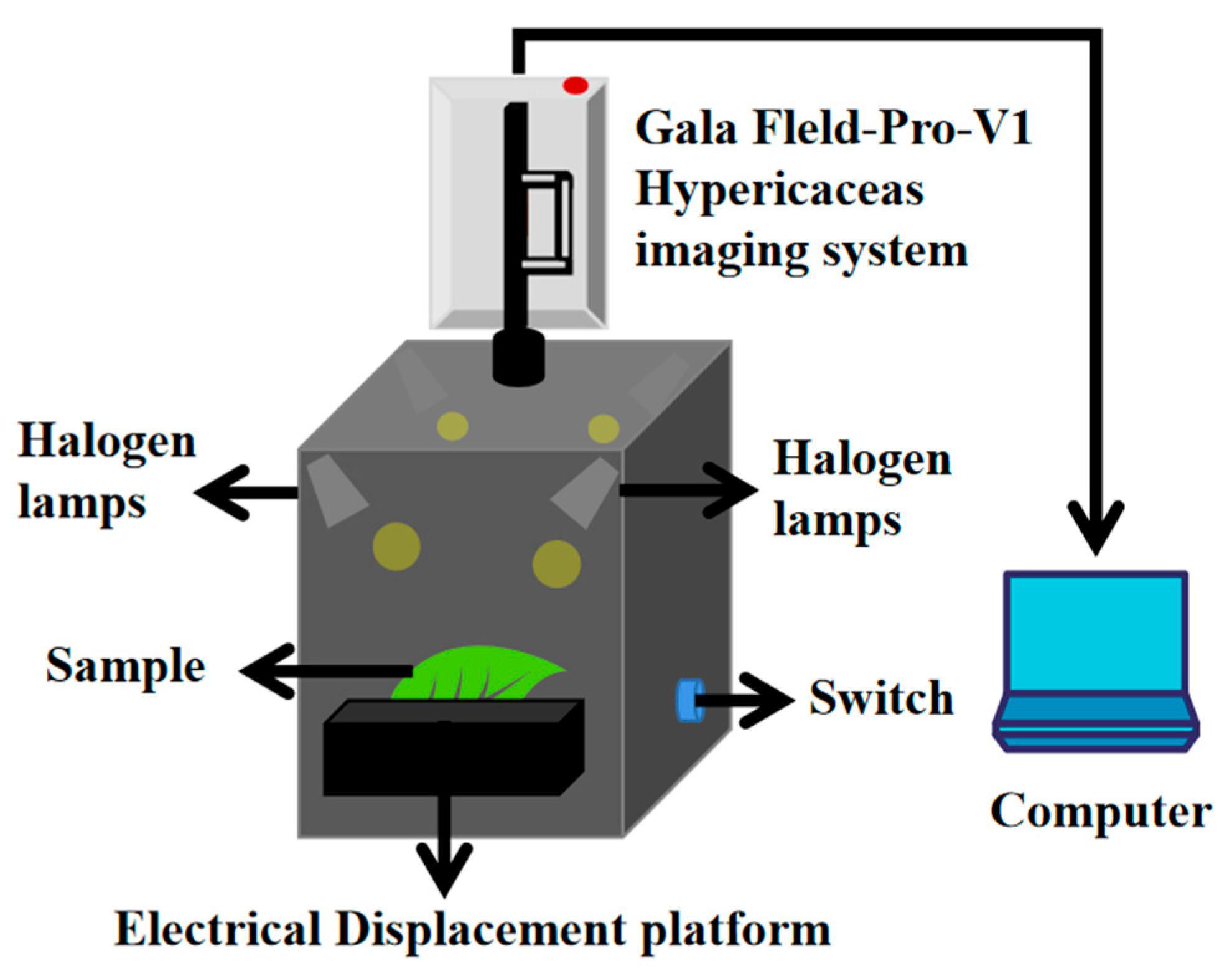
2.3.1. Hyperspectral Imaging Equipment and Image Calibration

We conducted hyperspectral scanning in the Spectral Laboratory of the School of Food and Wine, Ningxia University. Figure 2 shows the hyperspectral imaging system. The visible near-infrared band hyperspectral imaging system (400~1000 nm) contains GaiaField-F-V10, produced by Sichuan Shuangli Hepu Co., Ltd. (Beijing China), and has 175 bands with a spectral resolution of 3.8 nm. Because the shape and color of the blade cause diffuse reflection of the light source, a reasonable displacement platform speed and exposure time were set.

Each sample was placed on a black background and scanned. The final acquisition parameters were determined after the pre-experiment: object distance was 300 mm, scanning speed was set to 0.147 cm/s, imaging spectrometer exposure time was 13 ms, and gain was set to 1. In order to eliminate image noise and uneven distribution of light source intensity, the obtained hyperspectral images needed to be corrected in black and white. Under the equipment environment consistent with the sample measurement, the whiteboard image was first obtained through the standard black and white correction plate, then the camera lens was covered, and the acquisition control background was selected. Then, the camera measured the blackboard image. Black and white correction is shown in Equation (1):

$$R=\frac{T_{raw}-T_{dark}}{T_{white}-T_{dark}}$$

(1)

where T_raw is the original image, T_dark is the blackboard correction image, T_white is the correction image, and R is the corrected hyperspectral image.

2.3.2. Region of Interest Selection and Sample Division

The region of interest of the collected spectral image was extracted by ENVI 5.3 software. Six regions of interest (ROI), avoiding the vein, were selected from the leaves as the mean spectra of the leaves. A total of 216 sample sets were obtained. The random sample (RS) method was used to divide the samples, in which 2/3 (144) were used as the calibration set and 1/3 (72) was used as the prediction set, calculated according to a 2:1 ratio. The formula is shown in (2).

Suppose (x₁, x₂, ..., x_n) is a simple random sample from President X, and its one observation value is (x₁, x₂, ... x_n,), x₍₁₎ < x₍₂₎ < ... < x_(n), where the frequency of x_(i) (i = 1, 2, ..., r) is n_i (n₁ + n₂ + ... + n_r = n):

$$\mathrm{Fn}\left(\mathrm{x}\right)=\left\{\begin{array}{c}0, x<x\left(1\right)\\ \frac{n1+n2+...+nk}{n} (x\left(k\right)<x\le x\left(k+1\right)\\ 1, x\ge x\left(r\right)\end{array}\right.$$

(2)

2.4. Spectral Data Analysis

2.4.1. Spectral Data Preprocessing

Spectral preprocessing methods have the purpose of reducing the limitation of spectral curves due to instrument noise, dark current, multicollinearity, and background influence factors [18,19]. In this study, the original spectrum was pretreated with Gaussian filtering, Savitzky–Golay (S-G), multiple scattering correction (MSC), Detrending, standard normal variate transformation (SNV), etc., through Unscrambler X 10.4, and the optimal pretreatment method based on chlorophyll content samples was selected by combining the comparative analysis of PLSR model performance parameters.

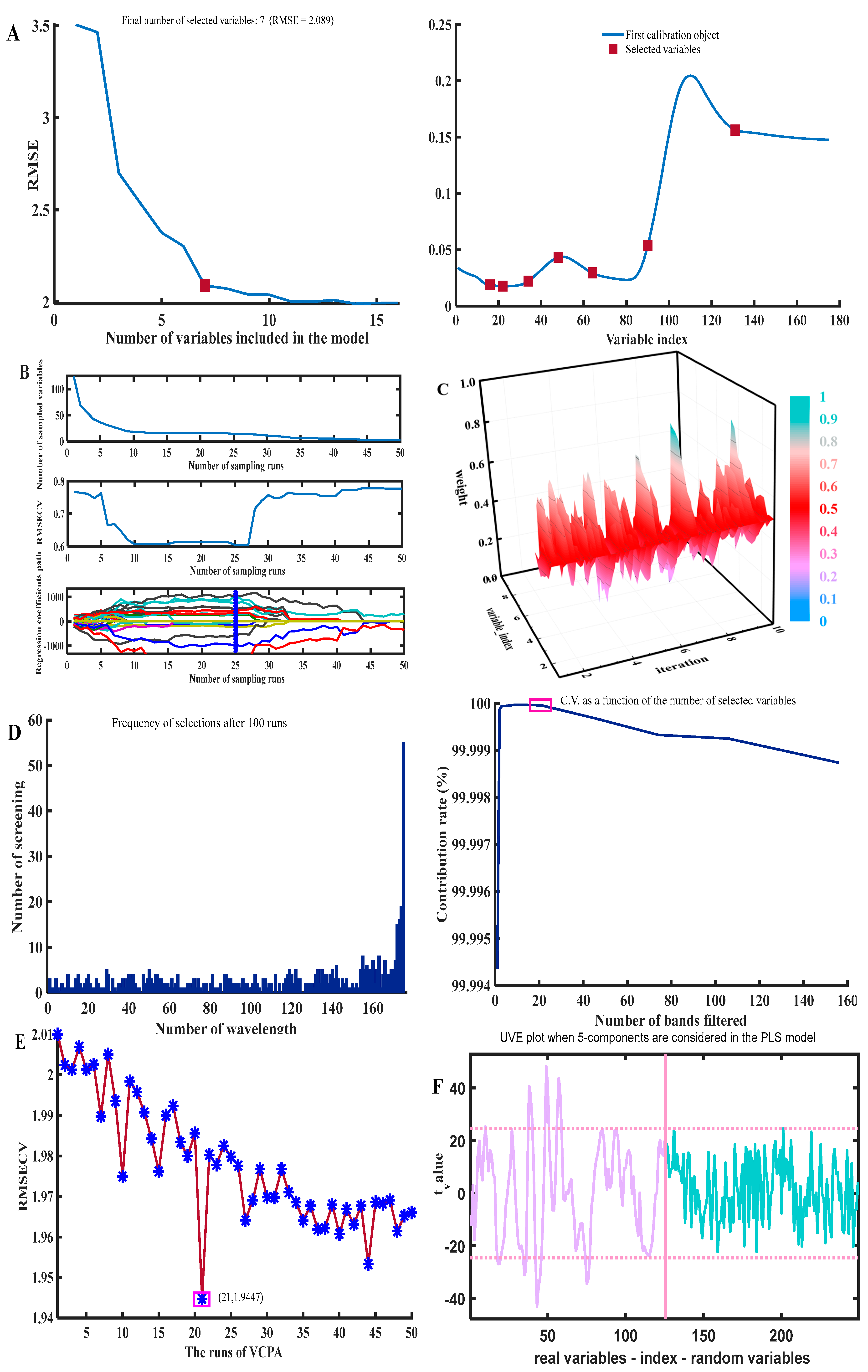
2.4.2. Extraction of Characteristic Wavelengths

Spectral imaging technology can produce a large number of wavelengths, a large number of data points, and redundant information. In order to improve the performance of the classification model, the original spectral data were reduced by extracting effective information and reducing the number of model operations [20]. In this study, the characteristic wavelengths of the successive projections algorithm (SPA), competitive adaptive reweighted sampling (CARS), interval variable iterative space shrinking analysis (iVISSA), genetic algorithm and partial least squares (GAPLS), variable combination population analysis (VCPA), and uninformation variable elimination (UVE) were extracted by MATLAB 2020a software to establish the PLSR prediction model. The BMS sampling strategy adopted by VCPA provided the same sampling probability for each variable. It compressed the variable space through EDF, eliminated irrelevant variables, and used the MPA idea to retain the first 10% of the optimal subset of variables. The probability of important variables being finally selected was relatively high, so there were few variables ultimately retained [21].

2.4.3. Model Building and Evaluation

The quantitative analysis models are commonly used in molecular spectroscopy combined with thermometric methods, including linear and nonlinear. In this experiment, PLSR, LSSVM, and CNN models were built by Unscrambler X 10.4 and MATLAB 2020a software. The evaluation indicators were RMSEC and Rc² in the training set and RMSEP and Rp² in the prediction set, where RMSE was the prediction error indicator, and R² was the determination coefficient indicator. Therefore, a better prediction model is expected to have a lower RMSE and a higher R². The specific formula is as follows:

$$R^2=\frac{{\displaystyle \sum _i^n{({\widehat{y}}_i-y_i)}^2}}{{\displaystyle \sum _i^n{({\widehat{y}}_i-y_m)}^2}}$$

(3)

$$RMSECV=\sqrt{\frac{{\displaystyle \sum _{i=1}^n{({\widehat{y}}_i-y_i)}^2}}{n-1}}$$

(4)

$$RMSEP=\sqrt{\frac{{\displaystyle \sum _{i=1}^n{({\widehat{y}}_i-y_i)}^2}}{m-1}}$$

(5)

where y_i is the measured value of the ith sample, ${\widehat{y}}_i$ is the predicted value of the ith sample, y_m is the average of the measured results of each data set, n is the number of corrected samples, and m is the number of samples in the test set.

3. Results

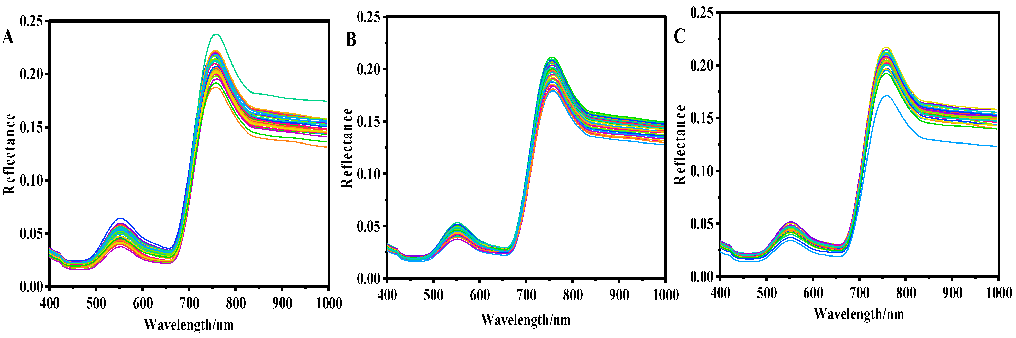
3.1. Spectral Data Acquisition

The spectral information of muskmelon leaves was extracted by Envi 5.3 software, and the original spectral curves of chlorophyll content of leaves under six different light ratios were obtained, as shown in Figure 3.

It can be seen from Figure 3 that the change trend of the spectral curve of leaf chlorophyll content under six different light quality treatments was basically consistent, and there was an obvious change rule. There were two absorption valleys at 495 nm and 660 nm in the range of blue light (434~502 nm) and red light (602~687 nm), which were mainly due to the absorption of chlorophyll in leaves; there was a reflection “green peak” at 551 nm in the green light band (512~558 nm). In the 701–800 nm spectral band region, the reflection spectrum curve increased rapidly, showing a steep and nearly vertical feature, resulting in the “red edge” phenomenon [18]. In the near-infrared region, the spectral reflectance of muskmelon leaves was a high reflection region, which was controlled by the internal cell structure of muskmelon leaves. By comparing the leaf reflectivity of different chlorophyll contents, it can be seen that the reflectivity of muskmelon leaves was different with different chlorophyll contents. With the increase in chlorophyll content, the reflectivity decreased gradually in the visible light range and increased gradually in the near-infrared area. On the whole, in the visible light and near-infrared ranges (400~1000 nm), except 705~736 nm, the spectral reflectance curves of muskmelon with different chlorophyll contents change obviously, which was easy to distinguish [22]. As the spectrum collected included the absorption of other substances in addition to chlorophyll, it was necessary to analyze the spectral data and establish a prediction model with a high correlation of chlorophyll through chemometric methods. A portable chlorophyll analyzer (SPAD-502Plus, Konica Minolta) was used to determine the chlorophyll content. The measurement time was between 9:00 and 11:00 in the morning. Three leaves of each plant, free from pests and diseases, physiological spots, and mechanical damage, were selected, and the SPAD values were measured directly with a chlorophyll meter. Three points were measured per leaf and averaged, and the chlorophyll values were recorded for a total of 216 samples. The SPSS 20.0 soft program (version 20.0; IBM Corp., Armonk, NY, USA) was used to analyze the single-factor variance of muskmelon growth indicators and leaf chlorophyll content under six different light quality treatments (T1, T2, T3, T4, T5, and CK). The strip chart of muskmelon growth indicators and leaf chlorophyll content was drawn by Origin software. The results are shown in Figure 4.

It can be seen from Figure 4A that plant height, stem diameter, and node number of muskmelon under the T3 treatment are significantly different from those of other treatments. There was a significant difference between pitch and CK, but no significant difference between pitch and T1, T2, T4, and T5. There was no significant difference in leaf number, canopy leaf length, and canopy leaf width between T3 and other treatments. It can be seen from Figure 4B that the chlorophyll content of muskmelon leaves under CK treatment was significantly different from other treatments, and its value was the lowest compared with other treatments. The difference in chlorophyll content in muskmelon leaves under T1, T2, T4, and T5 treatments was not obvious, but there was a significant difference between the chlorophyll content in the T3 treatment and the other five treatments, with a value of 40.16 (mg/g). Therefore, the T3 treatment was preferred for later tests under the other fixed condition parameters in the plant factory.

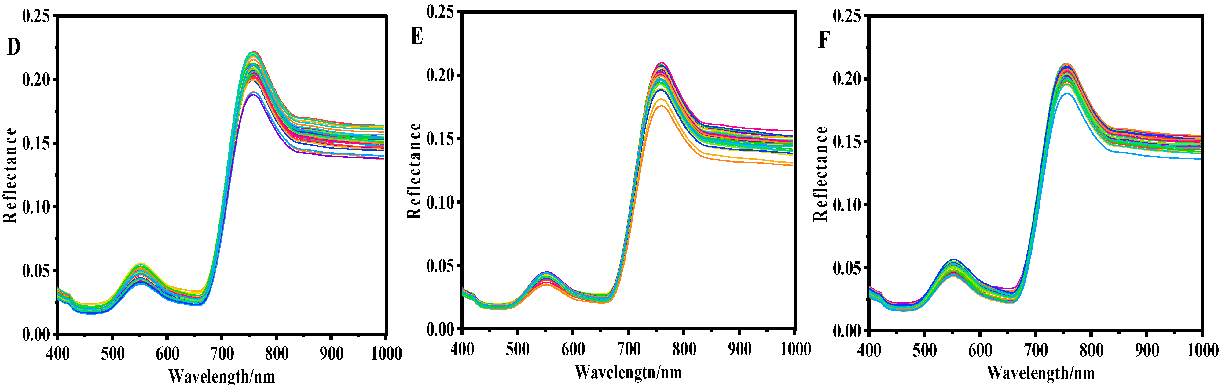
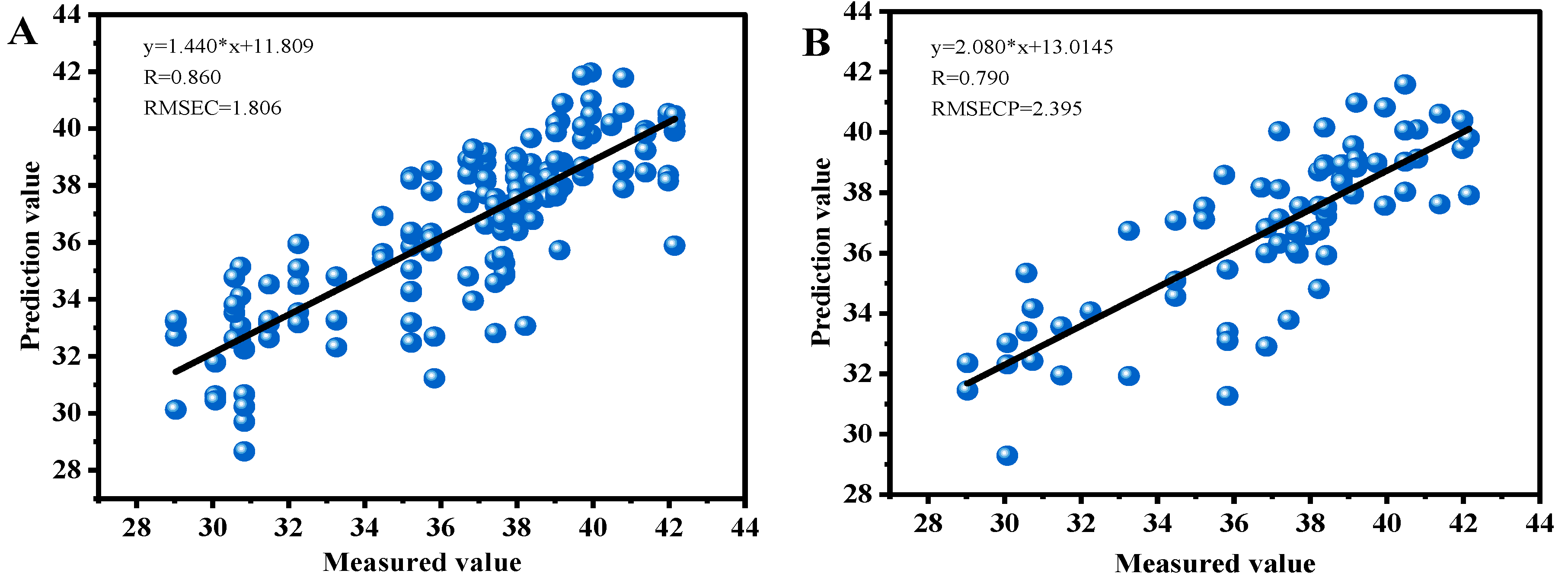
3.2. Analysis of Pretreatment Effect

Since hyperspectral images were 3D data with redundant information, and the original spectrum has baseline drift, it was necessary to preprocess the original spectrum to provide a basis for model construction. Spectral preprocessing methods have the purpose of reducing the limitation of spectral curves due to instrument noise, dark current, multicollinearity, and background influence factors [18,19]. The main preprocessing methods were Gaussian filtering, S-G, MSC, Detrending, and SNV. The optimal preprocessing method based on chlorophyll content samples was selected by comparing and analyzing the performance parameters of the PLSR model. The effects of different preprocessing modeling of chlorophyll content spectral data are shown in

Table 2. PLSR model statistics for different pretreatment methods of chlorophyll content.

Type	PCs	Rc	RMSEC (mg/g)	Rcv	RMSECV (mg/g)	Rp	RMSEP (mg/g)
Raw	12	0.847	1.881	0.786	2.205	0.807	2.056
Gaussian Filter	6	0.823	2.012	0.794	2.154	0.807	2.056
S-G	15	0.860	1.806	0.790	2.161	0.790	2.395
MSC	11	0.835	1.948	0.758	2.333	0.790	2.144
SNV	6	0.819	2.029	0.779	2.225	0.819	2.029
Detrending	13	0.857	1.824	0.750	2.388	0.776	2.221

.

As shown in Table 2, PLSR models of five different algorithms were used for preprocessing based on the original spectrum. Compared with the original spectral results, the R_C values after Gaussian filtering, MSC, and SNV processing decreased, and the modeling effect decreased to a certain extent: the minimum value was 0.819. However, the R_C values increased, and the model performance improved after S-G and Detrending pretreatment. The correlation coefficient of the calibration set obtained by the S-G preprocessing method was higher than that of the original spectrum and other preprocessing spectra, and R_C was 0.860. The correlation coefficient of the prediction set was higher than that of the Detrending preprocessing spectrum, and the R_P and RMSEC values were 0.790 and 1.806, respectively. Through comprehensive analysis, the S-G pretreatment method was optimized to establish the PLSR model. Figure 5A shows the effect of PLSR combined with S-G preprocessing for the calibration set, and Figure 5B shows the effect of PLSR combined with S-G preprocessing for the prediction set. Therefore, S-G can be selected to process the later data of muskmelon leaves.

3.3. Modeling Based on Characteristic Wavelengths

3.3.1. Feature Wavelength Extraction

In order to reduce the amount of data processing, it was necessary to apply some chemometric algorithms to extract the characteristic wavelength of data through Unscrambler 10.4 and MATLAB 2014a software. This method can not only effectively reduce a lot of useless information, but also improve the prediction ability and stability of the model. Six feature wavelength extraction methods, SPA, CARS, iVISSA, GAPLS, VCPA, and UVE, were used to eliminate redundant and noisy wavelengths (Figure 6). Figure 6 shows the running process of the selection of feature wavelengths by six methods.

When the SPA algorithm was used to filter characteristic wavelengths, the minimum number of wavelength variables included in the model was set to 7 and the maximum number was set to 20, and the RMSE value of 2.090 was calculated under different numbers of variables. Characteristic wavelength points were mainly distributed near the peaks, troughs, and turning points of the reflectivity curve. Seven characteristic wavelengths were extracted, as shown in Figure 6A. Figure 6B shows the process of the CARS algorithm screening feature variables in the 400~1000 nm band. The number of Monte Carlo samples was 50. At the 25th sampling, the RMSECV was the smallest, indicating that the wavelength variables unrelated to the chlorophyll content have been removed in the first 24 samples, while the key variables related to the chlorophyll content may be removed in the last 26 samples [20]. The RMSECV can obtain 17 feature bands at the minimum, as shown in Figure 6B. The iterations of the iVISSA algorithm and the variation in the sampling weight values of each wavelength with the number of iterations are shown in Figure 6C. The weight coefficients of each wavelength point remained essentially constant after fifteen times of iteration and the optimal wavelength subset was obtained. Sixty-four bands were extracted using iVISSA methods. When using the GAPLS algorithm to extract the characteristic wavelengths related to the chlorophyll content spectrum, the relevant parameters need to be debugged repeatedly. Through multiple experiments, the parameters were set as the following: population was 30; crossing probability was 50%; probability of variation was 1%; maximum genetic factor was 30; and iterations was 100 (as shown in Figure 6D). The BMS sampling strategy adopted by VCPA provided the same sampling probability for each variable. It compressed the variable space through EDF, eliminated irrelevant variables, and used the MPA idea to retain the first 10% of the optimal subset of variables. The probability of important variables being finally selected was relatively high, so there were few variables ultimately retained [21]. It can be seen from Figure 6E that when the number of samples was 21, RMSECV drops to 1.940. The 10 characteristic wavelengths screened by the VCPA method were 396, 409, 457, 518, 532, 565, 687, 691, 701, and 705 nm, respectively. It can be seen from Figure 6F that when the main component of the chlorophyll content in the muskmelon leaves determined by the UVE algorithm was 5 in the band of 400~1000 nm, the t-value value model had the best fitting effect, and finally 18 characteristic wavelengths were selected.

3.3.2. PLSR model of Characteristic Wavelengths

Table 3. PLSR models at different characteristic wavelengths of chlorophyll content.

Type	PCs	RC	RMSEC (mg/g)	RCV	RMSECV (mg/g)	RP	RMSEP (mg/g)
SPA	7	0.826	1.991	0.804	2.103	0.789	2.154
CARS	8	0.821	2.020	0.794	2.152	0.797	2.108
VCPA	9	0.844	1.897	0.817	2.045	0.824	1.973
UVE	8	0.755	2.321	0.707	2.510	0.700	2.671
GAPLS	5	0.703	2.931	0.793	2.995	0.760	2.671
iVISSA	9	0.840	1.918	0.800	2.119	0.813	2.125

shows the application of the PLSR method to build a correlation model for the characteristic wavelengths screened by different methods, and the results of the analysis are shown in Table 3.

It can be seen from Table 3 that the characteristic wavelengths were extracted by SPA, CARS, VCPA, UVE, GAPLS, and iVISSA algorithms. Compared with other characteristic wavelength extraction methods, the correlation coefficient of the PLSR model of chlorophyll content built by VCPA was higher than that of other algorithms (Rc = 0.844, R_CV = 0.817, R_P = 0.824), and the root mean square error of the PLSR model of chlorophyll content built by VCPA was lower than that of other algorithms (RMSEC = 1.897, RMSECV = 2.045, RMSEP = 1.973). In the comprehensive analysis, the model constructed by the VCPA method had the best effectiveness. The quantitative prediction model of chlorophyll content in muskmelon leaves was established by using the characteristic wavelength extracted by the optimized VCPA method (Figure 7). Figure 7A shows the correction set prediction model established by S-G in combination with the VCPA method. It can be seen from Figure 7A that the model fitting effect was good (y = 1.396*x + 10.546, Rc = 0.844, RMSEC = 1.897). Figure 7B shows the prediction set prediction model established by S-G in combination with the VCPA method. It can be seen from Figure 7B that the model fitting effect was good (y = 2.062*x + 12.320, Rp = 0.824, RMSEP = 1.973).

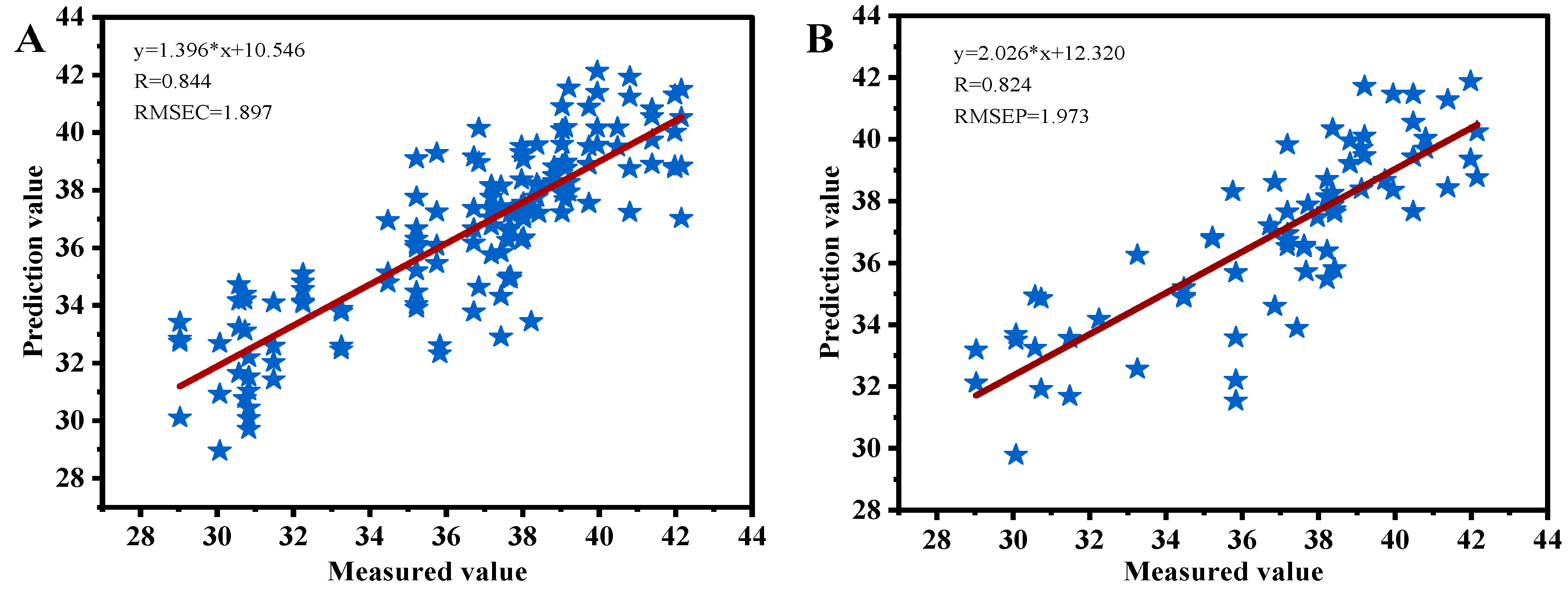
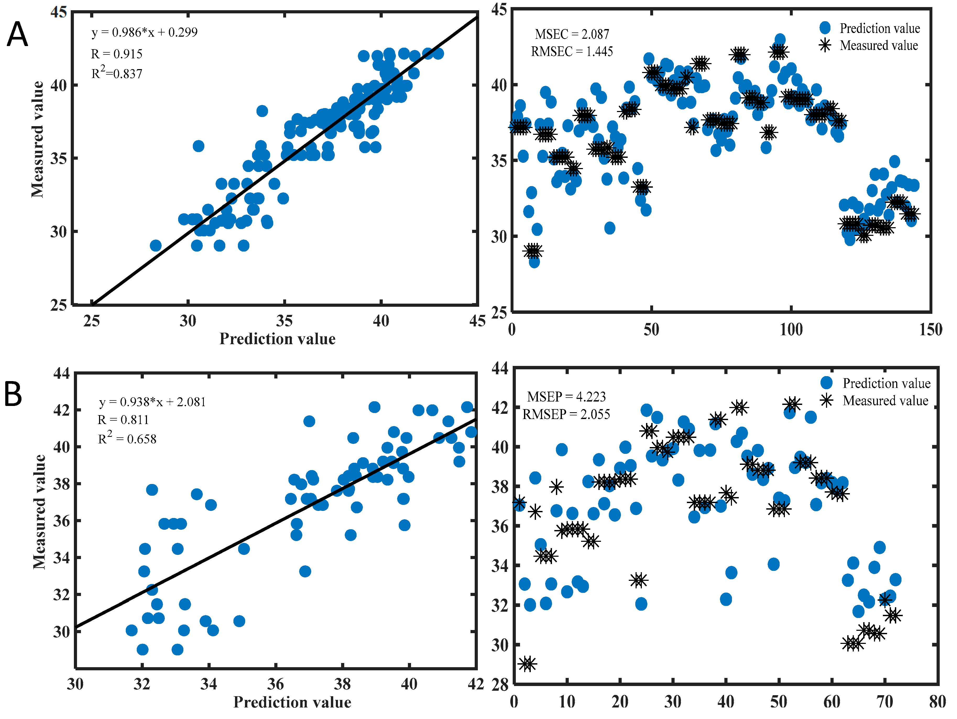
3.4. Comparative Analysis of Different Building Models

In the experiment, PLSR, LSSVM, and CNN models were utilized to construct the corresponding model for the wavelength extracted by the VCPA method. The results are presented in

Table 4. Comparative analysis of different modeling methods.

Spectral Feature Extraction Method	RC	RMSEC (mg/g)	RP	RMSEP (mg/g)
PLSR	0.844	1.897	0.824	1.973
LSSVM	0.819	1.997	0.799	2.214
CNN	0.915	1.445	0.811	2.055

.

It can be seen from Table 4 that the correlation coefficient RC of the model established by CNN was higher than that of PLSR and LSSVM, and its value was 0.915. The RP of the CNN model was higher than that of LSSVM: its value was 0.811. The RMSEC was lower than in the PLSR and LSSVM modeling methods, with a value of 1.445, and RMSEP was lower than in LSSVM, with a value of 2.055. According to a comprehensive analysis, CNN was the best model among the three modeling methods. Therefore, CNN was selected to establish a prediction model of chlorophyll content in muskmelon leaves (Figure 8). Figure 8A shows the correction set prediction model established by VCPA in combination with the CNN method. It can be seen from Figure 8A that the model fitting effect was good (y = 0.986*x + 0.299, Rc = 0.915, RMSEC = 1.445). Figure 8B showed the prediction set prediction model established by VCPA in combination with the CNN method. It can be seen from Figure 8B that the model fitting effect was good (y = 0.938*x + 2.081, Rp = 0.811, RMSEP = 2.055).

4. Discussion

The study found that the addition of an appropriate red and blue light ratio on the basis of white light in the T3 treatment was conducive to the healthy growth of muskmelon and increased chlorophyll content. It may be that the red light with the wavelength of 602~687 nm and the blue light with the wavelength of 434~502 nm were the main spectra for photosynthesis and photomorphogenesis of plants, which enhance photosynthesis and promote chlorophyll accumulation. Scholars also conducted relevant experiments in Chinese cabbage [23], peppers [24], watermelon [25], and other crops, and found that the appropriate ratio of red and blue light can promote the growth and development of crops, which was consistent with the results of this experiment. However, there were certain differences in the appropriate ratio of red and blue light for each crop, and there were also certain differences between the optimal ratio of light for muskmelon selected in this study and other crops. This shows that the demand for red light and blue light of plants varies with species.

The correlation coefficient values after Gaussian filtering, MSC, and SNV processing decreased, and the modeling effect decreased to a certain extent: the minimum value was 0.819, as shown in Table 2. This was because the three preprocessing methods of Gaussian filtering, MSC, and SNV can smooth the noise while smoothing the useful information, leading to spectral signal distortion and reducing the spectral modeling effect after preprocessing [26,27]. After S-G and Detrending preprocessing, the correlation coefficient increased and the model performance improved. Convolution smoothing can eliminate noise and minimize the impact of smoothing on useful information, thus optimizing the performance of the model [28]. The Detrending algorithm can eliminate the baseline drift of diffuse reflection, thus ensuring the stability and accuracy of the numerical value [27]. In this paper, S-G pretreatment had the best effect. Scholars preferred MSC [7] and SNV [11] pretreatment methods to predict the original spectra of chlorophyll content in tomato leaves and potato leaves, respectively, indicating that not all the original spectrum numbers were suitable for optimizing S-G pretreatment.

In terms of feature wavelength extraction, we found that the model constructed by the VCPA method had the best effect by comparing the correlation coefficient and root mean square error of six feature wavelengths extracted based on S-G in Table 3. Because the BMS sampling strategy adopted by VCPA provided the same sampling probability for each variable, the variable space was compressed through EDF to eliminate irrelevant variables, and the MPA idea was adopted to retain the top 10% optimal variable subset, so the probability of important variables being finally selected is relatively high [21]. The VCPA feature wavelength extraction method was first confirmed by Yun et al. [29]. Currently, the VCPA method and its combination with other modeling methods are widely used in food quality detection [30] and crop protein content [31]. In this paper, VCPA was used to set the sampling times: k was 1000; iterations N was 50; proportion of excellent subsets in k variable quantum sets σ was 10%; and the percentage of sampling times of each variable in the binary sampling matrix M in the total sampling times α was 0.1. A total of 10 characteristic wavelengths were extracted. In the study of Zhao Huai et al. [31], parameters were set through VCPA: K was 500, N was 50, σ was 10%, and α was 0.5. Finally, 14 characteristic bands were extracted.

In terms of modeling methods, we established PLSR, LSSVM, and CNN models based on VCPA, and concluded that CNN was the best model among the three modeling methods in Table 4. The reason may be that CNN is a deep learning model or a multilayer perceptron similar to an artificial neural network [32]. It is usually used for visual effect image detection and can learn training features from large drainage matrix data information and extend its results to the same type of unknown data information. The total amount of parameters required for calculation was greatly reduced, and the reduction in accuracy was effectively prevented. This was confirmed in the research of Yu et al. [33]. The researchers used CNN to estimate the fresh weight of lettuce and found that CNN had low demand for hardware and hundreds of original samples can be expanded to obtain better estimation accuracy. After fine-tuning, migration, and learning on the new task data set, the model achieved good results on the test set, but the model parameters were too large, and the training and prediction took a long time [32]. In this experiment, it was found that CNN was the best model to predict chlorophyll content, but the model parameters were small, there were certain limitations, and generalization ability and model stability were low.

A CNN is a multilayer feedforward neural network with convolution operation [32]. The core of CNN is convolution. There are convolution cores in the convolution layer of CNN. After the original image passes through the input layer, it will become grayscale or a matrix filled with RGB values. The convolution core and the image matrix are used to multiply and add the numbers in the corresponding convolution core, and then the data obtained will be filled into a new matrix (convolution). The convolution core moves on the image at a certain distance (step size). The new matrix can reflect some features (feature map) of the image: they are the output of the current layer and the input of the next layer. Setting different convolution kernels can find various features (training them). In addition to the convolution layer, CNN has two other important accessories: a pooling layer and full connection layer. The pooling layer can select the main features of the image. The commonly used max pooling method is the maximum value of the reserved window coverage area. After the matrix is pooled, the parameters will be greatly reduced. The full connection layer can gather the extracted features at the end of the network.

5. Conclusions

In this study, hyperspectral imaging technology was applied to nondestructive detection of chlorophyll content in muskmelon leaves under different light quality treatments in a plant factory. The T3 treatment (light ratio: 6R/1B/2W, light quantum flux: 360 μmol/(m²·s), photoperiod: 12 h) had a better performance in plant height, stem diameter, number of nodes, and leaf chlorophyll content of muskmelon plants. The prediction model of chlorophyll content in muskmelon leaves was established by fusion of spectral data. The calibration set and prediction set of 216 muskmelon leaf samples were divided by the RS method. The pretreatment method of S-G (R_C = 0.860, RMSEC = 1.806; R_P = 0.790, RMSECV = 2.395) was the best among the different pretreatment methods. The chlorophyll content prediction models were established by characteristic wavelengths extracted by SPA, CARS, iVISSA, GAPLS, VCPA, and UVE, and the 10 characteristic wavelengths (396, 409, 457, 518, 532, 565, 687, 691, 701, and 705 nm) extracted by VCPA method had the best model effect (R_P = 0.824, RMSEP = 1.973). Compared with PCR and LSSVM models, the S-G-VCPA-CNN model had the best performance in leaf chlorophyll content (R_C = 0.915, R_P = 0.811). The S-G-VCPA-CNN prediction model of chlorophyll content in muskmelon leaves based on hyperspectral imaging technology provided a reference for rapid detection of other indicators of muskmelon plants and also provided technical support for online monitoring of crop growth in plant factories.

The structure of the CNN model used in this study was fixed, and the generalization ability and stability of the model were low. In the later stage, the generalization ability and stability of the chlorophyll content prediction model can be improved by expanding the number of samples. In addition, this study cannot achieve real-time monitoring of the chlorophyll content of muskmelon leaves. In future, more kinds of algorithms can be explored, and more accurate and stable models can be used to carried out the development of online monitoring equipment for the chlorophyll content of other plants.

References

1. Zheng, J.; Hu, M.J.; Guo, Y.P. Regulation of plant photosynthesis by photosynthesis and its mechanism. J. Appl. Eco. 2008, 19, 1619–1624. [Google Scholar] [CrossRef]
2. Yang, N.; Wang, W.Y.; Cao, C.Y.; Wu, J.X. Analysis of the development status and trend of melon Industry in China. Chin. Melon Veg. 2019, 32, 50–54. [Google Scholar] [CrossRef]
3. Du, H.Y.; Liu, S.F.; Guo, S.; Yu, R.; Wang, Z.Q.; Guo, S.J.; Tian, M.; Dong, R. Ningxia West melon industry technology development status and right Policy Research. North. Hortic. 2013, 19, 177–179. [Google Scholar]
4. Tian, R.C.; Gao, Z.Q.; Zhou, K. SPAD value estimation of late indica rice varieties based on hyperspectral data. CLJ 2021, 27, 45–50. [Google Scholar] [CrossRef]
5. Liu, W.Y.; Pan, J. Neural network-based model for high spectral estimation of chlorophyll content. J. Appl. Eco. 2017, 28, 1128–1136. [Google Scholar] [CrossRef]
6. Li, C.C.; Shi, J.J.; Ma, C.Y.; Cui, Y.Q.; Wang, Y.L.; Li, Y.C. Estimation of chlorophyll content in winter wheat based on wavelet transform and fractional differentiation. J. Agric. Mach. 2021, 52, 172–182. [Google Scholar] [CrossRef]
7. Du, M.H.; Yang, T.; Ma, Y.; Zhang, J.; Wu, L.G. Detection of chlorophyll content in tomato leaves based on NIR hyperspectral imaging technology. JAAS. 2022, 50, 48–55. [Google Scholar] [CrossRef]
8. Meng, L.; Zhang, J.; Yang, T.; Wu, L.G. Study on the visual distribution of chlorophyll content in tomato leaves based on hyperspectral imaging technology. Hubei Agric. Sci. 2022, 61, 171–177. [Google Scholar] [CrossRef]
9. Sun, Y.; Wang, Y.H.; Xiao, H.; Gu, X.Z.; Pan, L.Q.; Tu, K. Hyperspectral imaging detection of decayed honey peaches based on their chlorophyll content. Food Chem. 2017, 235, 194–202. [Google Scholar] [CrossRef]
10. Kang, L.; Gao, R.; Kong, Q.M.; Jia, Y.J.; Shi, Y.B.; Su, Z.B. Hyperspectral imaging estimation of SPAD values in rice leaves. J. Northeast Agric. Univ. 2020, 51, 89–96. [Google Scholar] [CrossRef]
11. Yang, J. Monitoring Model of Chlorophyll Content in Rapeseed Leaves Based on Hyperspectral Imaging Technology. Master–s Thesis, Hunan Agricultural University, Changsha, China, 2020. [Google Scholar]
12. Xia, J.A.; Cao, H.X.; Yang, Y.W.; Zhang, W.X.; Wan, Q.; Xu, L.; Ge, D.K.; Zhang, W.Y.; Ke, Y.Q.; Huang, B. Detection of waterlogging stress based on hypersensitive images of oilseed rape leaves (Brassica lupus L.). Comput. Electron. Agric. 2019, 159, 59–68. [Google Scholar] [CrossRef]
13. Madeira, A.C.; Mentions, A.; Ferreira, M.E.; Taborda, M.L. Relationship between spectrora diometric and chlorophyll measurements in green beans. Commun. Soil Sci. Plant Anal. 2000, 31, 631–643. [Google Scholar] [CrossRef]
14. Zhuo, W.; Yu, X.F.; Li, X.T.; Gong, D.D.; Feng, J. Hyperspectral imaging technology enables chlorophyll NT detection in potato leaves. Opt. Instrum. 2020, 42, 1–8. [Google Scholar] [CrossRef]
15. Wang, W.; Peng, Y.K.; Ma, W.; Huang, H.; Wang, X. High Spectroscopic detection technology of chlorophyll content in winter wheat. J. Agric. Mach. 2010, 41, 172–177. [Google Scholar] [CrossRef]
16. Wang, X.Y. Methods on Chlorophyll Content Prediction and Variety Identification in Millet. Ph.D. Thesis, Shanxi Agricultural University, Taigu, China, 2019. [Google Scholar] [CrossRef]
17. Ma, L.; Xia, J.F.; Zhan, F. Effects of Spectral Pretreatment on Nondestructive Evaluation of Soluble Solids Content of Tomatoes with near Infrared Spectroscopy. J. Agric. Eng. 2009, 25, 350–354. [Google Scholar] [CrossRef]
18. Li, S.L. Visualization of chlorophyll distribution in soybean leaves based on hyperspectral imaging. Guizhou Agric. Sci. 2022, 50, 41–50. [Google Scholar] [CrossRef]
19. Shang, J.; Zhang, Y.; Meng, Q.L. Non-destructive identification of apple varieties by visible/NIR spectroscopy. Fresh Process. 2019, 19, 8–14. [Google Scholar]
20. Zheng, K.; Feng, T.; Zhang, W.; Huang, X.W.; Li, Z.H.; Zhang, D.; Yao, Y.; Zou, X.B. Variable selection by double competitive adaptive reweighted sampling for calibration transfer of near infrared spectra. Chemom. Intell. Lab. Syst. 2019, 191, 109–117. [Google Scholar] [CrossRef]
21. Wang, H.Y.; Song, J.; Pan, L.Q.; Yuan, P.S.; Guo, Z.H.; Xu, H.L. Optimizing the BP neural network to improve the accuracy of detecting the total number of colonies in conditioned chicken meat. J Agr Sci. 2020, 36, 302–309. [Google Scholar] [CrossRef]
22. Wang, F.D.; Yan, Z.Y.; Zhao, X.M.; Guo, X.; Zhou, Y.; Guo, J.X. Partial least squares model parameter selection. J. Jiangxi Agric. Univ. 2022, 44, 86–96. [Google Scholar] [CrossRef]
23. Chen, Y.W.; Liu, S.Q.; Cheng, B.; Liu, Q.; Ma, G.Q. Effects of different LED light sources on Chinese cabbage growth and quality. J. Chang. Veg. 2013, 16, 36–40. [Google Scholar] [CrossRef]
24. Yorio, N.C.; Goins, G.D.; Kagie, H.R.; Wheeler, R.M.; Sager, J.C. Improving spinach, radish, and lettuce growth under red light-emitting diodes (LEDs) with blue light supplementation. HortScience 2001, 36, 380–383. [Google Scholar] [CrossRef] [PubMed] [Green Version]
25. Bantis, F.; Koukounaras, A.; Siomos, A.S.; Fotelli, M.N.; Kintzonidis, D. Bichromatic red and blue LEDs during healing enhance the vegetative growth and quality of grafted watermelon seedlings. Sci. Hortic. 2019, 261, 109000. [Google Scholar] [CrossRef]
26. Rinnan, Å.; Berg, F.V.D.; Engelsen, S.B. Review of the most common pre-processing techniques for near-infrared spectra. TrAC Trends Anal. Chem. 2009, 28, 1201–1222. [Google Scholar] [CrossRef]
27. Barnes, R.J.; Dhanoa, M.S.; Lister, S.J. Correction to the Description of Standard Normal Variate (SNV) and De-Trend (DT) Transformations in Practical Spectroscopy with Applications in Food and Beverage Analysis-2nd Edition. J. Near Infrared Spec. 1993, 1, 185–186. [Google Scholar] [CrossRef]
28. Chen, L.P.; Yu, F.Q.H.; Tao, R.; Chen, G.D.; Li, S.J.; Xue, C.G. Prediction of moisture content during oyster dry processing based on hyperspectral imaging techniques. Chin. J. Food Prod. 2020, 20, 261–268. [Google Scholar] [CrossRef]
29. Yun, Y.H.; Wang, W.T.; Deng, B.C.; Lai, G.B.; Liu, X.B.; Ren, D.B.; Liang, Y.Z.; Fan, W.; Xu, Q.S. Using variable combination population analysis for variable selection in multivariate calibration. Anal. Chim. Acta 2015, 862, 14–23. [Google Scholar] [CrossRef]
30. Zhang, F.J.; Shi, L.; Li, L.X.; Zhao, H.R.; Zhu, Y.L. Nondestructive identification of Panax notoginseng powder quality grade for hyperspectral imaging. Spectrosc. Spectr. Anal. 2022, 42, 2255–2261. [Google Scholar] [CrossRef]
31. Zhao, H.; Huan, K.W.; Zheng, F.; Shi, X.G. Study on variable selection in near-infrared spectrum of wheat protein based on variable combination cluster analysis. Spectrosc. Spectr. Anal. 2016, 35, 51–54. [Google Scholar] [CrossRef]
32. Gai, R.L.; Cai, J.R.; Wang, S.Y.; Cang, Y.; Chen, N. A Review of the Application of Convolutional Neural Networks in Image Recognition. Small Microcomput. Syst. 2021, 42, 1980–1984. [Google Scholar]
33. Yu, C.C.; Wang, X.; Wu, J.Z.; Liu, Q. Hyperspectral detection of imperfect wheat grains based on a CNN neural network. Food Sci. 2017, 38, 283–287. [Google Scholar] [CrossRef]
Figure 1. Flow diagram of muskmelon planting in the plant factory.
Agronomy 12 03223 g001
Figure 2. The hyperspectral imaging system.
Agronomy 12 03223 g002
Figure 3. Raw spectra of chlorophyll content of muskmelon leaves under different light matter treatments. (AF) The raw spectrum of chlorophyll content of muskmelon leaves under different light treatments: A—T1; B—T2; C—T3; D—T4; E—T5; and F—CK.
Agronomy 12 03223 g003aAgronomy 12 03223 g003b
Figure 4. Chlorophyll content and growth index of muskmelon leaves under different light matter treatment. (A) is the growth indicator; (B) is the chlorophyll content. Different lowercase letters indicate significant differences in the growth index and chlorophyll content between different treatments in the same period (p < 0.05).
Agronomy 12 03223 g004
Figure 5. PLSR combined with S-G preprocessing modeling. (A) shows the effect of PLSR combined with S-G preprocessing for the calibration set, and (B) shows the effect of PLSR combined with S-G preprocessing for the prediction set.
Agronomy 12 03223 g005
Figure 6. The running process of the selection of feature wavelengths: (A) is SPA; (B) is CARS; (C) is iVISSA; (D) is GAPLS; (E) is VCPA; (F) is UVE.
Agronomy 12 03223 g006
Figure 7. PLSR prediction model of chlorophyll content based on VCPA characteristic wavelength extraction methods: (A) is calibration set; (B) is prediction set.
Agronomy 12 03223 g007
Figure 8. The performance of S-G-VCPA-CNN model: (A) is calibration set; (B) is prediction set.
Agronomy 12 03223 g008