A New Framework for Winter Wheat Yield Prediction Integrating Deep Learning and Bayesian Optimization

Abstract

Early prediction of winter wheat yield at the regional scale is essential for food policy making and food security, especially in the context of population growth and climate change. Agricultural big data and artificial intelligence (AI) are key technologies for smart agriculture, bringing cost-effective solutions to the agricultural sector. Deep learning-based crop yield forecast has currently emerged as one of the key methods for guiding agricultural production. In this study, we proposed a Bayesian optimization-based long- and short-term memory model (BO-LSTM) to construct a multi-source data fusion-driven crop growth feature extraction algorithm for winter wheat yield prediction. The yield prediction performance of BO-LSTM, support vector machine (SVM), and least absolute shrinkage and selection operator (Lasso) was then compared with multi-source data as input variables. The results showed that effective deep learning hyperparameter optimization is made possible by Bayesian optimization. The BO-LSTM (RMSE = 177.84 kg/ha, R² = 0.82) model had the highest accuracy of yield prediction with the input combination of “GPP + Climate + LAI + VIs”. BO-LSTM and SVM (RMSE = 185.7 kg/ha, R² = 0.80) methods outperformed linear regression Lasso (RMSE = 214.5 kg/ha, R² = 0.76) for winter wheat yield estimation. There were also differences between machine learning and deep learning, BO-LSTM outperformed SVM. indicating that the BO-LSTM model was more effective at capturing data correlations. In order to further verify the robustness of the BO-LSTM method, we explored the performance estimation performance of BO-LSTM in different regions. The results demonstrated that the BO-LSTM model could obtain higher estimation accuracy in regions with concentrated distribution of winter wheat cultivation and less influence of human factors. The approach used in this study can be expected to forecast crop yields, both in regions with a deficit of data and globally; it can also simply and effectively forecast winter wheat yields in a timely way utilizing publicly available multi-source data.

1. Introduction

Wheat is one of the top three crops in the world and is an important source of calories, protein, and many micronutrients for humans [1,2]. However, there are many constraints in production that pose serious threats to the stable and high yield potential of wheat, for example, increased temperature, increased precipitation variability, and frequent extreme events [3,4]. Therefore, early prediction of crop yield before harvest is of great value for our food security and trade.

Traditional crop yield assessment is carried out through field surveys during the crop growing season or based on previous experience of crop growth conditions, a method that has reliability issues related to sampling and non-sampling errors in data collection and data processing due to small samples and limited human resources to obtain the required sampling frequency and sample size, and the variability of the climate from year to year makes traditional yield forecasts inaccurate and unstable [5]. The development of remote sensing technology has enabled large-scale crop yield prediction. Researchers have widely used remotely sensed vegetation indices and crop yields to build statistical regression models for yield estimation. Commonly used vegetation indices (VIs) are normalized difference vegetation index (NDVI), enhanced vegetation index (EVI), near-infrared reflectance of vegetation (NIRv), and leaf area index (LAI) [6,7,8]. Some researchers have also used the wide dynamic range vegetation index (WDRVI) and solar induced chlorophyll fluorescence (SIF) to model crop yield estimates [9,10]. Researchers are now utilizing non-linear models more frequently for yield estimation because crop yield is intimately tied to external environmental factors; meteorological variables affect crop growth, development, and final yield in a non-linear manner and often have complicated relationships [11,12,13,14].

Machine learning and deep learning methods are often used to achieve accurate predictions of various crop yields, especially deep learning, and the application of deep learning to estimate crop yields has been a popular algorithm among researchers in recent years. Different deep learning models have so far been used to estimate yield for various crops, highlighting the importance of deep learning network frameworks. Mainstream deep learning models include convolutional neural network (CNN) and recurrent neural network (RNN) [15,16,17,18]. CNN models can better handle the spatial autocorrelation of remote sensing images, but they cannot adequately consider the complex temporal correlation [19]. And RNN is a sort of neural network that primarily models sequence-type data by taking sequence data as input and using the correlation between sequence data to execute recursion in the direction of sequence evolution [20]. RNN, however, suffers from gradient disappearance, gradient explosion, and inadequate long-term memory capacity with time step iteration. Long short-term memory (LSTM) is an excellent variant of the RNN model, which not only has the characteristics of the RNN model, but also effectively avoids the undesirable situations such as gradient explosion and gradient disappearance, etc. It introduces the “gate” control structure, sets the internal gate mechanism, trains the weights of the input gate, forget gate and output gate, realizes the automatic screening and fusion of temporal features, and has better prediction and fitting performance for data [21,22]. HAIDER et al. [23] showed that the LSTM neural network model has much higher yield estimation accuracy than RNN. JIANG et al. [24] estimated county-level maize yields based on an LSTM neural network model using maize growth period as a time series by combining crop phenology information, meteorological data, and remote sensing data. The results showed that the LSTM neural network model was able to extract the implied relationships contained in the data series, achieve accurate county-level crop yield estimation, and provide robust yield estimation under extreme weather conditions. Huiren Tian et al. [25] used LSTM to estimate wheat yield with different time steps, evaluating the comparison with back propagation neural network (BPNN) and support vector machine. The results of this study indicated that the LSTM model outperformed BPNN and SVM in estimating crop yield and is robust to climate and site fluctuations. Time series data as deep learning samples have been extensively studied at this stage [24,26]. Therefore, the samples used for training deep learning models mainly include remote sensing data and meteorological data based on multiple fertility periods and long time series, which provide a basis for further improving the accuracy of yield estimation.

The network structure of deep learning is complex with many hyperparameters, and many scholars use deep learning algorithms to estimate crop yield by using empirical methods to determine the values of these hyperparameters. The combination of hyperparameters is very important to the prediction accuracy effect of neural network models, and a good combination of hyperparameters can improve the training accuracy of the model and the generalization ability of the test set. In order to speed up the training of neural networks, save training cost, and improve network performance, the optimization of LSTM neural network model hyperparameters using the Bayesian optimization algorithm is proposed. Commonly used hyperparameter optimization methods include grid search [27], random search, and particle swarm optimization algorithms [28]. The idea of the grid search algorithm is exhaustive search; the search time of this method increases exponentially with the number of parameters. For the case of more hyperparameters, this method faces performance problems. The results obtained by random search vary widely each time, and there is the problem of poor accuracy. The particle swarm optimization calculation is easy to fall into local optimum, resulting in low convergence accuracy. Compared to other optimization algorithms, Bayesian optimization algorithms are able to find better hyperparameters in a shorter time, compared to other optimization algorithms, and are a very effective global optimization algorithm [29,30,31].

Based on the current status of the recent studies presented above and the limitations, we take winter wheat in Hengshui City as an example. A BO-LSTM neural network model is proposed to predict winter wheat yield using satellite meteorological data on the basis of crop phenology. This study’s aims are the following three objectives: (i) speed up the training of neural networks, save training costs, and improve network performance. (ii) Determine which combinations of input variables are best for winter wheat yield estimation based on the BO-LSTM model. (iii) Compare the predictive performance of machine learning (SVM), deep learning (BO-LSTM), and linear regression (Lasso). Finally, explore what kind of environment our proposed model BO-LSTM is suitable for in order to obtain the most accurate prediction.

2. Materials and Data

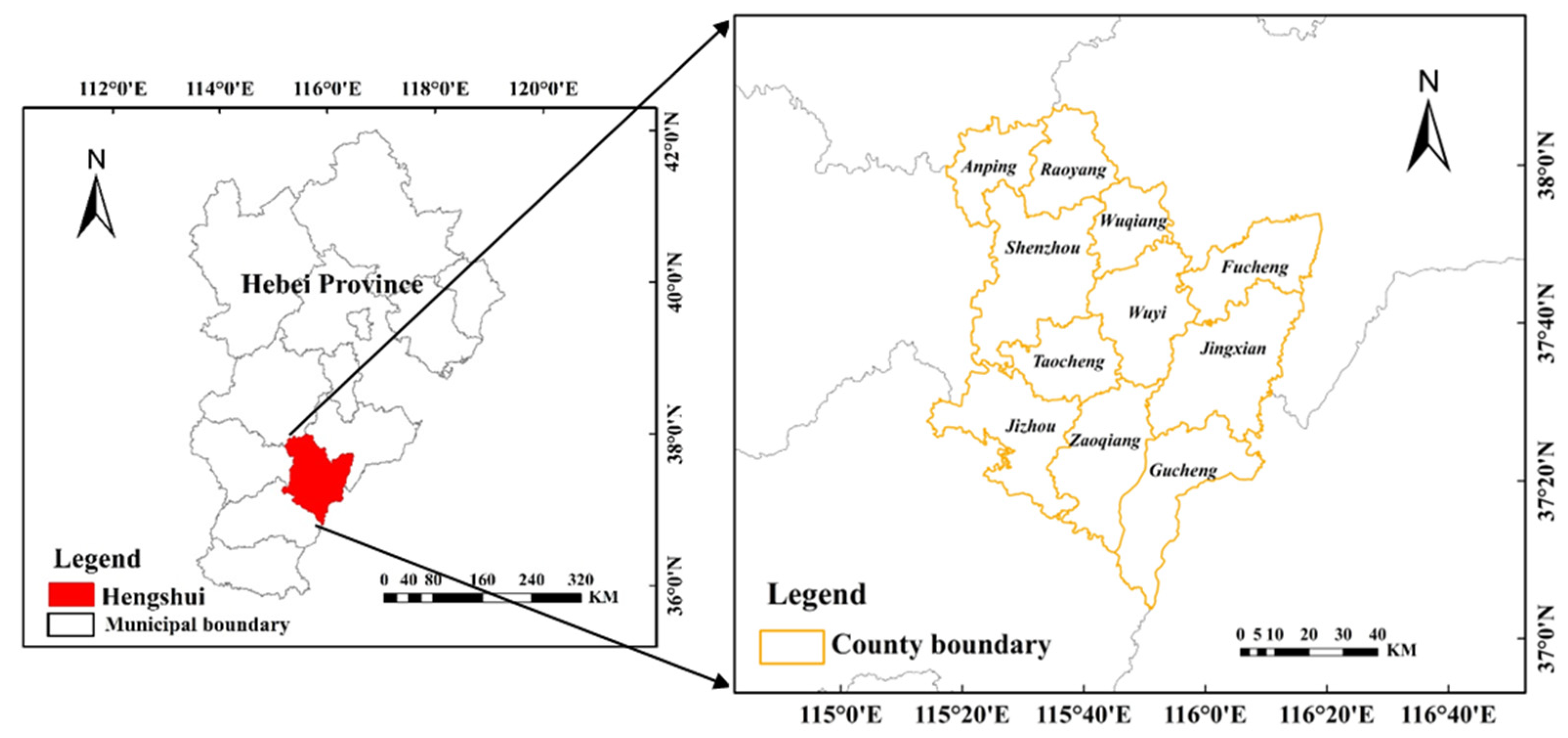
2.1. Study Area

The study area is located in Hengshui, Hebei Province, China, between 115°10′–116°34′ E longitude and 37°03′–38°23′ N latitude, covering two municipal districts, one county-level city, and eight counties, as of 2016 (Figure 1). According to the second soil census, the city’s tidal soil subclass covers 430,000 hectares, accounting for 62% of the total land area, which is widely distributed in all counties and urban areas and is the main soil type for agricultural land. The annual precipitation in Hengshui is 5.66 billion cubic metres, with an average precipitation of 642.1 mm. It belongs to the continental monsoon climate zone, which is warm and semi-arid, and the main types of crops it grows are wheat, corn, sorghum, etc. By 2021, the sown area of grain in Hengshui reached 7191.33 km², of which 3333.3 km² is occupied by winter wheat, accounting for about 1/2 of the sown area of grain in Hengshui. With a total yield of 4.34 billion kg, so the yield of winter wheat has a key influence on the economic development of Hengshui. This study was conducted on winter wheat, which is generally sown in early October and matures in mid-to-late June of the following year in Hengshui. The phenological period of winter wheat is mainly divided into six stages, sowing (early October), tillering (late-November to mid-December), reviving stage (late-February–mid-March), jointing (mid-March–mid-April), tasseling (late-April–mid-May), and mature milking (late-May–mid-June) [32,33].

2.2. Winter Wheat Yield and Planting Distribution

The historical county-level winter wheat yield data record of Hengshui City came from the 2005–2019 statistical yearbook sharing platform, recording yield data (unit: kg/ha). In Hengshui City, there are two municipal districts and one county-level city; there are 11 counties, since we all consider these to be county-level levels. Spatial distribution data of winter wheat in Hengshui at 250 m spatial resolution from 2005–2019 were provided by Chinese Academy of Agricultural Sciences [34]. The extraction results were evaluated in terms of area quantity and spatial location, and the average relative error of area quantity compared with the statistical yearbook for 20 years was 16.1%. In terms of spatial location, the extraction results of 2015 were verified by selecting sample points in Google Earth high-resolution historical images, and the overall accuracy was 86.8% with a kappa coefficient of 0.69. The results indicated that the winter wheat distribution data had a high extraction accuracy.

2.3. Remote Sensing Data

The NASA Terra MODIS vegetation index (VI) products (MOD13Q1, Version 6.1) provide consistent spatial and temporal time series comparisons of global vegetation conditions that can be used to monitor the Earth’s terrestrial photosynthetic vegetation activity in support of phenologic, change detection, and biophysical interpretations. In this study, NDVI and EVI data from the NASA-produced MOD13Q1 dataset with a temporal resolution of 16 days and a spatial resolution of 250 m were used. The MOD15A2H product provides a terrestrial LAI at 500 m resolution every 8 days, and it has been available since 2000 and allows analysis of LAI time series data over multiple growing seasons over long periods of time.

2.4. Gross Primary Productivity

Gross primary productivity (GPP) is the amount of organic carbon fixed by photosynthesis per unit time by organisms, mainly green plants. MOD17A2H offers GPP products as 8-day, 500 m resolution composite products. This data product uses MODIS land cover data, leaf area index, photosynthetically active radiation fraction, and meteorological data from DAO and is fed into a light energy utilisation model. It is important for crop yield estimation, global carbon, and carbon trade [35,36].

2.5. Meteorological Data

In this study, we collected from TerraClimate datasets a dataset of high spatial resolution (1/24°, ~4 km) monthly climate and climatic water balance for global terrestrial surfaces from 1958–2015 [37]. TerraClimate uses climate-assisted interpolation to combine high spatial resolution climate normals from the WorldClim dataset with coarser resolution time-varying (i.e., monthly) data from other sources to generate monthly datasets of precipitation, maximum and minimum temperatures, wind speed, vapour pressure, and solar radiation. This dataset has been widely used by many scholars to calculate various drought indices to assess the effects of drought on vegetation physiological activity and yield [38,39,40,41]. The main climate variables chosen for this paper include precipitation (pr), maximum temperature (tmmx), downgradient surface shortwave radiation (srad), and the Palmer drought index (Pdsi).

2.6. Data Preprocessing

Based on the spatial resolution of winter wheat planting area in Hengshui City being 250 m, in order to maintain the consistent spatiotemporal resolution of all data, we resampled satellite vegetation index, GPP, and meteorological data to 250 m and one-month intervals. Satellite and meteorological data were masked using the distribution of winter wheat cultivation from 2005 to 2019, and all variables of the county-wide monthly average were summarized. All data are pre-processed on the Google Earth Engine (GEE) platform, a free geoprocessing service launched by Google, which provides a large number of geoprocessing algorithms and massive image datasets based on the Google Cloud Platform, and the summary of data is performed on Python and Excel.

3. Methodology

3.1. Long Short-Term Memory

The LSTM network was proposed by Hochreiter et al. [42] in 1997 based on an extension of RNN, which is mainly used to solve the problems that exist in traditional RNN, both gradient disappearance and explosion. The most fundamental difference between RNN and LSTM is that the hidden layer of the LSTM network is a gated unit, where information is added and removed through a ‘gate’ structure that learns which information to keep or forget during training. The LSTM has three types of gate structures: forgetting gates, input gates, and output gates (Figure 2a).

The forgetting gate will decide which information should be forgotten from the neural network unit states, which is implemented by a sigmoid function. The gate is determined by the previous output, H_t−1, and the new input, X_t, to determine which information was removed from the previous cell state, C_t−1. The output is a number between 0 and 1, where 0 means that the information is completely discarded, and 1 means that the information is completely retained, and is calculated as in Equation (1):

$$f_t=\sigma \left(W_f.\left[X_t,H_{t-1}\right]+b_f\right)$$

(1)

where σ is the sigmoid function, f_t is the forgetting gate, H_t−1 denotes the output of the previous node, X_t denotes the current input, W_f is the forgetting gate weight, and b_f is the forgetting gate bias.

The input gate determines which information should be stored from the neural network unit states. Implementing this requires two steps: first the sigmoid layer generates the activation value, i_t, for the input gate based on H_t−1 and X_t. The tanh function creates a candidate vector state, c_t′, which is the alternative to be used for the update, calculated as in (2) and (3):

$$i_t=\sigma \left(W_i.\left[X_t,H_{t-1}\right]+b_i\right)$$

(2)

$$c_t^{\prime }=tanh\left(W_C.\left[X_t,H_{t-1}\right]+b_c\right)$$

(3)

where i_t denotes the input gate output, c_t′ denotes the current candidate node state, W_i and W_c denote the weights of the input gate and the input candidate unit, respectively, and b_i and b_c denote the bias of the input gate and the input candidate unit, respectively. The old cell state, C_t−1, is updated to the new cell state, C_t, using the results obtained from the first two orders, calculated as in (4):

$$C_t=f_t.C_{t-1}+i_t. c_t^{\prime }$$

(4)

Finally there is the output gate, which determines which information in the cell state will be taken as the output of the current state. The sigmoid layer is first run, which determines which cell states are output; then the tanh value of the cell state is multiplied by the output of the sigmoid (normalize the output value) threshold, which ultimately gives the output new cell state H_t, calculated as in (5) and (6).

$$O_t=\sigma \left(W_o.\left[X_t,H_{t-1}\right]+b_o\right)$$

(5)

$$H_t=O_t.\tan \mathrm{h}\left(C_t\right)$$

(6)

where O_t denotes the output gate output, H_t−1 denotes the output of the previous node, X_t denotes the current input, W_o denotes the output gate weight, and b_o denotes the output gate bias.

In this study, the deep neural network model of LSTM winter wheat yield estimation based on the phenological stages is shown in Figure 2b. The input layers of this model are VIs, LAI, GPP, pr, tmmx, srad, and Pdsi for six growing stages of winter wheat. Two layers of LSTM layers are set, and other hyperparameters are set according to the results of Bayesian optimization algorithm in Section 3, with a total of six times steps. To prevent overfitting of the training data a dropout layer is added to the network architecture. All input data need to be normalized before being fed into the model and, finally, back-normalised for output. The ratio of training data to test data is set to 8:2, where 80% is training data and 20% is test data.

3.2. Bayesian Optimization of LSTM Hyperparameters

The process of building LSTM network models involves the determination of many hyperparameters, such as network depth, learning rate, batch size, and so on. The most intuitive way is to find the optimal parameters by manual trial and error, but the manual trial and error method is too inefficient. It lacks a certain exploration process, and the parameters can only be adjusted manually repeatedly for different problems and data. It takes a lot of time, and the final combination of model hyperparameters may not be optimal, which will affect the prediction of the model, including the degree of network fit and the generalization ability to the test set [43,44]. Bayesian optimization, as a very effective global optimization algorithm, requires only a small number of iterations to obtain a desired solution by designing a proper probabilistic agent model and a payoff function [43,44]. The main optimized hyperparameters and the range of values are shown in

Table 1. LSTM hyperparameter setting and range.

Parameters	Range	Parameter Meaning
NumHiddenUnits	(200, 600)	Number of hidden units
MaxEpochs	(200, 800)	Maximum number of epochs
MiniBatchSize	(8, 20)	Size of mini batch
InitialLearnRate	0.01	Initial learning rate
Dropout	(0.1, 0.7)	Abstention factor
SolverName	adam	Solver for training network
LearnRateSchedule	piecewise	Learning rate strategy
Objective function	RMSE

.

The number of hidden units corresponds to the amount of information remembered between time steps (the hidden state). The hidden state can contain information from all previous time steps, regardless of the sequence length. If the number of hidden units is too large, then the layer might overfit to the training data.

Epoch indicates the number of iterations of the data set during model training. If the number of iterations is set too large, the training time of the model is longer, resulting in overfitting of the model, over-reliance on training data, and poor prediction of unknown data, which makes the generalization ability of the model lower. If the number of iterations is set too small, it will make the model fit poorly and affect the prediction accuracy of the model.

Size of the mini-batch to use for each training iteration is indicated, specified as the comma-separated pair consisting of ‘MiniBatchSize’ and a positive integer. A mini-batch is a subset of the training set that is used to evaluate the gradient of the loss function and update the weights. If the number of iterations is set too large, the training time of the model is long, causing the model to be overfitted and overly dependent on the training data. The prediction ability of the unknown data is poor, thus making the generalization ability of the model lower. If the number of iterations is set too small, it will make the model not fit well and affect the prediction accuracy of the model.

The initial learning rate, α, is a relatively important hyperparameter in the LSTM model. When the learning rate is too large, it will cause the parameters to be optimized to fluctuate around the minimum value, thus skipping the optimal solution. When the learning rate is set too small, it will affect the convergence speed of the model, resulting in a slow convergence rate. In this paper, α is set to 0.01 based on the empirical value.

Dropout means that, during the training process of the model, for the network units, they are temporarily dropped from the network according to a certain probability. This hyperparameter plays a crucial role in preventing model overfitting and improving the generalization ability of the model.

The key hyperparameters searched in this paper are data batch size, number of iterations, discard factor, and number of nodes in the hidden layer. The remaining hyperparameters are based on experience, the optimizer is selected as “adam”, LearnRateSchedule is set to “piecewise”, and the root mean square error is selected as the target loss function.

The optimization of the LSTM network model hyperparameters using the Bayesian method is a five-step process as follows (Figure 3, the implementation of the whole process is implemented in matlab R2021b):

Step 1: All data of six winter wheat phenological periods are normalized to divide the training set and validation set for parameter learning and model result validation of the training network model.

Step 2: The LSTM hyperparameters to be optimized and the range are set; a random set of initialized hyperparameters as the initial hyperparameters of the LSTM model are generated. The training set is input for the training of the LSTM neural network. The RMSE is used as the objective function for the hyperparameter optimization of the LSTM model.

Step 3: Gaussian process is used to find the posterior probability distribution of the objective function. The hyperparameter sample points are selected in the modified Gaussian model according to the acquisition function. The acquisition function chosen in this paper is ‘expected-improvement-plus’, which gives preference to the optimal hyperparameter to achieve the update of the hyperparameter.

Step 4: The number of iterations (40) is completed and the minimum objective function and the corresponding trained LSTM model hyperparameters are returned.

Step 5: The validation set is fed into the trained LSTM model to construct an LSTM winter wheat yield estimation model based on Bayesian optimization algorithm.

The general framework of this study is shown in Figure 3a. Based on the indicators required for winter wheat phenology calculation, the influence of different input variables on winter wheat yield prediction was analysed on the BO-LSTM model. Then the performance of different prediction models for winter wheat yield estimation was compared; finally, the robustness of BO-LSTM was explored. All models used were run in matlab R2021b environment.

Figure 3. (a) A research framework of BO-LSTM neural network model for county-level winter wheat yield estimation; (b) Bayesian optimization of LSTM hyperparameters process.

Figure 3. (a) A research framework of BO-LSTM neural network model for county-level winter wheat yield estimation; (b) Bayesian optimization of LSTM hyperparameters process.

3.3. Model Performance Evaluation

In this study, coefficient of determination (R²), root mean square error (RMSE), and mean absolute percentage error (MAPE) were used as indicators to assess the model performance [45]. The equations are written as follows:

$$R^2={\left[\frac{{\displaystyle \sum }(o_i-\overline{o})(y_{i-}\overline{y})}{\sqrt{{\displaystyle \sum }{(o_i-\overline{o})}^2{(y_{i-}\overline{y})}^2}}\right]}^2$$

(7)

$$RMSE=\sqrt{\frac{1}{n}{\displaystyle \sum }_{i=1}^n{(o_{i-}{y}_i)}^2}$$

(8)

$$MAPE=\frac{1}{n}{\displaystyle \sum }_{i=1}^n\left|\frac{y_i-o_i}{y_i}\right|$$

(9)

where n is the number of samples, and y_i and o_i are the measured and predicted values of winter wheat yield, respectively. R² is a measure of the strength of the linear relationship between the predicted and measured values of the model, with larger R² indicating that the measured and predicted values have similar trends. RMSE is used to assess the deviation between measured and predicted values. The smaller the value, the smaller the deviation is between the measured and predicted values of the model; the higher R², the smaller RMSE is and the better the model. For the MAPE range [0, +∞), the smaller the MAPE, the better the model simulation results are. Compared to RMSE, MAPE is equivalent to normalizing the error at each point, reducing the effect of absolute error from individual outliers.

4. Results and Analysis

4.1. Performance of LSTM Hyperparameter Combination Output Based on Bayesian Optimization

This study aims to optimise the hyperparameters of the LSTM neural network model based on a Bayesian optimisation algorithm, evaluating both the time efficiency, “time”, and the accuracy, RMSE, of the model after tuning the parameters. The first three optimal parameter combinations were selected, along with the corresponding accuracy and time consumption (

Table 2. Output results of Bayesian optimized LSTM hyperparameters on the training set.

Methods	NumOfUnits	MaxEpochs	MinBatchSize	DropoutLayer	Time/min	RMSE
Bayesian optimization	202	314	9	0.1	14	149.51
	335	501	10	0.1	14	181.57
	354	510	11	0.025	14	182.80

). The results demonstrate that the minimum RMSE of the Bayesian optimised LSTM model on the training set is 149.51 kg/ha, and the time efficiency of finding the optimal hyperparameter combination is 14 min. The Bayesian optimisation algorithm makes full use of historical information when selecting the optimal hyperparameter combination, allowing the optimal hyperparameter combination to be found within a short time and number of iterations.

4.2. Yield Estimation Performance for Different Combinations of Inputs

To evaluate the performance of yield estimation from different data sources, we put different combinations of input variables in a BO-LSTM model for analysis. Figure 4 shows the yield estimation performance of BO-LSTM for winter wheat with five different input variables. We found that yield estimates using GPP (R² = 0.72, RMSE = 186.13 kg/ha) alone were more accurate than those using LAI (R² = 0.67, RMSE = 221.32 kg/ha) alone. When combined with meteorological data, the accuracy of GPP combined with meteorological data was higher (R² = 0.81, RMSE = 180.66 kg/ha) compared to the remotely sensed vegetation index (R² = 0.78, RMSE = 190.96 kg/ha), because GPP more directly reflects the process of organic matter accumulation by vegetation photosynthesis. The yield estimation accuracy of winter wheat gradually increased as the input data increased, indicating that the estimation accuracy of fusing multiple sources of data was better than the input from a single data source. The highest estimation accuracy was achieved by integrating all data together (R² = 0.83, RMSE = 177.84 kg/ha). The addition of the data improved the model’s ability to capture spatial heterogeneity in yield, capturing more features associated with winter wheat yield. In particular, the yield estimation accuracy of the LSTM model improved significantly when combined with meteorological data, suggesting that meteorological data provide unique and irreplaceable information.

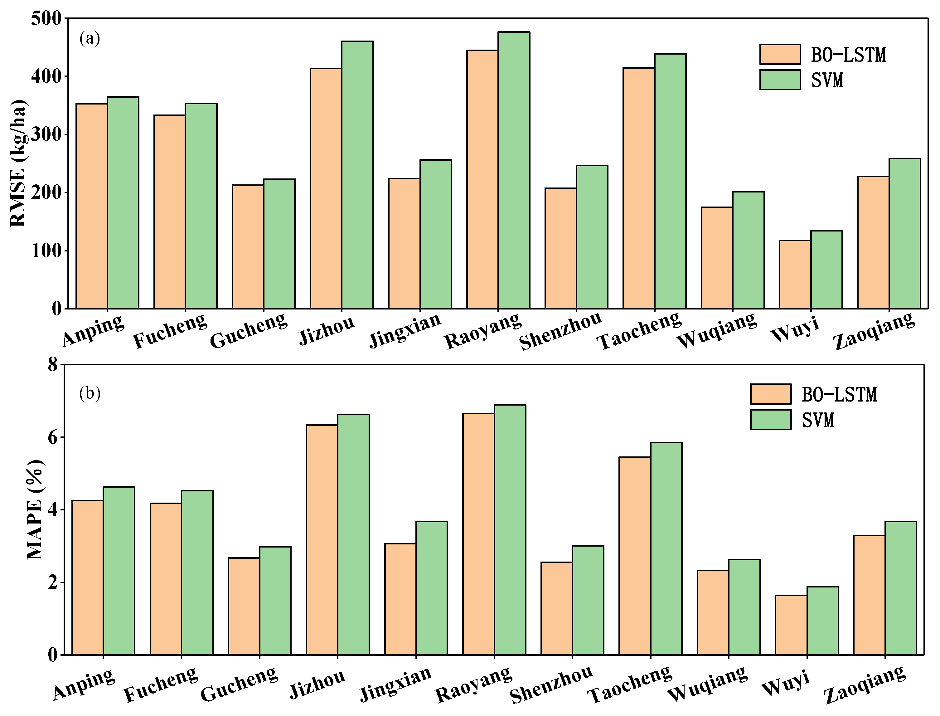
4.3. Comparison with Other Methods

The analysis in the previous section led us to conclude that the highest accuracy in winter wheat yield estimation can be achieved by integrating all data, so we used data with “GPP + Climate + LAI + VIs” as the final input data for the BO-LSTM. To further evaluate the yield estimation performance of the BO-LSTM, we used a machine learning SVM and a linear regression Lasso to estimate the yield of winter wheat. Figure 5 presents a scatter plot of our yield estimates and statistical annals for all county test data for Hengshui city using the three prediction models. Based on the R² and RMSE values, it can be intuitively seen that the SVM (RMSE = 185.7 kg/ha, R² = 0.80) and BO-LSTM (RMSE = 177.8 4 kg/ha, R² = 0.82) model methods perform significantly better than Lasso (RMSE = 214.5 kg/ha, R² = 0.76). The potential reason could be that SVM and BO-LSTM methods capture the complex and nonlinear relationships between input variables and winter wheat yield better than linear regression models. Further, it is found that the BO-LSTM model slightly outperformed the SVM method in estimating winter wheat yield in Hengshui City. This is largely attributed to the fact that machine learning non-temporal models focus on information extraction for unordered data and do not optimize the structure for temporal data. The LSTM is a recurrent neural network structure that transmits cumulative effective information during different growth stages. It is similar to the growth process characteristics of crops: crop growth and progressive developmental changes and biomass accumulation. The effects of environmental factors on winter wheat yield are complex and non-linear. The LSTM inputs the observations into the model network structure in a temporal order, and the gate mechanism is set internally. The weights of input gates, forgetting gates, and input gates are trained to achieve automatic screening and fusion of timing features.

Immediately afterwards, we used the BO-LSTM with better estimation accuracy and SVM to estimate winter wheat yield for all counties in Hengshui (Figure 6). In general, there was some spatial variation in the estimation advantage of different regions. The estimation performance of BO-LSTM was still slightly higher than that of SVM, regardless of the county region. Using the BO-LSTM model with better yield estimation accuracy, we can see that the RMSE is more than 300 kg/ha in RaoYang County, Jizhou City, Taocheng District, Anping County, and Fucheng County. The highest is in Rao Yang County with an RMSE of 444. 77 kg/ha and a MAPE of 6.18. The areas with RMSE between 200–300 kg/ha are Shecheng County, Jing County, Shenzhou City, and Zaojiang County. Areas with RMSE less than 200 kg/ha include Wuyi County and Wuqiang County, with the smallest being located in Wuyi County (RMSE = 117.30 kg/ha, MAPE = 1.64).

5. Discussion

In this study we highlight the advantages of BO-LSTM fusing multi-source data for winter wheat yield estimation. The results show that the deep learning model fusing multi-source data provides reliable winter wheat yield estimation at the regional scale. In general, GPP, LAI, and VIs are suitable for large-scale crop yield estimation. The estimation accuracy can be improved by combining meteorological data. The highest estimation accuracy is achieved when all predictors are combined and entered into the estimation model, which is very similar to previous studies [25,46,47]. Since this paper uses SVM, LSTM, and LASSO as the yield estimation models, which are regularized, we do not need to consider the problem of multicollinearity.

The Bayesian optimizer can determine an acceptable value very quickly, which is especially advantageous when the time complexity of finding the value of any function of the black box function is high, and the Bayesian optimizer does not have a limit on the search fineness. The disadvantage is that the returned result is not necessarily the true minimum objective function value (grid search may not find it either), and the result of each optimization will vary. Therefore, several optimizations are needed when optimizing the LSTM hyperparameters with Bayesian, and the best optimization result is finally selected.

For the problem of different estimation accuracies in different regions (Figure 6), we analysed the distribution of winter wheat cultivation over 15 years and found that we only listed four of them (Figure 7), and the distribution of wheat cultivation in Taocheng, Jizhou, Anping, and Rao Yang regions was more scattered with less cultivated area. Among them, Taocheng District and Jizhou District are the city centre of Hengshui City. The marginal effects of various factors in cities within a certain region affect climate factors, and local climate is difficult to obtain accurately compared to other regions, resulting in differences between the meteorological data we obtained and the actual meteorological data [48]. This explains the large discrepancy between estimated yields and official yield records in these areas. Our method is therefore more suitable for areas where the distribution of cultivation is concentrated, far from urban building sites, and with relatively little human interference.

In the process of analysis, we found that there are still some limitations. The first is that we focus on estimating county-level crop yields, which leads to smaller training samples due to the difficulty of obtaining data. The problem of data scarcity makes the learning information aspect of the LSTM neural network model insufficient in the training process. Second, the essence of deep learning is feature extraction from data to data, and neural network modelling converts the original input variables into high-level representations through nonlinear activation and squeeze functions. The description and mechanistic expression of the crop growth process cannot be learned, which weakens the traceability and interpretability of the LSTM model. The data-driven crop growth model has great potential. The crop growth model can take the crop, environment, and cultivation technology as a whole. The principles and methods of systems analysis can be applied to provide theoretical generalizations and quantitative analyses of the physiological processes of crop growth and development, photosynthetic production, organogenesis, and yield formation and their feedback relationships to environment and technology. Following that, the corresponding mathematical models are developed to carry out the dynamic quantitative simulation of the crop growth process. Therefore, fusing deep learning with crop mechanism models can improve the interpretability of deep learning models. To address the problems, our future work focuses on expanding the study area to integrate process-based models and deep learning techniques to develop hybrid models. The BO-LSTM model provides a data-driven approach to crop growth time series feature extraction by combining the crop weathering characteristics. The spatiotemporal scalability of the BO-LSTM model is worth exploring in future research. The spatial transfer learning capability of the BO-LSTM can be evaluated to quantify the model’s ability to estimate crop yields in areas without many historical yield records. A deep learning approach based on BO-LSTM to learn the spatiotemporal heterogeneity of crop growth can help to better understand the impact of global climate change on agricultural production.

6. Conclusions

In this research, we proposed a BO-LSTM model that integrates crop phenology and meteorological and remote sensing data to predict county-level winter wheat yields. Yield estimation performance was then compared using three predictive models, including linear regression, machine learning, and deep learning. The conclusions are as follows:

(1)

Using Bayesian optimization of LSTM neural network model hyperparameters can achieve identification of the optimal combination of hyperparameters in a shorter period of time.

(2)

Multi-temporal remote sensing data based on BO-LSTM model combined with meteorological data can provide effective information to obtain more accurate yield prediction models to estimate regional scale winter wheat yield.

(3)

Among the three prediction models, BO-LSTM achieves higher yield estimation accuracy relative to Lasso and SVM.

(4)

There is some spatial variation in the estimated yield advantage in different areas, and our method is more suitable for places where crop cultivation is concentrated, far from urban building sites and with less residential land.

References

1. Shewry, P.-R.; Hey, S.-J. The contribution of wheat to human diet and health. Food Energy Secur. 2015, 4, 178–202. [Google Scholar] [CrossRef]
2. Tilman, D.; Balzer, C.; Hill, J.; Befort, B.L. Global food demand and the sustainable intensification of agriculture. Proc. Natl. Acad. Sci. USA 2011, 108, 20260–20264. [Google Scholar] [CrossRef] [Green Version]
3. Lesk, C.; Rowhani, P.; Ramankutty, N. Influence of extreme weather disasters on global crop production. Nature 2016, 529, 84–87. [Google Scholar] [CrossRef] [Green Version]
4. Lesk, C.; Coffel, E.; Winter, J.; Ray, D.; Zscheischler, J.; Seneviratne, S.-I.; Horton, R. Stronger temperature–moisture couplings exacerbate the impact of climate warming on global crop yields. Nat. Food 2021, 2, 683–691. [Google Scholar] [CrossRef]
5. Chipanshi, A.; Zhang, Y.; Kouadio, L.; Newlands, N.; Davidson, A.; Hill, H.; Warren, R.; Qian, B.; Daneshfar, B.; Bedard, F.; et al. Evaluation of the Integrated Canadian Crop Yield Forecaster (ICCYF) model for in-season prediction of crop yield across the Canadian agricultural landscape. Agric. For. Meteorol. 2015, 206, 137–150. [Google Scholar] [CrossRef] [Green Version]
6. Yan, K.; Pu, J.; Park, T.; Xu, B.; Zeng, Y.; Yan, G.; Weiss, M.; Knyazikhin, Y.; Myneni, R.-B. Performance stability of the MODIS and VIIRS LAI algorithms inferred from analysis of long time series of products. Remote Sens. Environ. 2021, 260, 112438. [Google Scholar] [CrossRef]
7. de la Casa, A.; Ovando, G.; Díaz, G. Linking data of ENSO, NDVI-MODIS and crops yield as a base of an early warning system for agriculture in Córdoba, Argentina. Remote Sens. Appl. 2021, 22, 100480. [Google Scholar]
8. Son, N.T.; Chen, C.F.; Chen, C.R.; Chang, L.Y.; Duc, H.N.; Nguyen, L.D. Prediction of rice crop yield using MODIS EVI−LAI data in the Mekong Delta, Vietnam. Int. J. Remote Sens. 2013, 34, 7275–7292. [Google Scholar] [CrossRef]
9. Peng, B.; Guan, K.; Zhou, W.; Jiang, C.; Frankenberg, C.; Sun, Y.; He, L.; Köhler, P. Assessing the benefit of satellite-based Solar-Induced Chlorophyll Fluorescence in crop yield prediction. Int. J. Appl. Earth Obs. Geoinf. 2020, 90, 102126. [Google Scholar] [CrossRef]
10. Sakamoto, T.; Gitelson, A.A.; Arkebauer, T. MODIS-based corn grain yield estimation model incorporating crop phenology information. Remote Sens. Environ. 2013, 131, 215–231. [Google Scholar] [CrossRef]
11. Hao, S.; Ryu, D.; Western, A.; Perry, E.; Bogena, H.; Franssen, H.J.H. Performance of a wheat yield prediction model and factors influencing the performance: A review and meta-analysis. Agric. Syst. 2021, 194, 103278. [Google Scholar] [CrossRef]
12. Jones, E.J.; Bishop, T.F.A.; Malone, B.P.; Hulme, P.J.; Whelan, B.M.; Filippi, P. Identifying causes of crop yield variability with interpretive machine learning. Comput. Electron. Agric. 2022, 192, 106632. [Google Scholar] [CrossRef]
13. Wang, M.M.; Rengasamy, P.; Wang, Z.C.; Yang, F.; Ma, H.Y.; Huang, L.H.; Liu, M.; Yang, H.Y.; Li, J.P.; An, F.H.; et al. Identification of the most limiting factor for rice yield using soil data collected before planting and during the reproductive stage. Land Degrad. Dev. 2018, 29, 2310–2320. [Google Scholar] [CrossRef]
14. Hernández, C.M.; Faye, A.; Ly, M.O.; Stewart, Z.P.; Vara Prasad, P.V.; Bastos, L.M.; Nieto, L.; Carcedo, A.J.P.; Ciampitti, I.A. Soil and Climate Characterization to Define Environments for Summer Crops in Senegal. Sustainability 2021, 13, 11739. [Google Scholar] [CrossRef]
15. Chu, Z.; Yu, J. An end-to-end model for rice yield prediction using deep learning fusion. Comput. Electron. Agric. 2020, 174, 105471. [Google Scholar] [CrossRef]
16. Tedesco-Oliveira, D.; Pereira Da Silva, R.; Maldonado, W.; Zerbato, C. Convolutional neural networks in predicting cotton yield from images of commercial fields. Comput. Electron. Agric. 2020, 171, 105307. [Google Scholar] [CrossRef]
17. Maimaitijiang, M.; Sagan, V.; Sidike, P.; Hartling, S.; Esposito, F.; Fritschi, F.B. Soybean yield prediction from UAV using multimodal data fusion and deep learning. Remote Sens. Environ. 2020, 237, 111599. [Google Scholar] [CrossRef]
18. Sun, J.; Di, L.; Sun, Z.; Shen, Y.; Lai, Z. County-Level Soybean Yield Prediction Using Deep CNN-LSTM Model. Sensors 2019, 19, 4363. [Google Scholar] [CrossRef] [Green Version]
19. Nevavuori, P.; Narra, N.; Lipping, T. Crop yield prediction with deep convolutional neural networks. Comput. Electron. Agric. 2019, 163, 104859. [Google Scholar] [CrossRef]
20. Rumelhart, D.-E.; Hinton, G.-E.; Williams, R.-J. Learning representations by back-propagating errors. Nature 1986, 323, 533–536. [Google Scholar] [CrossRef]
21. Zhang, L.; Zhang, Z.; Luo, Y.; Cao, J.; Tao, F. Combining Optical, Fluorescence, Thermal Satellite, and Environmental Data to Predict County-Level Maize Yield in China Using Machine Learning Approaches. Remote Sens. 2019, 12, 21. [Google Scholar] [CrossRef]
22. Greff, K.; Srivastava, R.K.; Koutnik, J.; Steunebrink, B.R.; Schmidhuber, J. LSTM: A Search Space Odyssey. IEEE Trans. Neural Netw. Learn. Syst. 2017, 28, 2222–2232. [Google Scholar] [CrossRef] [Green Version]
23. Haider, S.; Naqvi, S.; Akram, T.; Umar, G.; Shahzad, A.; Sial, M.; Khaliq, S.; Kamran, M. LSTM Neural Network Based Forecasting Model for Wheat Production in Pakistan. Agronomy 2019, 9, 72. [Google Scholar] [CrossRef] [Green Version]
24. Jiang, H.; Hu, H.; Zhong, R.; Xu, J.; Xu, J.; Huang, J.; Wang, S.; Ying, Y.; Lin, T. A deep learning approach to conflating heterogeneous geospatial data for corn yield estimation: A case study of the US Corn Belt at the county level. Glob. Chang. Biol. 2020, 26, 1754–1766. [Google Scholar] [CrossRef]
25. Tian, H.; Wang, P.; Tansey, K.; Zhang, J.; Zhang, S.; Li, H. An LSTM neural network for improving wheat yield estimates by integrating remote sensing data and meteorological data in the Guanzhong Plain, PR China. Agric. For. Meteorol. 2021, 310, 108629. [Google Scholar] [CrossRef]
26. Li, L.; Wang, B.; Feng, P.; Wang, H.; He, Q.; Wang, Y.; Liu, D.L.; Li, Y.; He, J.; Feng, H.; et al. Crop yield forecasting and associated optimum lead time analysis based on multi-source environmental data across China. Agric. For. Meteorol. 2021, 308–309, 108558. [Google Scholar] [CrossRef]
27. Batten, A.J.; Thorpe, J.; Piegari, R.I.; Rosland, A. A Resampling Based Grid Search Method to Improve Reliability and Robustness of Mixture-Item Response Theory Models of Multimorbid High-Risk Patients. IEEE J. Biomed. Health Inform. 2020, 24, 1780–1787. [Google Scholar] [CrossRef]
28. Zhang, Y.; Wang, S.; Ji, G.; Wang, S. A Comprehensive Survey on Particle Swarm Optimization Algorithm and Its Applications. Math. Probl. Eng. 2015, 2015, 931256. [Google Scholar] [CrossRef] [Green Version]
29. Mohammed, K.-K.; Hassanien, A.-E.; Afify, H.-M. Classification of Ear Imagery Database using Bayesian Optimization based on CNN-LSTM Architecture. J. Digit. Imaging 2022, 35, 947–961. [Google Scholar] [CrossRef]
30. Goay, C.-H.; Ahmad, N.-S.; Goh, P. Transient Simulations of High-Speed Channels Using CNN-LSTM With an Adaptive Successive Halving Algorithm for Automated Hyperparameter Optimizations. IEEE Access 2021, 9, 127644–127663. [Google Scholar] [CrossRef]
31. Liu, X.; Shi, Q.; Liu, Z.; Yuan, J. Using LSTM Neural Network Based on Improved PSO and Attention Mechanism for Predicting the Effluent COD in a Wastewater Treatment Plant. IEEE Access 2021, 9, 146082–146096. [Google Scholar] [CrossRef]
32. Chen, X.; Wang, W.; Chen, J.; Zhu, X.; Shen, M.; Gan, L.; Cao, X. Does any phenological event defined by remote sensing deserve particular attention? An examination of spring phenology of winter wheat in Northern China. Ecol. Indic. 2020, 116, 106456. [Google Scholar] [CrossRef]
33. Xiao, D.; Tao, F.; Liu, Y.; Shi, W.; Wang, M.; Liu, F.; Zhang, S.; Zhu, Z. Observed changes in winter wheat phenology in the North China Plain for 1981–2009. Int. J. Biometeorol. 2013, 57, 275–285. [Google Scholar] [CrossRef] [PubMed]
34. Du, Y. The Influence of Atmospheric Aerosol’s Direct Radiation Effect on Winter Wheat GPP in North China. Master’s Thesis, Chinese Academy of Agricultural Sciences, Beijing, China, 2021. [Google Scholar]
35. Fu, S.; Kong, L.; Zhou, H.; Liu, W. Spatial|temporal distribution characteristics of grain yield and its potential productivity in the Jing river basin and their relationships with MODIS-GPP. Agric. Res. Arid Areas 2020, 38, 192–199. [Google Scholar]
36. Varghese, R.; Behera, M.-D. Annual and seasonal variations in gross primary productivity across the agro-climatic regions in India. Environ. Monit. Assess. 2019, 191, 631. [Google Scholar] [CrossRef]
37. Abatzoglou, J.T.; Dobrowski, S.Z.; Parks, S.A.; Hegewisch, K.C. TerraClimate, a high-resolution global dataset of monthly climate and climatic water balance from 1958–2015. Sci. Data 2018, 5, 170191. [Google Scholar] [CrossRef] [Green Version]
38. Abdi, O. Climate-Triggered Insect Defoliators and Forest Fires Using Multitemporal Landsat and TerraClimate Data in NE Iran: An Application of GEOBIA TreeNet and Panel Data Analysis. Sensors 2019, 19, 3965. [Google Scholar] [CrossRef] [Green Version]
39. Salvacion, A.-R. Mapping meteorological drought hazard in the Philippines using SPI and SPEI. Spat. Inf. Res. 2021, 29, 949–960. [Google Scholar] [CrossRef]
40. Gómez-Pineda, E.; Hammond, W.M.; Trejo-Ramirez, O.; Gil-Fernández, M.; Allen, C.D.; Blanco-García, A.; Sáenz-Romero, C. Drought years promote bark beetle outbreaks in Mexican forests of Abies religiosa and Pinus pseudostrobus. For. Ecol. Manag. 2022, 505, 119944. [Google Scholar] [CrossRef]
41. Cao, J.; Zhang, Z.; Tao, F.; Zhang, L.; Luo, Y.; Zhang, J.; Han, J.; Xie, J. Integrating Multi-Source Data for Rice Yield Prediction across China using Machine Learning and Deep Learning Approaches. Agric. For. Meteorol. 2021, 297, 108275. [Google Scholar] [CrossRef]
42. Sepp, H.; Jürgen, S. Long short-term memory. Neural Comput. 1997, 9, 1735–1780. [Google Scholar]
43. Huang, W. Study on the Effect of LSTM Hyper-Parameter Tuning for Prediction of River Discharge. J. Xihua Univ. 2020, 39, 23–29. [Google Scholar]
44. Jiang, M.; Chen, Y. Survey on Bayesian optimization algorithm. Comput. Eng. Des. 2010, 31, 3254–3259. [Google Scholar]
45. Lin, L.-I.-K. A Concordance Correlation Coefficient to Evaluate Reproducibility. Biometrics 1989, 45, 255. [Google Scholar] [CrossRef]
46. Feng, P.; Wang, B.; Liu, D.L.; Waters, C.; Xiao, D.; Shi, L.; Yu, Q. Dynamic wheat yield forecasts are improved by a hybrid approach using a biophysical model and machine learning technique. Agric. For. Meteorol. 2020, 285–286, 107922. [Google Scholar] [CrossRef]
47. Liu, Y.; Wang, S.; Wang, X.; Chen, B.; Chen, J.; Wang, J.; Huang, M.; Wang, Z.; Ma, L.; Wang, P.; et al. Exploring the superiority of solar-induced chlorophyll fluorescence data in predicting wheat yield using machine learning and deep learning methods. Comput. Electron. Agric. 2022, 192, 106612. [Google Scholar] [CrossRef]
48. Trindade, F.; Fulginiti, L.-E.; Perrin, R.-K. Crop Yield Growth along the 41st Parallel: Contributions of Environmental vs. Human-Controlled Factors Environmental vs. Human-Controlled Factors. Cornhusker Econ. 2020, 1074. [Google Scholar] [CrossRef]
Figure 1. Location of the study area.
Agronomy 12 03194 g001
Figure 2. (a) The structure of the LSTM neural network; (b) Structure of the phenology-based LSTM model.
Agronomy 12 03194 g002
Figure 4. Winter wheat yield estimation using BO-LSTM for different combinations of data source inputs.
Agronomy 12 03194 g004
Figure 5. Performance of the 2005–2019 test set for winter wheat yield estimation in different forecasting models.
Agronomy 12 03194 g005
Figure 6. BO-LSTM performance of yield estimation for all counties in Hengshui city: (a) RMSE; (b) MAPE.
Agronomy 12 03194 g006
Figure 7. Spatial distribution of winter wheat in Hengshui City, 2016–2019.
Agronomy 12 03194 g007