Rapid and Accurate Prediction of Soil Texture Using an Image-Based Deep Learning Autoencoder Convolutional Neural Network Random Forest (DLAC-CNN-RF) Algorithm

Abstract

Soil determines the degree of water infiltration, crop nutrient absorption, and germination, which in turn affects crop yield and quality. For the efficient planting of agricultural products, the accurate identification of soil texture is necessary. This study proposed a flexible smartphone-based machine vision system using a deep learning autoencoder convolutional neural network random forest (DLAC-CNN-RF) model for soil texture identification. Different image features (color, particle, and texture) were extracted and randomly combined to predict sand, clay, and silt content via RF and DLAC-CNN-RF algorithms. The results show that the proposed DLAC-CNN-RF model has good performance. When the full features were extracted, a very high prediction accuracy for sand (R² = 0.99), clay (R² = 0.98), and silt (R² = 0.98) was realized, which was higher than those frequently obtained by the KNN and VGG16-RF models. The possible mechanism was further discussed. Finally, a graphical user interface was designed and used to accurately predict soil types. This investigation showed that the proposed DLAC-CNN-RF model could be a promising solution to costly and time-consuming laboratory methods.

1. Introduction

In recent decades, new techniques have resulted in significant progress in agriculture. Precision agriculture has become increasingly important in agricultural cultivation and management. Soil is the fundamental productive resource that provides a suitable environment for seed germination and root growth. Soil texture is one of the most important and fundamental parameters to consider when it comes to soil because it greatly influences its physical, chemical, and biological properties [1,2], such as the degree of water and air penetration, nutrient absorption, susceptibility to erosion, and germination. Thus, exact soil texture identification is required for precise agriculture and soil management. A thorough grasp of soil textural heterogeneity can benefit sound agricultural practice in various growing situations.

Conventional mechanical methods used for soil texture analysis entail numerous complex steps, such as drying, crushing, and sieving [3]. Hydrometers and pipettes are extensively used mechanical methods [4]. Although these techniques provide accurate soil textural analysis results, they are time-consuming. Moreover, these methods use H₂O₂ as a corrosive reagent, which is harmful to the environment. The soil textural report can be produced with a large dynamic range and flexibility using an advanced laser diffraction particle size analyzer, but it induces high costs and sampling errors [5,6]. Therefore, new techniques are urgently needed for rapid, cheap, and sophisticated soil texture measurement [7].

Currently, the approaches used for the fast and low-cost measurement of the soil textural parameters rely on extracted texture and color features for further prediction and classification. Recent evidence suggests that the particle size also can be used to identify soil texture using X-ray [8], laser [9], infrared spectroscopy [10], and gamma radiation [11]. For instance, Vohland et al. [12] reported an environmentally friendly method of predicting sand and clay contents using diffuse reflectance infrared Fourier transform spectroscopy (DRIFS) without any chemical agents. Nevertheless, the above-mentioned approaches have not been recognized as standard methods because precise and complicated equipment is required. Furthermore, the particle size distribution should be predetermined before the measurement [13].

With the development of digital technology, cameras and smartphones are gaining popularity in predicting soil parameters, particularly in developing countries with limited budgets. Smartphones have many advantages, including portability, low-cost, and good image acquisition capability. Furthermore, modern digital technology promotes the development of computer vision and deep learning, which are increasingly used for soil image prediction and classification [14]. However, the complex preprocessing steps for preparing soil thin sections remain a problem. A method that combines microscopic image capturing with a continuous wavelet transform (CWT)-based computer vision algorithm has been proposed by Sudarshan et al. [15] to predict soil texture both in situ and ex situ. In those smartphone-based soil image identification studies, soil profile [16], digital RGB photography (combined with neural network modelling) [17], and digital image processing and multivariate image analysis [18] have been explored. Nevertheless, high accuracy is still difficult to realize. There is a lack of comprehensive methods in which soil images can be effectively exploited for soil texture prediction.

As a powerful ensemble learning, random forest (RF) is attracting considerable interest for classification and regression by constructing a multitude of decision trees. Scientists have already proven that RF ensemble exhibits superior prediction than a single tree [19]. For instance, Dornik et al. [20] performed a successful classification of soil types using geographic object-based image analysis. Convolutional neural network (CNN) is also a powerful algorithm widely used in image sensing and object detection [21,22]. A large amount of data from soil images can be successfully processed by CNN. For example, Swetha et al. realized a high prediction accuracy for clay (98%) and sand (98%) and moderate prediction accuracy (75%) for silt using CNN algorithms [23]. Rahim Azadnia et al. [24] predicted soil images at a distance of 20, 40, and 60 cm with an accuracy of 99.89%, 99.81%, and 99.58%, respectively, via a CNN model. However, only 11 soil textures were considered in this work, and the prediction accuracy of the proposed CNN model for the remaining soil texture is unknown.

In this study, a low-cost image acquisition system was constructed, and a method combining the DLAC, CNN, and RF algorithms was established to predict all the soil textures. Image features (color, particle, and texture) with random combinations were extracted. An environmentally friendly graphical user interface has been designed to generate the results. Surprisingly, the proposed DLAC-CNN-RF model obtained a very high average prediction accuracy (99.67% for all the soil textures). This approach provides a promising solution for the accurate identification of soil texture.

2. Materials and Methods

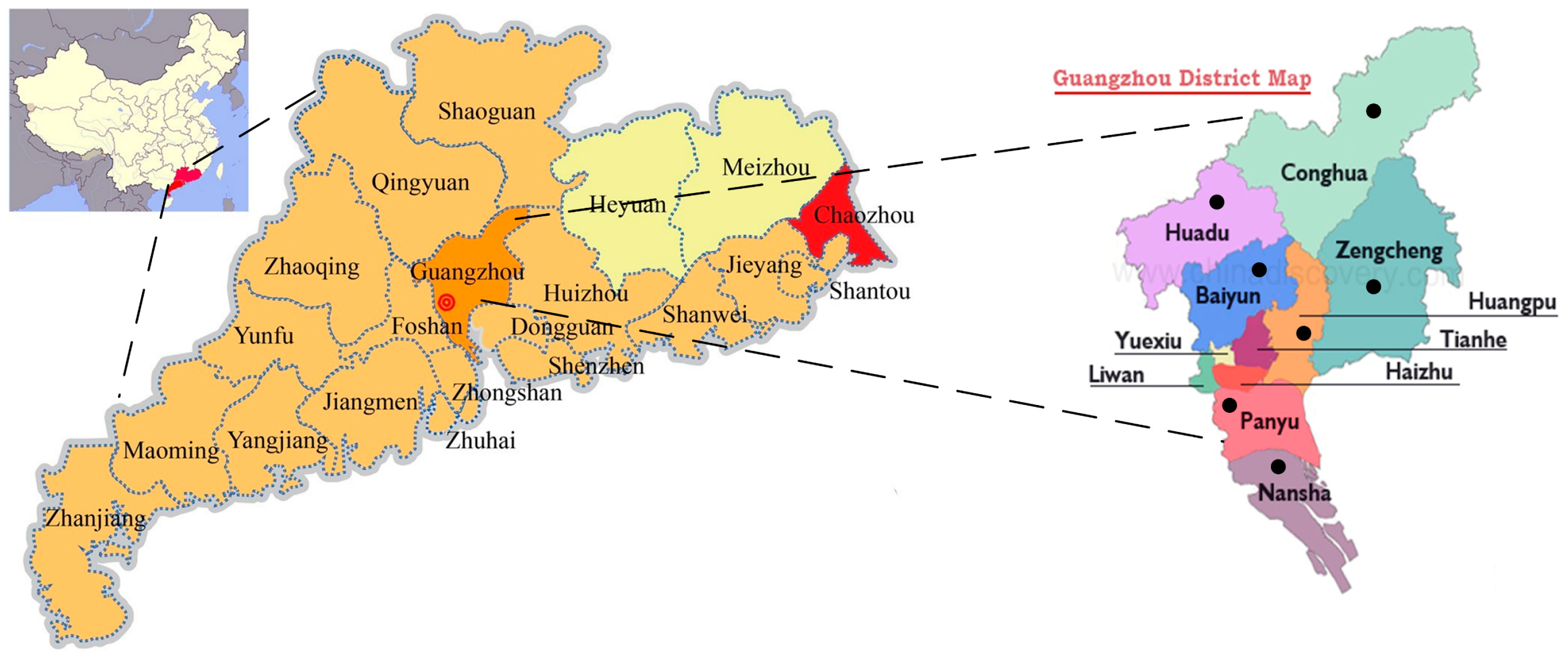
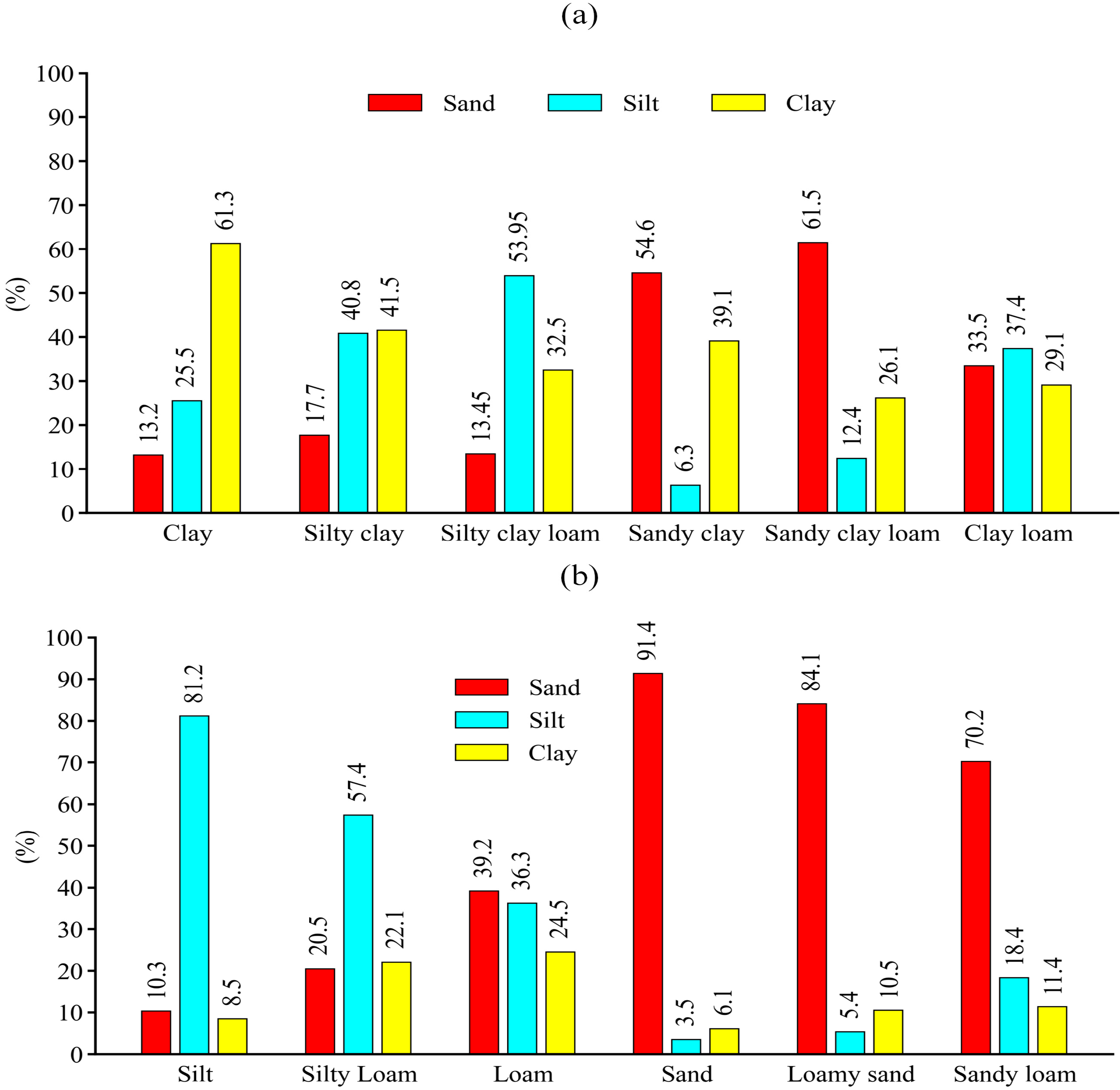
2.1. Sample Preparation

Soil samples were extracted from different areas in Guangzhou City, Guangdong Province (22.26° N~23.56° N, 112°57 E~114.3° E), including the Panyu, Huadu, Conghua, Haizhu, Nansha, Huangpu, and Zengcheng districts (See Figure 1). These regions have the required conditions for growing agricultural products due to their suitable climate and abundant water resources. A total of 1000 samples were taken from the 50 locations distributed in the different city districts. The locations include paddy fields, vegetable gardens, dry land, cane land, and plantain land. Various depths of the soils were collected by a standard shovel, and the depth varied within a range of 0–15 cm from the ground soil surface. To guarantee the purity of the samples, after each sampling, the shovel was cleaned before taking the next sample. The locations of the collected samples were input into a global positioning system receiver (Garmin eTrex 20×) for geolocation analysis. All the samples were collected in a sealed pocket with a label and then shipped back to the Solar Energy Intelligent Irrigation Equipment Technology Innovation Center Laboratory of Guangzhou University for processing.

All the samples were initially air-dried for 24 h with a light intensity of 1.5 × 10⁴ Lux and a wind speed of 16 m/s. Then, the samples were run through a 2 mm sieve to eliminate plant debris and tiny particles. A hydrometer (ASTM mode 152H) method was utilized to measure the average percentage of the sand, silt, and clay particles in each soil texture, mainly because this method gives the benefits of simplicity, reasonable price, and rapid detection. Finally, 12 soil texture types, consisting of clay, silty clay, silty clay loam, sandy clay, sandy clay loam, clay loam, silt, silty loam, loam, sandy, loamy sand, and sand loam, were prepared for imaging.

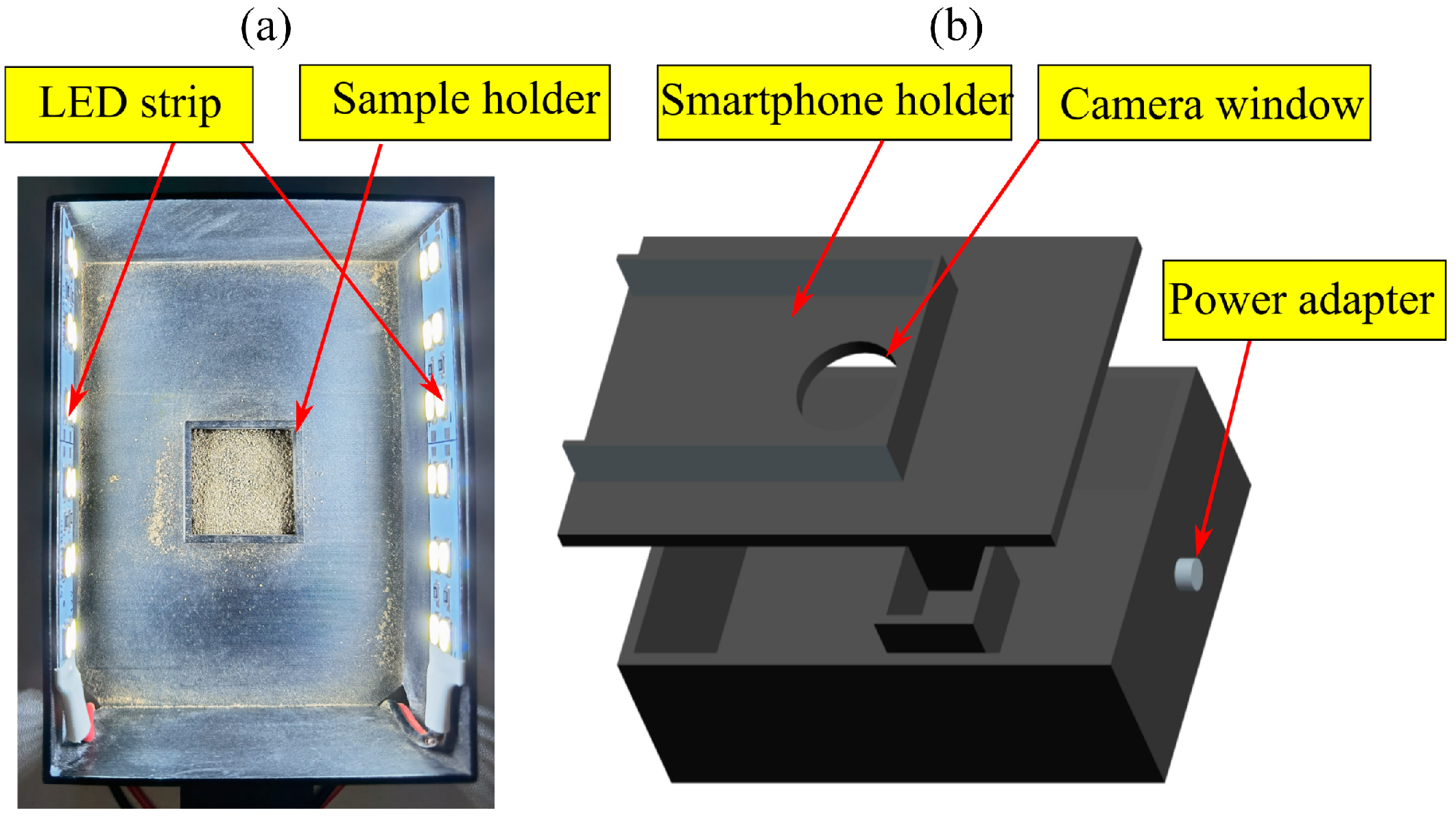
2.2. Image Acquisition

To alleviate ambient light interference, an image acquisition device was designed and fabricated for imaging the soil samples (See Figure 2). A smartphone holder was constructed at the top of the box, and a circular window was opened to hold the camera for taking images. A black chamber (12 cm × 8 cm × 5 cm) was designed to prevent reflection light from entering the box. A rectangular-shaped holder was installed on the bottom of the box to hold the soil samples. Two LED strips with a total lumen of 80 were mounted on both sides of the box to illuminate the surrounding environment and prevent shadows. The light intensity can be adjusted by the outside button of the box. A Huawei Mate 40 Pro smartphone with a DXOMARK camera was employed to capture the images (8192 × 6144 pixels, f/1.9,f/1.8,f/3.4 in). The images were taken using the high dynamic range (HDR) mode and a landscape scene mode, which helps to capture more details in the shadows. Additionally, natural light and a LEICA standard filter were used to increase the contrast. The distance between the camera and the sample was set at 4.5 cm. All the captured images were saved as PNG files and cropped by a coded python programming language for further processing.

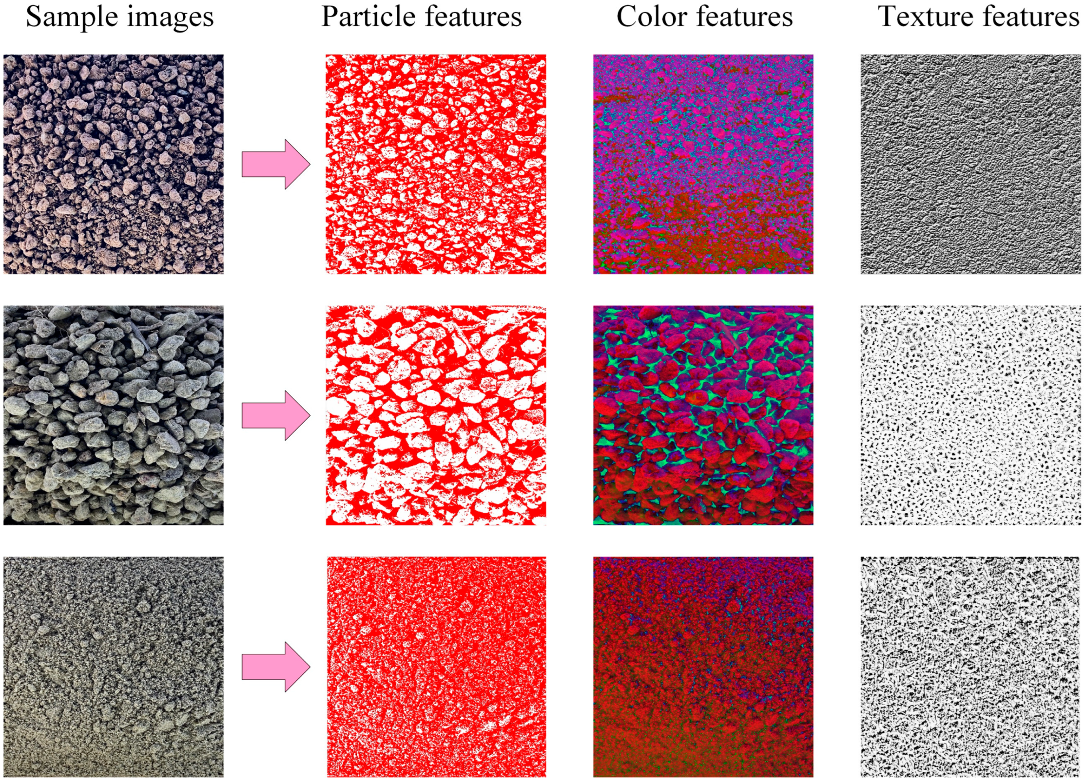
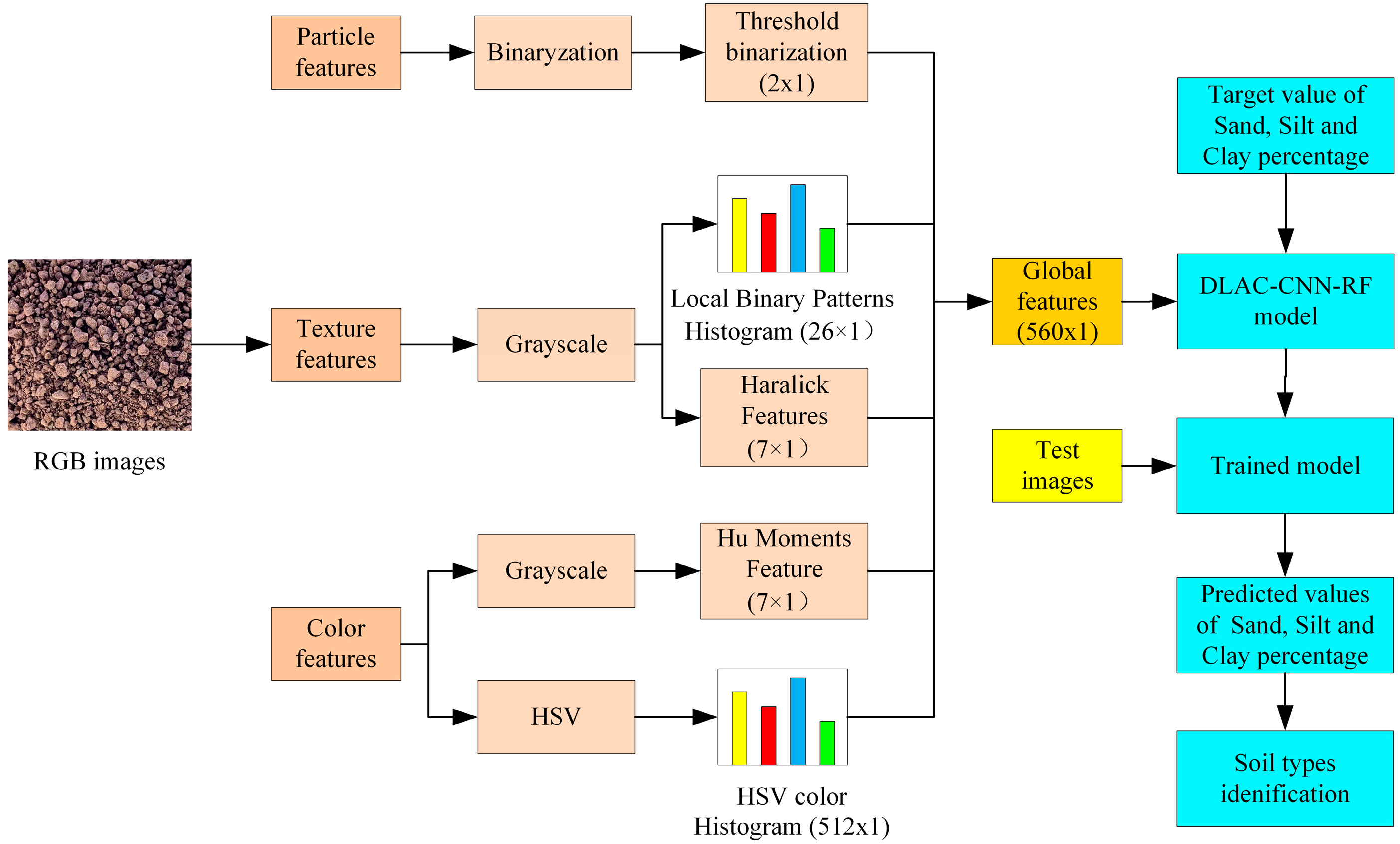
2.3. Image Feature Extraction

The physical properties of soil are typically characterized by colors and textures in the images. However, the particle features can also reflect the physical properties that need to be better investigated. In this work, a random combination of particle (Threshold binarization), color (HSV (hue, saturation, and value) and Hu moments), and textures features (Local binary patterns (LBP) and Haralick features) was extracted for soil image identification and classification, including particle, color, texture, particle + color, particle + texture, color + texture, and color + particle+ texture. Figure 3 reports the extracted particle, color, and texture features for silt, clay, and sand, respectively.

Figure 4 reports the flowchart of the processing of the extracted features for image identification. For threshold binarization, the OTSU threshold segmentation method was adopted; a threshold value of 120 and 2 channels were adjusted to transfer original soil particles to red in the images, which helps to calculate the soil particles area by reading the number of pixels. The RGB color of the sample images was converted into HSV components and reflected by a 512-dimension feature vector in HSV components. In addition, Hu moments are a set of 7 numbers calculated utilizing central moments that are constant under picture modifications. The LBP algorithm was used to characterize the texture feature of the soil images because it has been found to be an efficient approach to the traditional structural models of texture analysis. A ‘skimage’ package was used to generate the LBP histogram values through the texture, with a fixed number of 24 for circular symmetric neighbor set points and a radius of 8 pixels for each circle, producing 26 texture features. The Haralick feature algorithm was used to quantify an image according to its texture, and a total of 7 textural features were calculated for the following global features. Before particle, color, and texture features extraction, all the cropped soil images were processed into a grayscale image. A total of 554 global features were produced by particle (2 features), color (519 features), and texture (33 features), which were then imported into the proposed DLAC-CNN-RF model for further analysis.

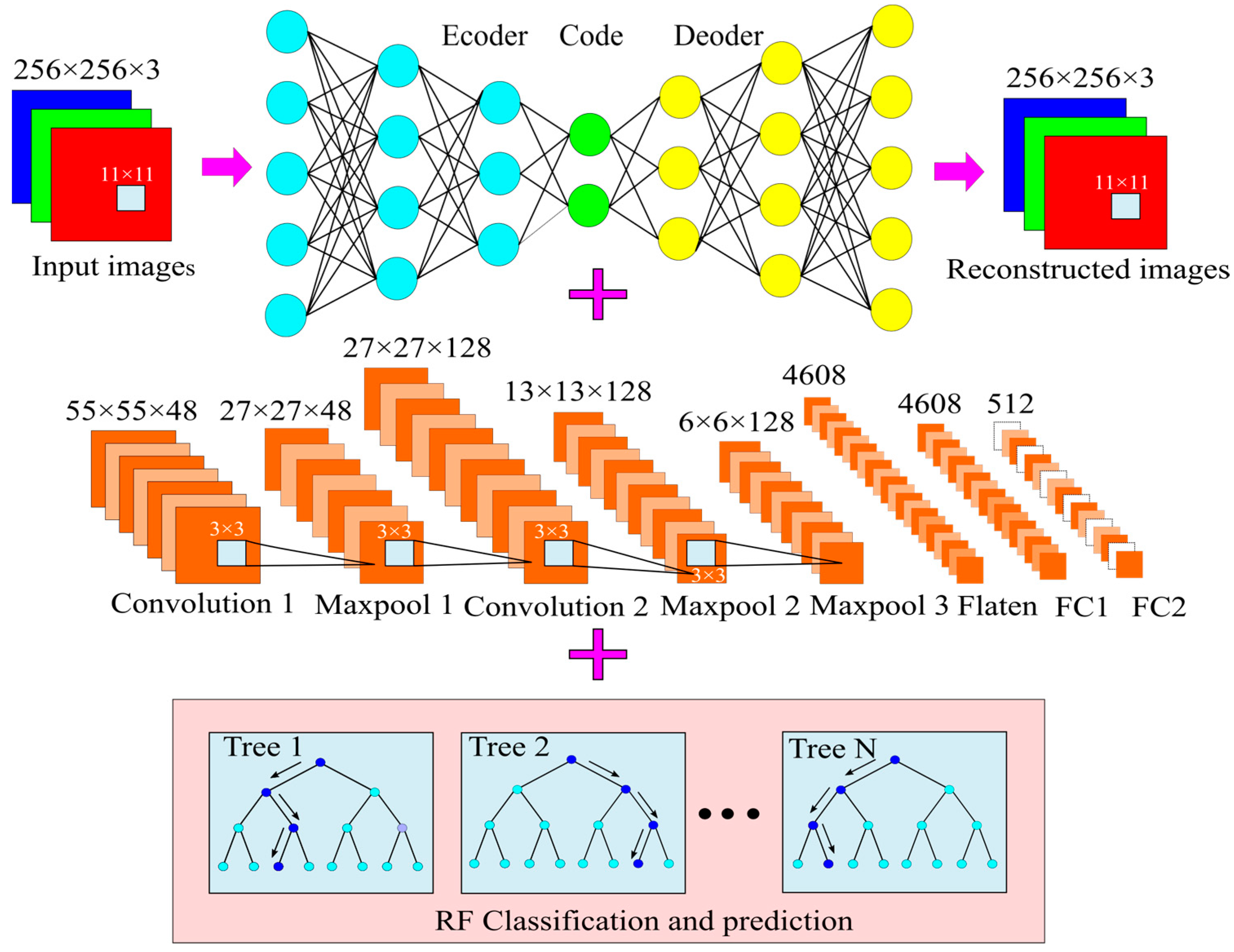
2.4. Developing a DLAC-CNN-RF Model

The DLAC is an excellent autoencoder that can be used for determining image properties since it incorporates probabilistic index extraction and process quantification in a general-purpose prediction system. A traditional autoencoder (AE) is trained to encode the input vector of image parameters x∈[0, 1], into a hidden representation y∈[0, 1]. The image characteristics are denoted as unlabeled data.

$${\left\{I_d\left[\left(N_{fx}{}^k,N_{fy}{}^k\right);\mu ,{\sigma }^2\right]\right\}}_{fx=1,fy=1}^{M_k,N_k}$$

(1)

so that the input can be reconstructed from that representation.

y = f_θ (x) = σ₁(Wx + b)

(2)

where f_θ(x) is called the encoder, θ = [W_x, b], W_x is a weight matrix, and b is a bias vector; σ₁ is a nonlinear activation function for the encoder. The resulted hidden representation y is then mapped back to a reconstructed vector z∈[0, 1]:

z = g_θ′      (y) = σ₂(W′y + b′)

(3)

where, g_θ′(y) is called the decoder of the image parameters, θ′ = [W′, b′] with appropriately sized parameters, σ₂ is a nonlinear activation function for the decoder. Here, DLAC takes the parametric input and encodes it to a linear representation of the soil characteristics. On the other side, the decoder takes hidden representations, passes them into nonlinearity, and generates the output of the probabilistic indexes.

$$L(x,z)=-{\displaystyle \sum _{k=1}^D(x_k\log z_k-(1-x_k)\log (1-x_k))}$$

(4)

DLAC tries to encode the parametric input stochastically applied to the input of the traditional autoencoder. It first uses a stochastic mapping $\tilde{x}\cong q_D(\tilde{x}\left|x\right.)$ to encode the parametric input into a hidden representation $y=f_{\theta }(\tilde{x})={\sigma }_1(W\tilde{x}+b)$ from which we reconstruct $z=g_{{\theta }^{\prime }}(\tilde{y})={\sigma }_2(W\tilde{y}+b^{\prime })$. Similar to a traditional autoencoder, the network weights are trained to minimize the average computation error, but the key difference is that z is now a deterministic function rather than x. Each layer of DLAC captures the complicated, higher-order correlations between the activities of the hidden features so that the input initialization can be utilized for the initial training of the input layer of the DLAC network.

Besides, the monitoring variables are divided into N labeled datasets: (x(1), y*(1)), (x(2), y*(2)),…, (x(N), y*(N)) and M unlabeled datasets: x(N + 1), x(N + 2),…, x(N + M), where M >> N, y is identified by the initial grinding or optimal soil value determinations. The correlation function of the intelligent prediction is defined as follows:

$$\begin{array}{l}\tilde{x},{\tilde{z}}^{(1)},\dots ,{\tilde{z}}^{(L)},\tilde{y}=g_{\theta \text{'}}(\tilde{x})\\ x,z^{(1)},\dots ,z^{(L)},y=g_{\theta }(\tilde{x})\\ \stackrel{⌢}{x},{\stackrel{⌢}{z}}^{(1)},\dots ,{\stackrel{⌢}{z}}^{(L)},\stackrel{⌢}{y}=W_{{\theta }^{\prime }}({\stackrel{⌢}{z}}^{(1)},\dots ,{\stackrel{⌢}{z}}^{(L)})\end{array}$$

(5)

In the forward path, individual layers of DLAC are formalized into linear transformations, then the nonlinear activation function is applied as

$${\tilde{h}}^{(l)}=Activation({\gamma }^{(l)}(z^{(l)}+{\beta }^{(l)}))$$

(6)

Here, h(l) is the postactivation function and W(l) is the weight matrix. The γ and β are the shifting and scaling parameters used before applying the nonlinearity function. The batch normalization is used to accelerate deep-learning network training. Finally, the prediction cost of DLAC is defined as

$$C(z^{(l)},{\widehat{z}}^{(l)})={‖\frac{{\widehat{z}}^{(l)}-{\mu }^{(l)}}{{\sigma }^{(l)}}-{\widehat{z}}^{(l)}‖}^2$$

(7)

where μ(l) and σ(l) are the mean and standard deviation of the encoder samples. This encoder is optimized by the objective correlation function to improve the accuracy of the intelligent prediction. In order to model each computation neutron coming out of the prediction network, generative adversarial network is used with competing behaviors for minimizing the training error and improving computational reliability. A successful DLAC training is one that gets to the same predictive cost and encoding function f_θ′(y). There is an error signal checking the similarity rate $y=f_{\theta }(\tilde{x})={\sigma }_1(W\tilde{x}+b)$. The training function for this network can be formulated as follows:

$$C(z,{\rho }^{(z)})=-E_{x~P_R(x)}[\log \gamma (l)]-E_{s~P_g}[\log (1-\sigma (z(l))]$$

(8)

Equally, the training function for E with setting parameters ρ(G) would be as follows:

$$C(\omega ,{\rho }^{(G)})=E_{S~P_R(S)}[\log (1-\rho ({\lambda }_{l}C({\tilde{z}}^{(l)}n)))]$$

(9)

Combining these functions into a single frame, both λ_l and z^(l)n would be trained and converge to a stable state of a Nash equilibrium. This means that the most optimal networks (generator and discriminator networks) could be reached as follows [25]:

$$\mathit{Cos}t=-{\displaystyle \sum _{n=1}^N\log P(\tilde{y}(n)=y*(n)\left|x(n)\right.)}+\omega {\displaystyle \sum _{n=N+1}^M{\displaystyle \sum _{l=1}^L{\lambda }_{l}C(z^{(l)}n,{\widehat{z}}^{(l)}n)}}$$

(10)

Here ỹ is the error output, y* is the true target, λ_l is the cost multiplier, which represents the weight of DLAC loss function for each decoding layer, and ω is a weight to balance different losses. This network illustrates different operational levels and data transmission in the architecture of DLAC. It could be learned that DLAC ranges across the measurement, calculation, and prediction levels. After training the first level of DLAC, the learned encoding function f_θ(y) is used on image parametric input x. Furthermore, a logistic regression layer can be added on the top of encoders to achieve a set of supervised network learning.

The established DLAC-CNN-RF model is shown in Figure 5. Soil images (256 × 256) are given as the inputs to the network and reconstructed by the autoencoders. Two convolution layers and three Maxpool layers were constructed to extract the image features. A flattened layer was used to transfer the 2D outputs of the max-pooling layer into 1D outputs. The convolution layers were connected to the Maxpool layers and attached to the full connected layers. Convolution 1 and 2 have a filter length of 48 and 128, respectively. A kernel function (11 × 11) was used for the layer of Convolution 1, while the remaining layers adopted the kernel function of 3 × 3. In particular, two max-pooling layers and two full connected layers were employed before and after the flattened layer to classify the extracted features. Finally, an RF model was employed to predict the soil types according to the random combination of image features. Among the 1000 soil image samples, 700 were used for training, and 300 samples were used for testing the network.

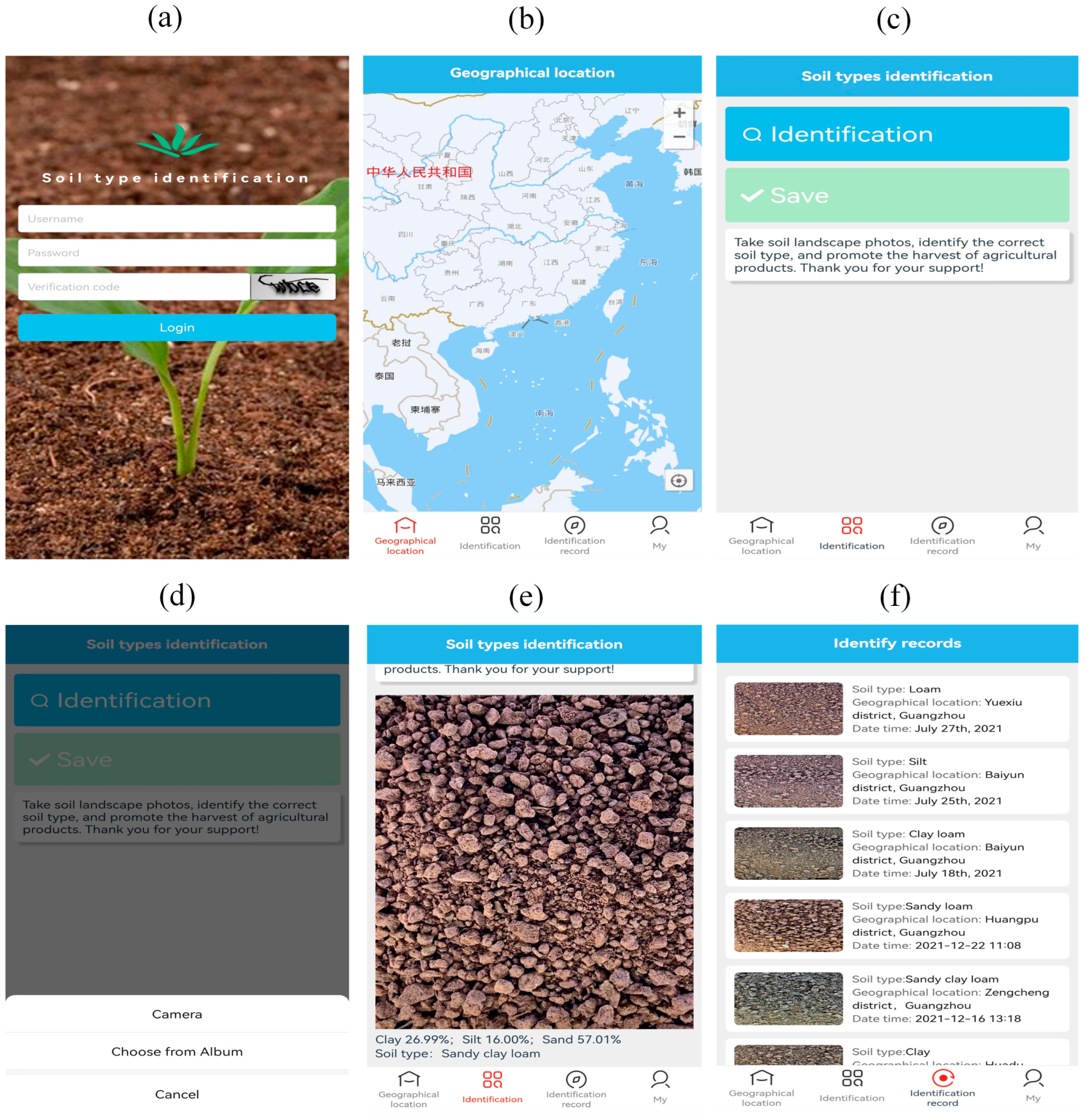
2.5. Developing a Graphical User Interface

An image recognition system named “Soil type identification” was developed based on basic Java programming language (JDK 1.8), where the pretrained DLAC-CNN-RF and RF model was deployed. A user-friendly interface was designed using Visual Studio Code software, as depicted in Figure 6. First, an account should be registered before logging into the system. After logging in, Baidu map was connected through an application programming interface, which helps to identify the geographical location of the input images. The input images can be selected from the camera or album. Once the image has been confirmed, the proposed DLAC-CNN-RF model responds quickly, as shown in Figure 5. The percentage of sand, clay, and silt was clearly presented in the interface, and the soil identification records were saved.

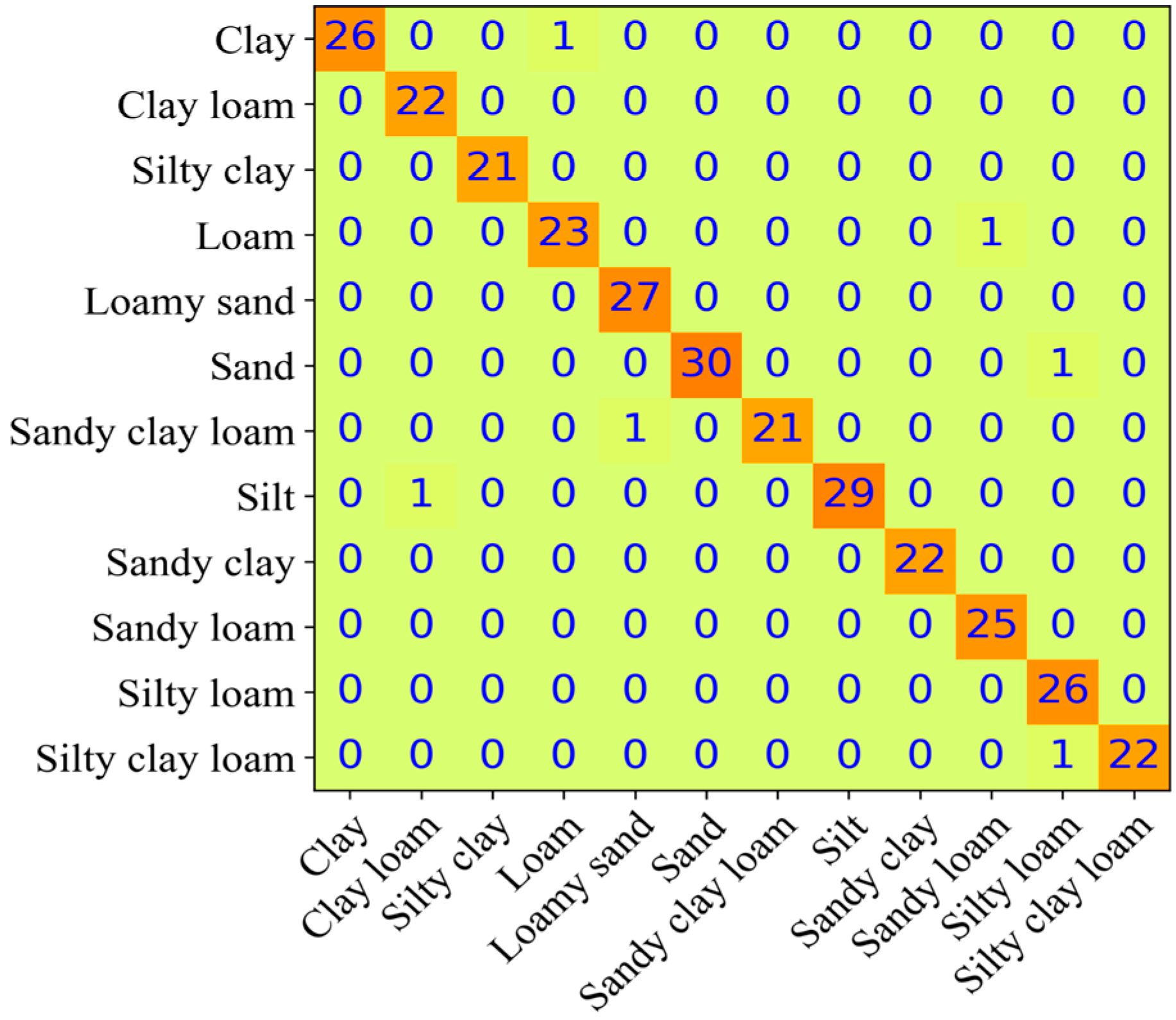
3. Results and Discussion

Figure 7 reports the average percentage of sand, silt, and clay in the prepared samples, which was measured via a hydrometer. The relationship of soil texture and the percentage of sand, silt, and clay was determined according to Stoke’s law [26]. The soil classification was based on USDA soil taxonomy [27]. It can be seen that the sand samples have the lowest silt and clay values, as well as the highest sand values with 3.5%, 6.1%, and 91.4%, respectively. The lowest sand values (10.3%) were obtained in the silt samples. Also, the sand, clay, and silt percentage dominated in the sand, clay, and silt samples, respectively.

Table 1. The RF and DLAC-CNN-RF model validation statistics for predicting clay, silt, and sand by using different combinations of image features. The number of the clay, silty clay, silty clay loam, sandy clay, sandy clay loam, clay loam, silt, silty loam, loam, sand, loamy sand, and sandy loam samples used for training were 58, 56, 53, 51, 56, 72, 53, 58, 57, 61, 61, and 54, respectively, and a total number of 700 was used.

	Extracted Feature	Model	MAE	RMSE	R2
Sand	Color	RF	3.67	4.44	0.95
		DLAC-CNN-RF	3.45	3.81	0.96
	Texture	RF	3.69	4.45	0.95
		DLAC-CNN-RF	3.48	3.85	0.96
	Particle	RF	3.74	4.53	0.94
		DLAC-CNN-RF	3.49	3.86	0.96
	Color + Texture	RF	3.58	4.35	0.96
		DLAC-CNN-RF	3.39	3.73	0.98
	Color + Particle	RF	3.62	4.37	0.96
		DLAC-CNN-RF	3.42	3.78	0.97
	Particles + Texture	RF	3.64	4.39	0.95
		DLAC-CNN-RF	3.44	3.80	0.97
	Color + Particle + Texture	RF	3.55	4.24	0.97
		DLAC-CNN-RF	3.37	3.71	0.99
Silt	Color	RF	3.81	4.46	0.79
		DLAC-CNN-RF	3.58	3.89	0.96
	Texture	RF	3.83	4.49	0.78
		DLAC-CNN-RF	3.59	3.94	0.94
	Particle	RF	3.89	4.57	0.73
		DLAC-CNN-RF	3.61	3.96	0.94
	Color + Texture	RF	3.73	4.40	0.85
		DLAC-CNN-RF	3.51	3.81	0.97
	Color + Particle	RF	3.74	4.43	0.82
		DLAC-CNN-RF	3.52	3.85	0.97
	Particles + Texture	RF	3.77	4.44	0.81
		DLAC-CNN-RF	3.55	3.88	0.96
	Color + Particle + Texture	RF	3.70	4.37	0.88
		DLAC-CNN-RF	3.48	3.79	0.98
Clay	Color	RF	3.68	4.68	0.93
		DLAC-CNN-RF	3.55	3.93	0.94
	Texture	RF	3.70	4.72	0.91
		DLAC-CNN-RF	3.48	3.84	0.97
	Particle	RF	3.74	4.75	0.90
		DLAC-CNN-RF	3.49	3.85	0.96
	Color + Texture	RF	3.63	4.61	0.97
		DLAC-CNN-RF	3.51	3.88	0.96
	Color + Particle	RF	3.64	4.65	0.95
		DLAC-CNN-RF	3.41	3.77	0.97
	Particles + Texture	RF	3.67	4.66	0.95
		DLAC-CNN-RF	3.45	3.81	0.98
	Color + Particle + Texture	RF	3.59	4.57	0.97
		DLAC-CNN-RF	3.46	3.83	0.98

reports the RF and DLAC-CNN-RF model validation statistics for predicting clay, silt, and sand using different extracted features. Obviously, the DLAC-CNN-RF model shows better performance in predicting soil textures due to a higher value of R². When the color feature is extracted, the RF and DLAC-CNN-RF model almost reach an agreement in predicting sand (i.e., R² 0.95 and 0.96) and clay (i.e., R² 0.93 and 0.94), while when predicting silt, a significant improvement was obtained in R² using the CCN-RF model. The value of R² improves from 0.79 to 0.96. Similarly, the DLAC-CNN-RF model gives obvious benefits to silt prediction when the texture and particle features were extracted; an R² value of 0.94 was obtained, while RF only realized an R² of 0.73. It’s noted that both the RF and DLAC-CNN-RF models show better performance in predicting sand and clay when a single image feature is extracted. This can be attributed to the fact that the average percentage of sand and clay in these samples is much more than that of silt. When multiple features were extracted, both the RF and DLAC-CNN-RF models showed progress in predicting all the soil textures. For sand and clay prediction, both the RF and DLAC-CNN-RF model show good performance when two features were extracted, although the DLAC-CNN-RF model is a little bit superior, while for silt prediction, the DLAC-CNN-RF model results in a higher R² value, with a 12~15% improvement in comparison to the RF model. Surprisingly, when the full features were extracted, the DLAC-CNN-RF mode exhibited an R² value of approximately 99% for all the soil textures. The better performance of the DLAC-CNN-RF model can be interpreted as a deeper study of the various edges, lines, and corners of the image. Notably, the validation RMSEs for predicting clay ranged from 3.71–3.86% among all the tested DLAC-CNN-RF models, which is a greater performance since clay typically shows a higher uncertainty in traditional measurements. This is mainly due to the use of extremely higher resolution cameras in smartphones. In addition, the established optimal networks (eq 10) offer a more quick and more efficient way than traditional autoencoders, which significantly reduce the noise of input data. Thus, the RMSEs values become lower.

Compared with the traditional method of predicting sand, soil, and clay, the proposed DLAC-CNN-RF model produces a better performance than that of Qi et al. [28] (R² values of 0.77, 0.68, and 0.71 for sand, silt, and clay, respectively) and Swetha et al. [23] (R² values of 0.97–98, 0.96–98, and 0.62–0.75 for sand, silt, and clay, respectively). The proposed method also exhibited a better prediction performance than Aitkenhead et al. [17] (R² values of 0.25, 0.19, and 0.18 for sand, silt, and clay, respectively). Additionally, this study showed a lower RMSE than Minasny et al. [29] (RMSE values of 6.31% and 6.23% for sand and clay, respectively).

Figure 8 reports the RF and DLAC-CNN-RF model predicted plots using full image features. In general, the proposed DLAC-CNN-RF mode shows higher accuracy in predicting all the soil types; the measured and predicted values are closer compared to the distribution in the RF models, especially for sand prediction, where the DLAC-CNN-RF model predicted value and measured value almost reach an agreement. Thus, the proposed DLAC-CNN-RF model appears to be preferable for predicting soil types.

The confusion matrix used for evaluating the performance of the DLAC-CNN-RF model is shown in Figure 9. The elements on the diagonal indicate that the predicted values equal the actual values, and these samples are classified correctly. The nonzero elements on the off-diagonal part of the matrix demonstrate a wrong classification. In most cases, the proposed model performs well in soil type identification. However, six images were classified incorrectly. For example, images in the clay, loam, sand, sandy clay loam, silt, and silty clay loam class were classified as loam, sandy loam, silty loam, loamy sand, clay loam, and silty loam, respectively.

Table 2. Performance parameters of the proposed DLAC-CNN-RF model for classification and prediction using full features. The number of the clay, silty clay, silty clay loam, sandy clay, sandy clay loam, clay loam, silt, silty loam, loam, sand, loamy sand, and sandy loam samples used for testing were 26, 23, 21, 24, 28, 30, 21, 29, 22, 26, 28, and 22, respectively, and a total number of 300 samples was employed.

Soil Textures	Accuracy	Precision	Sensitivity	Specificity	AUC
Clay	99.67%	100%	96.3%	100%	98.15%
Clay loam	99.67%	95.65%	100%	99.64%	99.82%
Silty loam	100%	100%	100%	100%	100%
Loam	99.33%	95.65%	95.83%	99.64%	97.74%
Loamy sand	99.67%	96.43%	100%	99.63%	99.82%
Sand	99.67%	100%	96.77%	100%	98.39%
Sandy clay loam	99.67%	100%	95.45%	100%	97.73%
Silt	99.67%	100%	96.67%	100%	98.34%
Sandy clay	100%	100%	100%	100%	100%
Sandy loam	99.67%	96.15%	100%	99.64%	99.82%
Silty loam	99.33%	92.86%	100%	99.28%	99.64%
Silty clay loam	99.67%	100%	95.65%	100%	97.83%
average	99.67%	98.06%	98.06%	99.82%	98.94%

shows the mean values of the classified performance parameters, including accuracy, precision, sensitivity, specificity, and area under the curve (AUC). An average accuracy of 99.67% was obtained using the proposed DLAC-CNN-RF model. The key parameters that determine the accuracy are sensitivity and specificity. Generally, the sensitivity parameter denotes how a model detects a positive sample, while specificity parameters show how a model detects negative samples. AUC describes an efficient relationship for evaluating the performance of the proposed DLAC-CNN-RF classifier model. A higher AUC value illustrates a better performance from the model. It is noted that the silty loam and sand clay were classified 100% correctly, and the ACU value for all predictions is over 97.5%.

Figure 10 reports the loss function of the proposed DLAC-CNN-RF model for training and testing the soil images. An epoch represents one cycle of updating the weights through the complete training soil image dataset. The loss value shows how well our model reacts after each iteration of optimization. A downward trend in the loss curves was observed, indicating the proposed model performs well for soil image classification.

Table 3. The comparison between the proposed DLAC-CNN-RF model and other models.

Model	Soil Types	Feature	Test
			R2	RMSE
KNN	Clay	Color + particle + texture	0.95	4.59
	Sand	Color + particle + texture	0.85	4.62
	Silt	Color + particle + texture	0.94	4.60
VGG16-RF	Clay	Color + particle + texture	0.85	4.23
	Sand	Color + particle + texture	0.93	3.85
	Silt	Color + particle + texture	0.97	3.95
Proposed DLAC-CNN-RF model	Clay	Color + particle + texture	0.99	3.76
	Sand	Color + particle + texture	0.99	3.71
	Silt	Color + particle + texture	0.98	3.79

shows the accuracy of the clay, sand, and silt soil image classifications of the proposed DLAC-CNN-RF model and other machine learning methods, including KNN and VGG16-RF. The full features of the prepared soil images were extracted in these models to evaluate their performance. As shown in Table 3, the conventional KNN model realizes an accuracy of 95% for clay image classification, which is relatively higher than the VGG16-RF models, but in terms of sand and silt classification, it is worse than the VGG16-RF model. In contrast, the proposed DLAC-CNN-RF model shows very good performance in classifying all the soil textures, exhibiting the highest R² and the lowest RMSE, which can be interpreted as the convolutional networks automatically and simultaneously extracting and selecting the features and reducing data over-fitting and complex computation.

4. Conclusions

This study demonstrated a cheap and environmentally friendly image acquisition system consisting of a smartphone, a customized chamber, and a mobile application for predicting soil images. The particle (threshold binarization), color (HSV (hue, saturation, and value) and Hu moments), and texture features (local binary patterns (LBP) and Harallick features) were extracted and used in random combinations to predict clay, silt, and sand content via RF and DLAC-CNN-RF algorithms. The results indicated that the proposed DLAC-CNN-RF model has better performance. Particularly, when the full features were extracted, an average accuracy of 99.67% was obtained when predicting all the soil textures. A user-friendly interface based on the calibrated DLAC-CNN-RF model has been designed, which clearly presents the prediction results. When compared with other commonly used models, the proposed DLAC-CNN-RF model is a promising solution that benefits from rapid and low-cost soil identification and classification. Our research may have two limitations. The first is that the used algorithm cannot predict soil moisture and organic carbon content. The second is the distance between the camera and the sample, which cannot be moved freely within the image acquisition system. Future research will study the effect of soil moisture and imaging distance on the prediction performance of the proposed model. Over the past few years, an unmanned aerial system (UAS)-based soil image acquisition method has received much attention due to its simple and fast implementation and the ability to take images with multiple elevation points in remote areas. Many UAS-based soil texture identification works have been reported [30,31,32]. Therefore, it is also worth exploring the classification and prediction performance of the proposed model by imputing images taken by the drone.

References

1. Phogat, V.K.; Tomar, V.S.; Dahiya, R. Soil physical properties. Soil Sci. Introd. 2015, 135–171. [Google Scholar]
2. Rahimi-Ajdadi, F.; Abbaspour-Gilandeh, Y.; Mollazade, K.; Hasanzadeh, R.P.R. Development of a novel machine vision procedure for rapid and non-contact measurement of soil moisture content. Measurement 2018, 121, 179–189. [Google Scholar] [CrossRef]
3. Klute, A. Methods of Soil Analysis. Part 1. Physical and Mineralogical Methods; Sssa book series 5; Soil Science Society of America: Madison, WI, USA, 1986. [Google Scholar]
4. Robinson, G.W. A new method for the mechanical analysis of soils and other dispersions. J. Agric. Sci. 1922, 12, 306–321. [Google Scholar] [CrossRef] [Green Version]
5. Di Stefano, C.; Ferro, V.; Mirabile, S. Comparison between grain-size analyses using laser diffraction and sedimentation methods. Biosyst. Eng. 2010, 106, 205–215. [Google Scholar] [CrossRef]
6. Chakraborty, S.; Weindorf, D.C.; Deb, S.; Li, B.; Paul, S.; Choudhury, A.; Ray, D.P. Rapid assessment of regional soil arsenic pollution risk via diffuse reflectance spectroscopy. Geoderma 2017, 289, 72–81. [Google Scholar] [CrossRef]
7. Fu, Y.; Taneja, P.; Lin, S.; Ji, W.; Adamchuk, V.; Daggupati, P.; Biswas, A. Predicting soil organic matter from cellular phone images under varying soil moisture. Geoderma 2020, 361, 114020. [Google Scholar] [CrossRef]
8. Andrenelli, M.C.; Fiori, V.; Pellegrini, S. Soil particle-size analysis up to 250 μm by x-ray granulometer: Device set-up and regressions for data conversion into pipette-equivalent values. Geoderma 2013, 192, 380–393. [Google Scholar] [CrossRef]
9. Fisher, P.; Aumann, C.; Chia, K.; O’Halloran, N.; Chandra, S. Adequacy of laser diffraction for soil particle size analysis. PLoS ONE 2017, 12, e0176510. [Google Scholar] [CrossRef] [Green Version]
10. Jaconi, A.; Vos, C.; Don, A. Near infrared spectroscopy as an easy and precise method to estimate soil texture. Geoderma 2019, 337, 906–913. [Google Scholar] [CrossRef]
11. Vaz, C.M.P.; de Mendonça Naime, J.; Macedo, Á. Soil particle size fractions determined by gamma-ray attenuation. Soil Sci. 1999, 164, 403–410. [Google Scholar] [CrossRef]
12. Vohland, M.; Ludwig, M.; Thiele-Bruhn, S.; Ludwig, B. Determination of soil properties with visible to near-and mid-infrared spectroscopy: Effects of spectral variable selection. Geoderma 2014, 223–225, 88–96. [Google Scholar] [CrossRef]
13. El Hourani, M.; Broll, G. Soil protection in floodplains—A review. Land 2021, 10, 149. [Google Scholar] [CrossRef]
14. Sofou, A.; Evangelopoulos, G.; Maragos, P. Soil image segmentation and texture analysis: A computer vision approach. IEEE Geosci. Remote Sens. Lett. 2005, 2, 394–398. [Google Scholar] [CrossRef]
15. Sudarsan, B.; Ji, W.; Adamchuk, V.; Biswas, A. Characterizing soil particle sizes using wavelet analysis of microscope images. Comput. Electron. Agric. 2018, 148, 217–225. [Google Scholar] [CrossRef]
16. Aitkenhead, M.; Coull, M.; Gwatkin, R.; Donnelly, D. Automated soil physical parameter assessment using smartphone and digital camera imagery. J. Imaging 2016, 2, 35. [Google Scholar] [CrossRef] [Green Version]
17. Aitkenhead, M.; Cameron, C.; Gaskin, G.; Choisy, B.; Coull, M.; Black, H. Digital rgb photography and visible-range spectroscopy for soil composition analysis. Geoderma 2018, 313, 265–275. [Google Scholar] [CrossRef]
18. de Oliveira Morais, P.A.; de Souza, D.M.; de Melo Carvalho, M.T.; Madari, B.E.; de Oliveira, A.E. Predicting soil texture using image analysis. Microchem. J. 2019, 146, 455–463. [Google Scholar] [CrossRef]
19. Breiman, L. Random forests. Mach. Learn. 2001, 45, 5–32. [Google Scholar] [CrossRef] [Green Version]
20. Dornik, A.; DrĂGuŢ, L.; Urdea, P. Classification of soil types using geographic object-based image analysis and random forests. Pedosphere 2018, 28, 913–925. [Google Scholar] [CrossRef]
21. Fan, R.; Bocus, M.J.; Zhu, Y.; Jiao, J.; Wang, L.; Ma, F.; Cheng, S.; Liu, M. Road crack detection using deep convolutional neural network and adaptive thresholding. In Proceedings of the 2019 IEEE Intelligent Vehicles Symposium (IV), Paris, France, 9–12 June 2019. [Google Scholar]
22. Vardhana, M.; Arunkumar, N.; Lasrado, S.; Abdulhay, E.; Ramirez-Gonzalez, G. Convolutional neural network for bio-medical image segmentation with hardware acceleration. Cogn. Syst. Res. 2018, 50, 10–14. [Google Scholar] [CrossRef]
23. Swetha, R.K.; Bende, P.; Singh, K.; Gorthi, S.; Biswas, A.; Li, B.; Weindorf, D.C.; Chakraborty, S. Predicting soil texture from smartphone-captured digital images and an application. Geoderma 2020, 376, 114562. [Google Scholar] [CrossRef]
24. Azadnia, R.; Jahanbakhshi, A.; Rashidi, S. Developing an automated monitoring system for fast and accurate prediction of soil texture using an image-based deep learning network and machine vision system. Measurement 2022, 190, 110669. [Google Scholar] [CrossRef]
25. He, R.; Dai, Y.; Lu, J.; Mou, C. Developing ladder network for intelligent evaluation system: Case of remaining useful life prediction for centrifugal pumps. Reliab. Eng. Syst. Saf. 2018, 180, 385–393. [Google Scholar] [CrossRef]
26. Gee, G.W.; Or, D. 2.4 particle-size analysis. Methods Soil Anal. Part 4 Phys. Methods 2002, 5, 255–293. [Google Scholar]
27. Soil Survey Staff. Soil Taxonomy: A Basic System of Soil Classification for Making and Interpreting Soil Surveys; USDA, Natural Resources Conservation Service: Washington, DC, USA, 1999.
28. Qi, L.; Adamchuk, V.; Huang, H.-H.; Leclerc, M.; Jiang, Y.; Biswas, A. Proximal sensing of soil particle sizes using a microscope-based sensor and bag of visual words model. Geoderma 2019, 351, 144–152. [Google Scholar] [CrossRef]
29. Minasny, B.; McBratney, A.B.; Tranter, G.; Murphy, B.W. Using soil knowledge for the evaluation of mid-infrared diffuse reflectance spectroscopy for predicting soil physical and mechanical properties. Eur. J. Soil Sci. 2008, 59, 960–971. [Google Scholar] [CrossRef]
30. Aboutalebi, M.; Allen, L.N.; Torres-Rua, A.F.; McKee, M.; Coopmans, C. Estimation of Soil Moisture at Different Soil Levels Using Machine Learning Techniques and Unmanned Aerial Vehicle (UAV) Multispectral Imagery; SPIE: Bellingham, WA, USA, 2019; pp. 216–226. [Google Scholar]
31. Marcu, I.; Suciu, G.; Bălăceanu, C.; Vulpe, A.; Drăgulinescu, A.-M. Arrowhead technology for digitalization and automation solution: Smart cities and smart agriculture. Sensors 2020, 20, 1464. [Google Scholar] [CrossRef] [Green Version]
32. Maimaitijiang, M.; Sagan, V.; Sidike, P.; Hartling, S.; Esposito, F.; Fritschi, F.B. Soybean yield prediction from uav using multimodal data fusion and deep learning. Remote Sens. Environ. 2020, 237, 111599. [Google Scholar] [CrossRef]
Figure 1. The location where the sample was collected.
Agronomy 12 03063 g001
Figure 2. The designed image acquisition device; (a) the constructed dark chamber from top view; (b) 3D view of the complete assembly.
Agronomy 12 03063 g002
Figure 3. The extracted image features from the soil samples for further processing.
Agronomy 12 03063 g003
Figure 4. Flowchart showing the image feature representation process applied to the captured images, including threshold binarization, local binary pattern histogram, Haralick features, Hu moments, and HSV color histogram.
Agronomy 12 03063 g004
Figure 5. The proposed DLAC-CNN-RF network architecture.
Agronomy 12 03063 g005
Figure 6. The running screen of the image recognition system for predicting soil texture: (a) the main menu; (b) the map of geographic location. Notably, the Chinese characters on the map represent different provinces in China, and the used Baidu map in this research only supports Chinese; (c,d) image selection; (e) DLAC-CNN-RF model predicted soil textural values; (f) identify records.
Agronomy 12 03063 g006
Figure 7. (a) The measured average percentage of clay, silt, and sand particles for clay, silty clay, silty clay loam, sandy clay, sandy clay loam, and clay loam, respectively; (b) the measured average percentage of clay, silt, and sand particles for silt, silty loam, loam, sand, loamy sand, and sandy loam, respectively; the number of samples counted for clay, silty clay, silty clay loam, sandy clay, sandy clay loam, clay loam, silt, silty loam, loam, sand, loamy sand, and sandy loam are 84, 79, 74, 75, 84, 102, 74, 97, 79, 87, 89, and 76, respectively.
Agronomy 12 03063 g007
Figure 8. The measured and predicted plots for (a) sand, using full features (RF), (b) sand, using full features (DLAC-CNN-RF), (c) clay, using full features (RF), (d) clay, using full features (DLAC-CNN-RF), (e) silt, using full features (RF), and (f) silt, using full features (DLAC-CNN-RF).
Agronomy 12 03063 g008
Figure 9. Predicted distributions of 12 soil textures classes via the proposed DLAC-CNN-RF model.
Agronomy 12 03063 g009
Figure 10. Classification accuracy and error rate using the proposed DLAC-CNN-RF model for (a) sand images, (b) clay images, and (c) silt images.
Agronomy 12 03063 g010