Efficient Identification of Apple Leaf Diseases in the Wild Using Convolutional Neural Networks

Abstract

Efficient identification of apple leaf diseases (ALDs) can reduce the use of pesticides and increase the quality of apple fruit, which is of significance to smart agriculture. However, existing research into identifying ALDs lacks models/methods that satisfy efficient identification in the wild environment, hindering the application of smart agriculture in the apple industry. Therefore, this paper explores an ACCURATE, LIGHTWEIGHT, and ROBUST convolutional neural network (CNN) called EfficientNet-MG, improving the conventional EfficientNet network by the multistage feature fusion (MSFF) method and gaussian error linear unit (GELU) activation function. The shallow and deep convolutional layers usually contain detailed and semantic information, respectively, but conventional EfficientNets do not fully utilize the different stage convolutional layers. Thus, MSFF was adopted to improve the semantic representation capacity of the last layer of features, and GELU was used to adapt to complicated tasks. Further, a comprehensive ALD dataset called AppleLeaf9 was constructed for the wild environment. The experimental results show that EfficientNet-MG achieves a higher accuracy (99.11%) and fewer parameters (8.42 M) than the five classical CNN models, thus proving that EfficientNet-MG achieves more competitive results on ALD identification.

1. Introduction

Apples (Malus × domestica Borkh.) are rich in many vitamins and provide material security for human health. Meanwhile, the apple industry is one of the largest fruit industries in the world [1,2]. With the advent of COVID-19, securing the world’s food supply has become even more critical. However, due to plant leaf diseases, apples may suffer significant quality deterioration and yield losses. For example, scab, one of the typical apple diseases, is highly contagious and can cause yield losses of 70% or more if not appropriately managed [2]. One of the typical applications of artificial intelligence (AI) in agriculture is the automatic identification of crop diseases. Smart agriculture requires unmanned aerial vehicles (UAVs) to diagnose crop diseases accurately and apply pesticides in real time [3,4]. At the same time, farmers can make precise diagnoses of plant diseases via their mobile phones. However, traditional apple leaf disease (ALD) identification methods mainly rely on expert experience to manually extract features such as the texture, shape, and color of the diseased leaf images [5]. Due to the complexity of the disease spots and background, the manual identification process is often laborious, time-consuming, and subjective [6]. Therefore, efficient identification of ALDs can reduce the use of pesticides and increase the yield of apple fruit, which is of significance to environmental protection and the apple industry.

With the development of traditional machine learning (ML) methods, some identification methods for plant diseases have been proposed. Chuanlei et al. adopted a genetic algorithm and correlation-based feature selection to select the most valuable features of the 38 types of features. They then used a support vector machine (SVM) classifier to identify three categories of ALDs, with which they were able to achieve 94.22% accuracy [7]. Singh et al. applied the brightness-preserving dynamic fuzzy histogram equalization technique to enhance images and then used the k-nearest neighbor (KNN) classifier to identify two categories of ALDs. In their experimental results, the classification accuracy was 96.41% [8]. Although traditional ML makes the diagnosis of plant diseases more convenient, the feature extraction of these plant diseases is artificially designed. Extracting features through artificial designs is often laborious and time-consuming.

In recent years, increasing speeds and capacities of graphical processing units (GPUs) have paved the way for the development of convolutional neural networks (CNNs) [9]. Researchers have applied CNN models to smart agriculture with encouraging results. Zhong and Zhao utilized a CNN model based on the DenseNet-121 [10] network and compared three methods of the classification loss function to identify ALDs. In their experimental results, the best accuracy was 93.71% [11]. However, the dataset for their experiment did not contain images in the wild environment. Yadav and Yadav presented a CNN model that applies a fuzzy c-means clustering algorithm and a contrast stretching-based preprocessing technique to identify ALDs. Although their proposed model achieved 98% accuracy, it can only identify four categories of ALDs [12]. To identify four categories of ALDs, Jiang et al. used a CNN model using the ResNet [13] network and the transfer learning algorithm. Their experiment results showed that the ALD identification accuracy of their model is 83.75%. Although the accuracy of their proposed model exceeded that of the traditional ResNet model, the model was not designed to be lightweight [14]. Chao et al. implemented global average pooling (GAP) [15] layers instead of fully connected (FC) layers and proposed a CNN model named XDNet, which combined DenseNet [10] and Xception [16]. Their proposed model achieved 98.82% accuracy on a dataset containing healthy leaves and five categories of ALDs [17]. In another study, Bi et al. proposed an improved CNN model based on MobileNet [18] for ALD identification. Although his proposed model is lightweight, it only obtained 73.50% recognition accuracy for two types of ALDs [19]. Yan et al. adopted an improved model based on VGG [20] for ALD identification in which batch normalization (BN) [21] layers were adopted to improve the inference speed. Meanwhile, the GAP layer was used to replace the FC layer to reduce parameters (params). They tested on the PlantVillage dataset (PVD) [22] and obtained 99.01% classification accuracy [23]. Luo et al. utilized BN layers and the rectifier linear unit (ReLU) activation function to improve ResNet. To solve the severe loss of information in the ResNet downsample, they used channel projection and spatial projection of downsampling. Their proposed method achieved 94.99% accuracy on a dataset containing five types of ALDs and healthy leaves. However, this model had more than 20 M parameters which made it challenging to meet the needs of mobile devices [24]. Yu et al. proposed the MSO-ResNet (multistep optimization ResNet) network as an ALD recognition model. To reduce the parameters of their proposed model, they presented the convolution kernel decomposition and the identity mapping methods. Their proposed model achieved an average of 95.70% accuracy [25]. Recently, Pradhan et al. utilized ten well-known CNN models for the detection of ALDs. In their experiments, the dataset consisted of three classes of ALDs and healthy leaves from PVD. Their experiments showed that DenseNet-201 [10] outperformed the other nine CNN models with an accuracy of 98.75% [26]. In addition, Gao et al. proposed a CNN to assess the severity of Fusarium head blight (FHB) in wheat. By calculating the proportion of the diseased area to the total area, the disease degree of wheat FHB was divided into four levels, and the accuracy of disease level prediction reached 91.8% [27].

Despite the research mentioned above on breakthroughs in CNN applications for smart agriculture, there are still some shortcomings in the existing research, such as the lack of accurate and lightweight CNN models for mobile devices. Efficient identification means that CNNs can achieve high-precision identification with fewer params. In terms of datasets for identifying ALDs, there is a lack of datasets with rich categories in the wild environment. A wild environment means the background of plant leaves in the image, not the static background in the laboratory (usually a single-color background), but the real natural wild background. Agricultural practitioners use mobile phones to diagnose plant diseases accurately, usually in non-laboratory environments. Typically, the average execution time (AET) indicates the inference time required to predict a given image. Keeping a lower AET and fewer parameters is beneficial for the deployment of mobile devices. Therefore, this study aims to explore a novel ALD identification model to compensate for the inefficiency of the models proposed in existing studies. Meanwhile, a category-rich ALD dataset was constructed to make up for the shortcomings of the existing ALD dataset with fewer categories. The contributions of this paper are summarized as follows:

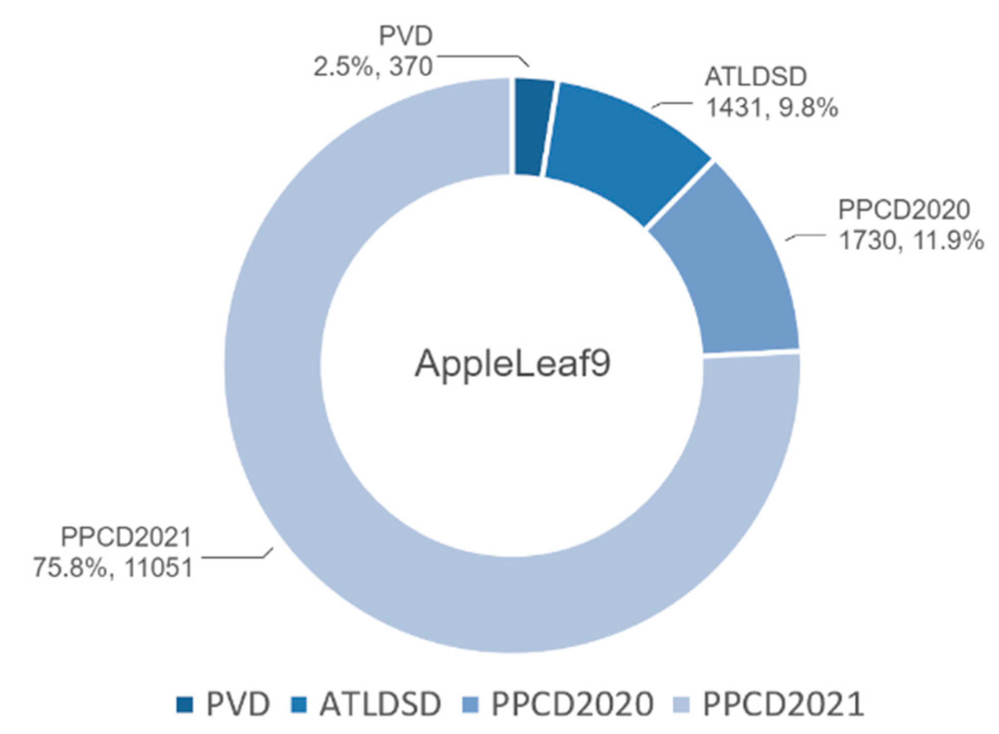
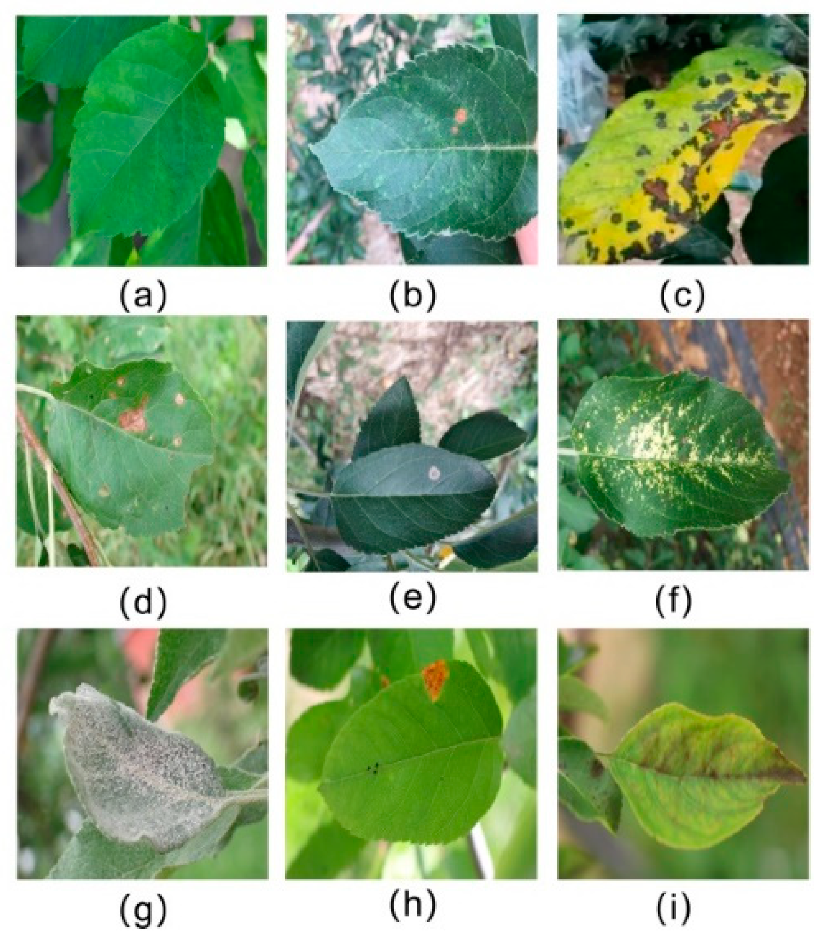
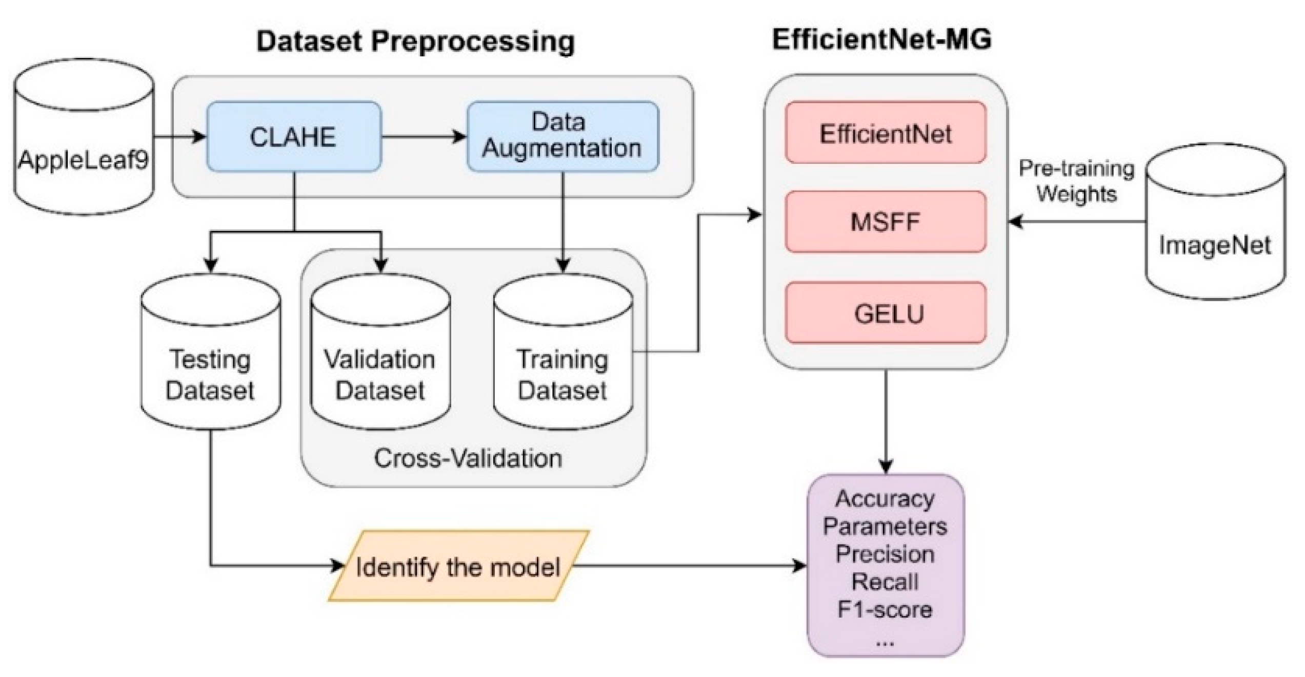
• Data fusion: An apple leaf disease dataset called AppleLeaf9 was constructed to ensure the generalization of performance of the CNN model. To improve the diversity of the identified categories, AppleLeaf9 fuses together four different ALD datasets. The AppleLeaf9 dataset includes healthy apple leaves and eight categories of ALDs, most of which are in the wild environment.
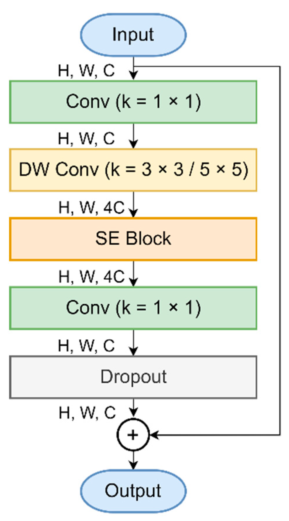
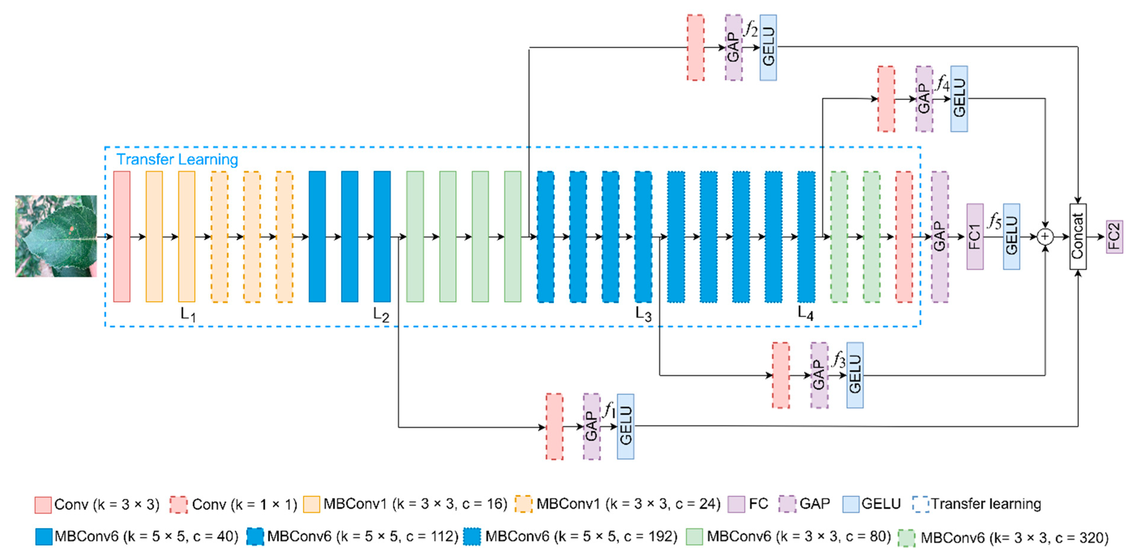
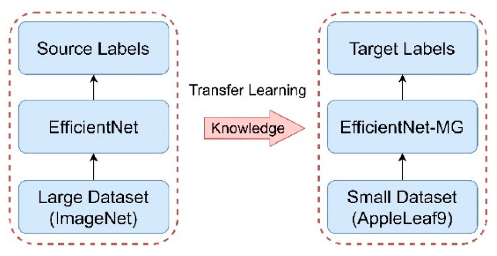
• A novel ALD identification model called EfficientNet-MG is proposed. This model introduces the multistage feature fusion (MSFF) method and the Gaussian error linear unit (GELU) activation function into EfficientNet, which has the following three merits:

Accurate: Compared to classical CNN models and previous research methods, the proposed model ensures a higher accuracy in ALD identification;

Lightweight: To meet real-time demands on mobile devices, the proposed model maintains a lower AET and fewer parameters;

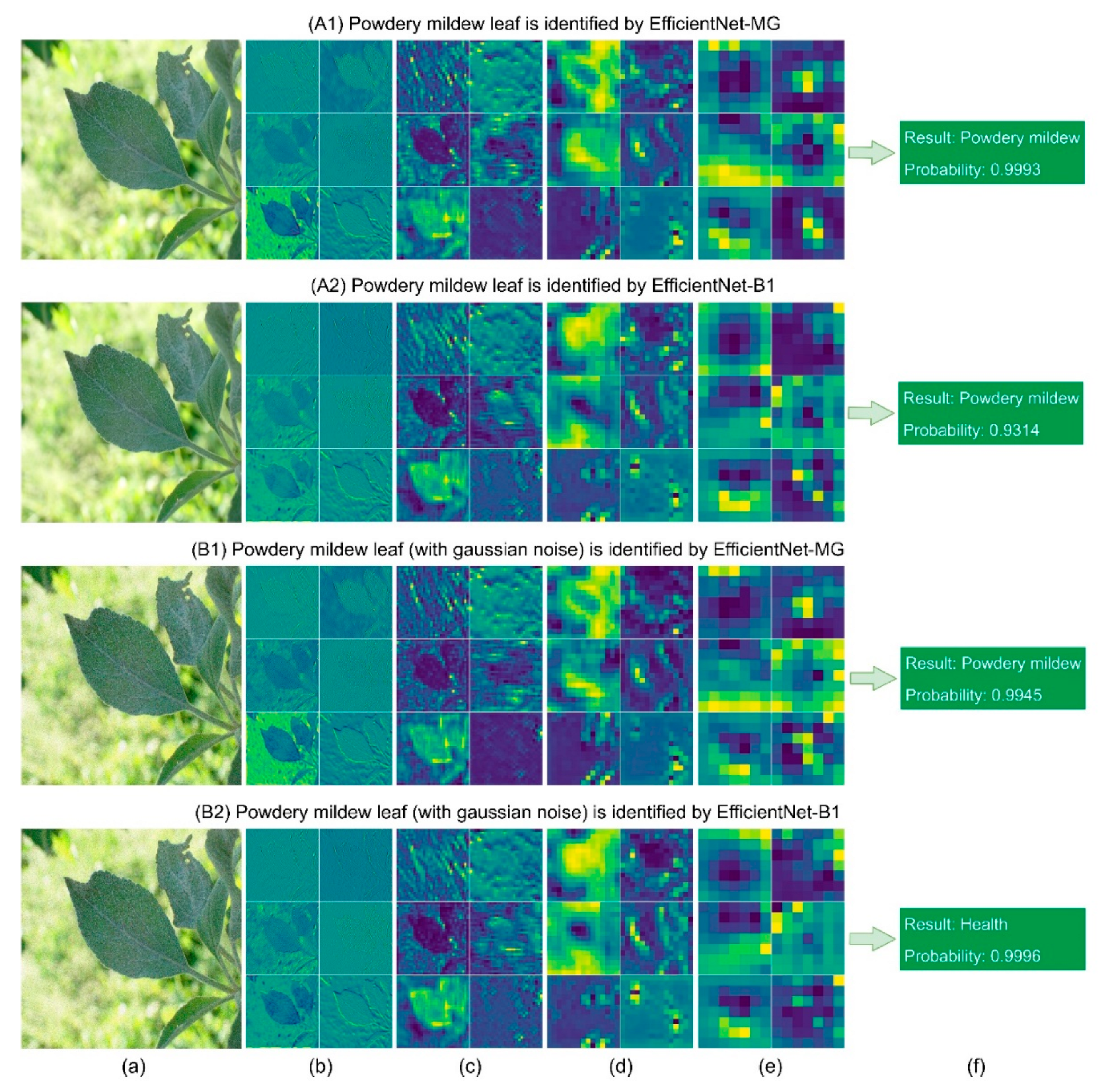
Robust: More types of ALDs can be identified in the wild environment without limiting the shooting angles, noise, and other factors.

The rest of this paper is organized as follows: Section 2 describes the datasets and EfficientNet-MG. Experimental studies are given in Section 3. In Section 4, the results and comparisons with classical models are obtained. Discussions with comparative research are given in Section 5. Finally, this paper is concluded in Section 6.

2. Materials and Methods

In this section, the comprehensive dataset called AppleLeaf9 is first introduced. Second, the preprocessing image strategy is described, such as contrast limited adaptive histogram equalization (CLAHE) and data augmentation methods. Finally, EfficientNet-MG is presented, including the EfficientNet network, MSFF method, GELU activation function, and transfer learning strategy.

2.1. AppleLeaf9

Insufficient data and low regional representations are among the main issues affecting the performance of the prediction models [28]. PVD collected 54,306 images of 14 crop species with 26 diseases, and it contained healthy apple leaves and three categories of ALDs [22]. However, PVD only contained static background images. It was necessary to collect ALD images with wild backgrounds to meet the needs of the natural field environment [17]. The plant pathology challenge datasets (PPCD2020, PPCD2021) were taken from the online data science platform Kaggle, and the images were collected in wild fields [29]. The apple tree leaf disease segmentation dataset (ATLDSD) was collected from four different apple experimental demonstration stations. ATLDSD was collected in the laboratory (about 51.9%) and wild fields (about 48.1%) under different weather conditions [30].

The fusion of the four datasets can make the proposed model identify more categories of ALDs in the wild environment, which enhances the model’s ability to cope with environmental changes, thus making the proposed model more robust. Therefore, in this paper, the dataset called AppleLeaf9 was fused from PVD, ATLDSD, PPCD2020, and PPCD2021. The AppleLeaf9 dataset is available at https://github.com/JasonYangCode/AppleLeaf9 (accessed on 7 October 2022). AppleLeaf9 will help agricultural practitioners better apply CNN models to solve more ALD practical problems. Agricultural disease experts were invited to screen each image, and images with incorrect labels were removed. In the process of data fusion, some static background images were reduced. Since PVD contains only static background images, only 2.5% of all images in AppleLeaf9 are from PVD. At the same time, since some disease categories of ATLDSD, PPCD2020, and PPCD2021 are the same, AppleLeaf9 fuses partial images of the three datasets. The AppleLeaf9 dataset contains 14,582 images, 94% in the wild environment. The distribution of AppleLeaf9’s image sources is shown in Figure 1.

The dataset of AppleLeaf9 includes healthy apple leaves and eight categories of ALDs, with the main symptoms and causes shown in

Table 1. Main symptoms and causes of the eight types of ALDs.

Types	Main Symptoms	Main Causes
Alternaria leaf spot	The diseased spots often have small round brown or black lesions that gradually enlarge with a brownish-purple border on leaves.	Alternaria alternata f. sp. mali
Brown spot	The dark brown spots are morphologically different from other lesions.	Marssonina coronaria
Frogeye leaf spot	The center of the spot turns brownish with dark-brown to purplish edges, giving the spot a frog eye appearance.	Botryosphaeria obtusa
Grey spot	In the early stages, sub-circular yellow-brown lesions are found, which later turn grey.	Phyllosticta pirina Sacc. & Coryneum foliicolum
Mosaic	Bright yellow spots spread throughout the leaves.	Apple mosaic virus
Powdery mildew	Tiny white spots spread throughout the leaves.	Podosphaera leucotricha
Rust	The diseased spots are often rusty yellow dots with brown acicular dots in the center of these dots.	Pucciniaceae glue rust
Scab	The diseased spots are velvet-like with fringed borders.	Venturia inaequalis

[1,17,28]. The samples of AppleLeaf9 are shown in Figure 2. In the early stages of grey spot, subcircular yellow-brown lesions are found. Then, the spot turns grey. Therefore, Alternaria leaf spot is easily confused with grey spot in its early stage, which raises the difficulty of identifying the two spots.

2.2. Dataset Preprocessing

2.2.1. CLAHE

CLAHE has been proposed and summarized [31,32]. This technique, which has been successfully proven to be effective in biomedical image analyses [33], is an adaptive contrast histogram equalization method. The contrast of an image is reinforced by applying contrast limited histogram equalization (CLHE) on small image areas, called tiles, rather than the entire image. In addition, CLAHE reduces the noise amplification of the tiles by limiting the contrast. Although it does not eliminate artifacts, it is better than adaptive histogram equalization (AHE).

The process of CLAHE can be divided into three steps. Firstly, the image is decomposed into rectangular blocks of equal size, and histogram adjustment is performed in every rectangular block, including histogram creation, clipping, and redistribution. Secondly, the mapping function is obtained by the cumulative distribution function of the clipped histogram. Finally, bilinear interpolation between the rectangular blocks is used to remove possible block artifacts. The histogram statistics comparison between the original and CLAHE images is shown in Figure 3. The grayscale value is a constrained linear combination of the red (R), green (G), and blue (B) channels of the input color image. The weights of R, G, and B are 0.299, 0.587, and 0.114, respectively, and their summation is 1. It can be seen that the details of the leaf disease spots become clearer after using CLAHE, and the pixels of the greyscale image are more widely distributed on the X-axis.

2.2.2. Data Augmentation

One of the main features of CNNs is their generalization ability, that is, their ability to process data that has never been observed. However, when the data diversity is limited, CNN models tend to overfit and have a low generalization ability after training [34]. The AppleLeaf9 dataset has been divided into three subsets, including training, validation, and testing datasets in a ratio of 3:1:1. To improve the network’s generalization ability and reduce overfitting, the data augmentation methods were randomly used to simulate the changes in angle and noise. The total number in the training dataset was increased one time to 17,512 images after the data augmentation. Examples of dataset augmentation are shown in Figure 4, where the direction of rotation is counterclockwise. The number of images in the dataset is recorded in

Table 2. Number of images for training, validation, and testing.

Types	Total Images	Training Images		Validation Images	Testing Images	Labels
		Original	Augmentation
Alternaria leaf spot	417	251	502	83	83	A1
Brown spot	411	247	494	82	82	A2
Frogeye leaf spot	3181	1909	3818	636	636	A3
Grey spot	339	205	410	67	67	A4
Healthy	516	310	620	103	103	A5
Mosaic	371	223	446	74	74	A6
Powdery mildew	1184	712	1424	236	236	A7
Rust	2753	1653	3306	550	550	A8
Scab	5410	3246	6492	1082	1082	A9
Sum	14,582	8756	17,512	2913	2913	-

.

2.3. Proposed EfficientNet-MG

2.3.1. EfficientNet

As the CNNs used in the ImageNet dataset have become more complex since 2012, the accuracy has continued to increase, but many models are not effective in computational load. Tan and Le proposed EfficientNet, one of the state-of-the-art models, achieving an accuracy of 84.3% in the ImageNet dataset and can be regarded as a group of CNN models [35]. The EfficientNet group consists of 8 models between B0 and B7 derived from the baseline network (usually called EfficientNet-B0) by extension. The advantages of EfficientNet are reflected in two aspects: it not only has a higher accuracy, but also improves the model’s effectiveness by reducing parameters and floating-point operations (FLOPs) [36]. Unlike other CNN models, EfficientNet uses a new activation function called SiLU instead of the ReLU activation function.

By adopting the network architecture search (NAS) method in all network dimensions (i.e., width, depth, and resolution), EfficientNet has attracted attention because of its advantages in predictive performance. The width refers to the number of channels in any layer, the depth relates to the number of layers, and the resolution is associated with the size of the images. The dimensions are scaled in the following way through composite coefficients:

$$\begin{gathered} \mathrm{depth}:d={\alpha }^{\phi } \\ \mathrm{width}:w={\beta }^{\phi } \\ \mathrm{resolution}:r={\gamma }^{\phi } \\ \mathrm{s}.\mathrm{t}.\alpha ·{\beta }^2·{\gamma }^2\approx 2 \\ \alpha \ge 1,\beta \ge 1,\gamma \ge 1 \end{gathered}$$

(1)

where $\phi$ is a composite coefficient and $\alpha$, $\beta$, and $\gamma$ are the scaling coefficients of each dimension that the grid search can fix. After determining the scaling coefficients, these coefficients are applied to the baseline network (EfficientNet-B0) for scaling to obtain the desired target model size and parameters. For example, in the case of EfficientNet-B0, when $\phi$ = 1 is set, the optimal values are yielded by grid search, i.e., $\alpha$ = 1.2, $\beta$ = 1.1, and $\gamma$ = 1.15, under the constraint of $\alpha ·{\beta }^2·{\gamma }^2\approx 2$. By changing the value of $\phi$ in Equation (1), EfficientNet-B0 can be enlarged to obtain EfficientNet-B1 to B7.

Table 3. EfficientNet-B0 network structure of the baseline network.

Stage	Operator	Resolution	Channels	Layers
1	Conv3×3	224 × 224	32	1
2	MBConv1, k = 3 × 3	112 × 112	16	1
3	MBConv6, k = 3 × 3	112 × 112	24	2
4	MBConv6, k = 5 × 5	56 × 56	40	2
5	MBConv6, k = 3 × 3	28 × 28	80	3
6	MBConv6, k = 5 × 5	14 × 14	112	3
7	MBConv6, k = 5 × 5	14 × 14	192	4
8	MBConv6, k = 3 × 3	7 × 7	320	1
9	Conv1×1 & Pooling & FC	7 × 7	1280	1

showcases the network structure of EfficientNet-B0, in which k is the size of convolution kernels.

The feature extraction blocks of EfficientNet consist of mobile reverse bottleneck convolution (MBConv) [37] blocks, with built-in convolution (conv), BN, SiLU, depth-wise convolution (DW Conv), squeeze-and-excitation (SE) [38] blocks, and dropout. The structure of the MBConv block is illustrated in Figure 5, where H, W, and C represent the height, width, and channel size of the feature map, respectively. In the MBConv block, the input channel size is first expanded by a factor of four and then the four-times-wider state is projected back to the original channel size.

2.3.2. MSFF Method

Recent studies have demonstrated that it is worth employing CNN features from multiple stages since the shallow convolutional layers contain detailed information, and the deep convolutional layers have rich semantic information [39]. Although EfficientNet uses the NAS method and MBConv blocks, the different stage convolutional layers were not fully utilized. Therefore, the MSFF method is used to learn complementary information from multiple-stage convolutional layers to address this problem.

Due to the need for being lightweight, EfficientNet-B1 is adopted as the baseline network to integrate the features of different stage convolutional layers. The features of various layers $f_1$ are complementary to improve the semantic representation capacity of the last layer of features. The neural network architecture of EfficientNet-MG is depicted in Figure 6, in which k and c represent the size and number of convolution kernels, respectively. The GAP layers are used in EfficientNet-MG to replace part of the FC layers to reduce parameters and suppress overfitting.

Due to the features of different layers having different influencing factors, $\mathrm{GELU}\left(f_1\right)$ is prefixed with the weighting factor ${\lambda }_i$. The MSFF formula of EfficientNet-MG is shown in Equation (2). For comparative analysis, EfficientNet-MG1 to MG3 are proposed as alternative models with the formulas shown in Equations (3)–(5).

$$f_{MG}=\mathrm{Concat}\left(\mathrm{GELU}\left(f_1\right),\mathrm{GELU}\left(f_2\right),{\displaystyle \sum }_{i=3}^5{\lambda }_i\mathrm{GELU}\left(f_i\right)\right)$$

(2)

$$f_{MG1}={\displaystyle \sum }_{i=3}^5{\lambda }_i\mathrm{GELU}\left(f_i\right)$$

(3)

$$f_{MG2}={\displaystyle \sum }_{i=3}^5\mathrm{GELU}\left(f_i\right)$$

(4)

$$f_{MG3}=\mathrm{Concat}\left(\mathrm{GELU}\left(f_1\right),\mathrm{GELU}\left(f_2\right),\cdots ,\mathrm{GELU}\left(f_5\right)\right)$$

(5)

2.3.3. GELU Activation Function

The activation function choice is a necessary architecture decision for CNNs to prevent the network as a deep linear classifier. Therefore, the activation functions play an essential role in CNNs for complex tasks. The activation function of ReLU, which has been extensively applied in CNNs, was proposed to realize better object recognition. To further enhance the capability of ReLU, the activation function of exponential linear unit (ELU) [40] was developed in 2015. After that, the activation function of SiLU was found to realize a smooth, non-monotonic function. The GELU activation function is a high-performing activation function [41]. Its nonlinearity weights inputs by their value, rather than gating inputs by their sign, as in ReLU. Since the GELU activation function has superior performance [42,43], it was adopted by EfficientNet-MG to accommodate complex identification tasks. Considering that the transfer learning strategy is applied to EfficientNet-MG, this paper uses GELU in part of the FC layers.

2.4. Transfer Learning

CNNs usually require training in many annotated images to achieve a high prediction accuracy. However, obtaining such a large-scale dataset is difficult and expensive. In response to these challenges, many previous studies have adopted transfer learning methods to solve cross-domain image classification problems, and they have proven to be very useful [17,23,26]. The transfer learning method is an ML method in which the knowledge gained during training in a task is used for training in another field [44]. In the real world, some examples can be used to explain the transfer learning method. For example, learning to play the electronic organ may help us understand the piano [44]. Undersampling of the dataset can easily cause overfitting problems in training, which will lead to poor robustness of the model. Using pretrained model weights built on the ImageNet dataset (involving 3.2 million images), EfficientNet-MG was optimized by the transfer learning method. Figure 7 showcases the transfer learning process from the EfficientNet network to EfficientNet-MG [45].

3. Experiment

In this section, the experimental setup is first introduced, including details of the testing platform and hardware. Then, the training settings (including the loss function, optimizer, and dynamic multistage attenuation learning rate (DMALR)) are presented, where four-fold cross-validation is used to ensure the reliability of the experiments. Finally, the details of the performance metrics are provided. The block diagram of the experimental procedure is illustrated in Figure 8.

3.1. Experimental Device

All CNN models used in this work were compiled with a GPU and Python language support. The experimental studies were conducted in the TensorFlow deep learning (DL) framework and the Ubuntu server. The configuration parameters of the experiments are recorded in

Table 4. Hardware and software environment.

Configuration	Value
GPU	NVIDIA GeForce RTX 3080 Ti 12 GB (NVIDIA Inc., Santa Clara, CA, USA)
CPU	12th Gen Intel(R) Core(TM) i7-12700 K (Intel Inc., Santa Clara, CA, USA)
RAM	32 GB (Kingston Inc., Fountain Valley, CA, USA)
Operation System	Ubuntu Server (18.04.5 LTS) (Canonical Inc., London, UK)
Language	Python 3.9.7 (Python Software Foundation (PSF) NGO, Wilmington, DE, USA)
DL Framework	TensorFlow 2.8.0 (Google Inc., Mountain View, CA, USA)

.

3.2. DMALR with Cross-Validation

During training, an optimizer of stochastic gradient descent (SGD) [46] was used to update the models’ weights. The momentum of SGD was set to 0.9. In addition, categorical cross-entropy (CCE) as the loss function was used for calculating training and testing loss. In the initial stage of model training, using a higher learning rate (LR) was beneficial to increase the convergence speed and prevent the model from falling into a locally optimal solution; as the number of training epochs increased, the LR was gradually reduced to obtain the best training effect. DMALR was proposed to advance the training effect of the CNN models. With this method, the LR decayed in stages as the number of training epochs increased. Meanwhile, there was a slight increase in the LR at the beginning of each stage. DMALR is defined as follows:

$${\eta }_N=\{\begin{array}{c}\frac{M-N}{M}\times \eta \times 1.1,\hspace{1em}\hspace{1em}\hspace{1em}\hspace{1em}0\le N<M\times 0.3\\ \frac{M-N}{M}\times \eta \times 1.3,\hspace{1em}\hspace{1em}M\times 0.3\le N<M\times 0.5\\ \frac{M-N}{M}\times \eta \times 1.5,\hspace{1em}\hspace{1em}M\times 0.5\le N<M\times 0.7\\ \frac{M-N}{M}\times \eta \times 1.7,\hspace{1em}\hspace{1em}M\times 0.7\le N<M\times 1.0\end{array}$$

(6)

Here, $\eta$ represents the LR in initially, $M$ represents the total number of training epochs, $N$ represents the Nth epoch (start counting from 0 by default), and ${\eta }_N$ represents the LR corresponding to the Nth epoch. In order to verify the effectiveness of DMALR, a comparison experiment (in 20 epochs) was conducted between the static LR of 0.1, 0.001, and DMALR. This comparison experiment did not use the transfer learning strategy to reduce the influence of other factors. As shown in

Table 5. Accuracy of different LR strategies in four-fold cross-validation.

Types	Fold 1	Fold 2	Fold 3	Fold 4	Avg
LR = 0.1	90.21%	92.72%	88.87%	92.82%	91.16%
LR = 0.001	89.05%	90.49%	88.77%	89.29%	89.40%
$\mathrm{DMALR}(\eta =0.1)$	95.36%	94.02%	93.54%	95.47%	94.60%

, DMALR has the highest accuracy compared to the two types of static learning rates at the end of 20 epochs. Figure 9 shows the training effects with different LR strategies in fold 1. It can be found that the accuracy of the model training process showed relatively large fluctuations due to the static LR at a value of 0.1 being too high. The model with a static LR of 0.001 had a relatively slow improvement in the model’s accuracy due to the low value. Compared with the two static LRs, DMALR can effectively improve the training effect and increase the convergence speed of the model training.

3.3. Evaluation Metrics

Accuracy is one of the widely used evaluation metrics. A higher value of accuracy corresponds to a better overall performance. However, accuracy alone can be misleading due to the accuracy paradox when a dataset is unevenly distributed. So, accuracy is used with other performance metrics, including precision, recall, f1-score, ROC (receiver operating characteristic curve), and AUC (the area under the curve of ROC). The formulas of these evaluation metrics are provided below:

$$Accuracy=\frac{TP+FN}{TP+FP+TN+FN}$$

(7)

$$Precision=\frac{TP}{TP+FP}$$

(8)

$$Recall=\frac{TP}{TP+FN}$$

(9)

$$\mathrm{F}1-score=\frac{2\times Precision\times Recall}{Precision+Recall}$$

(10)

where $TN$ = true negative, $FN$ = false negative, $TP$ = true positive, and $FP$ = false positive.

4. Results

In this section, the identification performance of EfficientNet-MG is first introduced, such as convergence comparison, confusion matrix, and ROC. Second, comparisons with five classical CNN models on performance aspects (e.g., accuracy, parameters, and FLOPs) are presented. Finally, an ablation study and visualization comparisons are introduced.

4.1. Identification Performance of EfficientNet-MG

Figure 10 shows the accuracy and loss values of the proposed EfficientNet-MG for training and testing datasets in 70 epochs. It can be found that the accuracy of EfficientNet-MG exceeds 94% after the first epoch on the testing dataset due to the effect of the transfer learning method. At the end of the 64th epoch, the highest accuracy of 99.11% is achieved on the testing dataset.

The confusion matrix of the final ALD identification results is depicted in Figure 11. In Figure 11a, all incorrect predictions are off the diagonal, and all correct predictions are on the diagonal. In Figure 11b, the higher the recall of the model in the corresponding class, the deeper the color in the visualization results. As can be seen from Table 1, the early stages of grey spot and Alternaria leaf spot are very similar, which makes it more challenging to identify these two types of diseases. The recall for all categories is over 97%, except for Alternaria leaf spot.

The ROC curves show the comparative performance of EfficientNet-MG in Figure 12. These curves are generated by plotting the true positive rate on the Y-axis and the false positive rate on the X-axis. Meanwhile, these curves analyze the model’s score by varying the cut-off value. Identification outcomes perform better for the high AUC (the area under ROC) measure. It can be noticed that the AUC for all categories exceeds 0.99.

4.2. Comparison with the Classical Models

In this paper, the five classical CNN models (i.e., VGG-19 [20], ResNet-152 [13], Inception-V3 [47], DenseNet-201, and InceptionResNet-V2 [48]) were implemented to evaluate the performance of the proposed EfficientNet-MG model. Figure 13 shows the convergence comparison of different models on the testing dataset, in which all the models use the same transfer learning strategy and dataset preprocessing methods. Due to the effect of the transfer learning method, the initial convergence speed of all the models is faster. It can be seen that EfficientNet-MG has kept the highest accuracy of the five classical CNN models in identifying ALDs.

Figure 14 compares different models with the testing dataset’s accuracy, parameters, FLOPs, and AET. Although InceptionResNet-V2 combined the model characteristics of Inception and ResNet, its accuracy is 0.90% lower than EfficientNet-MG, and its parameters, FLOPs, and AET are about 6.45, 19.37, and 1.21 times larger than EfficientNet-MG’s, respectively. EfficientNet-MG achieves the highest accuracy of 99.11% with the lowest parameters, FLOPs, and AET. Thus, the proposed EfficientNet-MG achieved the best performance compared with the five classical CNN models.

Table 6. Identification performance comparison among different CNN models.

Model	Precision	Recall	F1-Score	AUC
VGG-19	0.9590	0.9533	0.9560	0.9986
ResNet-152	0.9781	0.9770	0.9774	0.9996
Inception-V3	0.9772	0.9706	0.9737	0.9996
Densnet-201	0.9811	0.9783	0.9795	0.9996
InceptionResNet-V2	0.9736	0.9668	0.9702	0.9993
EfficientNet-MG (Ours)	0.9835	0.9820	0.9825	0.9997

compares the average precision, recall, f1-score, and AUC of EfficientNet-MG with the five classical models. It can be seen that EfficientNet-MG outperforms the five classical CNN models.

4.3. Comparison with EfficientNets

Considering the GPU memory, this paper implemented six types of EfficientNets between B0 and B5 to evaluate the performance of the proposed EfficientNet-MG model.

Table 7. Comparative performances between proposed EfficientNet-MGs and EfficientNets.

Models	Input Size	Accuracy	Params	FLOPs	AET
EfficientNet-B0	224 × 224	98.59%	4.06 M	0.39 B	46.22 ms
EfficientNet-B1	240 × 240	98.73%	6.59 M	0.64 B	49.48 ms
EfficientNet-B2	260 × 260	98.97%	7.78 M	1.01 B	49.86 ms
EfficientNet-B3	300 × 300	99.11%	10.80 M	1.87 B	55.06 ms
EfficientNet-B4	380 × 380	99.31%	17.69 M	4.46 B	57.19 ms
EfficientNet-B5	456 × 456	99.31%	28.53 M	10.39 B	63.06 ms
EfficientNet-MG1	240 × 240	98.97%	7.79 M	0.68 B	49.63 ms
EfficientNet-MG2	240 × 240	98.73%	7.79 M	0.68 B	49.63 ms
EfficientNet-MG3	240 × 240	98.59%	8.95 M	0.68 B	50.03 ms
EfficientNet-MG	240 × 240	99.11%	8.42 M	0.68 B	50.41 ms

illustrates the comparative performance of the proposed EfficientNet-MGs and the six types of EfficientNets, in which all the models use the same transfer learning strategy and dataset preprocessing methods. It can be found that EfficientNet-MG achieves the same accuracy as EfficientNet-B3 in ALD identification. Although the accuracy of EfficientNet-B5 is 0.20% higher than EfficientNet-MG, the parameters and FLOPs of EfficientNet-B5 are 3.39 and 15.28 times higher than those of EfficientNet-MG, respectively. On the other hand, EfficientNet-MG has a higher accuracy than the other three alternative MSFF models. As shown in Table 7, the MSFF method with multiple strategies is more effective than a single strategy. Meanwhile, the method using weighting factors is more effective than the method that does not use weighting factors. The accuracy of EfficientNet-MG3 is 0.14% lower than that of EfficientNet-B1, indicating that directly concatenating feature vectors from different convolutional layers may harm the semantic representation capacity of high-layer features. Therefore, when comparing EfficientNet-B0 to B5 and EfficientNet-MG1 to MG3, EfficientNet-MG achieves more competitive results in ALD identification.

4.4. Visualization of Prediction Results

Feature visualization can help to understand the diagnostic process of the CNN model. Figure 15 shows the identification results with feature visualization of EfficientNet-MG and EfficientNet-B1, in which L1 to L4 are the labels of the different layers and are marked in Figure 6. Although EfficientNet-B1 correctly detects the powdery mildew leaf, its predicted probability is lower than EfficientNet-MG. On the other hand, for the powdery mildew leaf containing Gaussian noise, the identification results of EfficientNet-B1 showed errors, which shows the robustness of EfficientNet-MG. Meanwhile, it can be noticed that the shallow layer’s features are very close to the original image data, in which the layers retain most of the detailed information. With the layers becoming deep, more semantic features are obtained and more details about the ALD’s lesion category become implicitly available.

4.5. Ablation Study

The ablation study is beneficial for investigating the performance improvement of CNNs.

Table 8. Ablation study from EfficientNet-B1 to the proposed EfficientNet-MG.

	EfficientNet-B1			EfficientNet-MG
Dataset preprocessing	×	√	√	√
Transfer learning	×	×	√	√
MSFF & GELU	×	×	×	√
Accuracy	98.11%	98.46%	98.73%	99.11%

shows the accuracy improvement process of the optimization algorithm in this paper. Dataset preprocessing methods can enhance the network’s generalization ability and reduce overfitting, which increases the accuracy by 0.35%. The transfer learning strategy gives the CNN models a more robust learning capability and saves training time, which improves the accuracy by 0.27%. Since the shallow and deep convolutional layers contain detailed and semantic information, respectively, the MSFF method can further boost the semantic representation capacity of the last layer of features. Meanwhile, GELU is a high-performing CNN activation function. The MSFF method and the GELU activation function are used to increase the accuracy by 0.38%.

5. Discussion

Plant diseases are a significant threat to the security of the global apple supply, and the latest AI technologies need to be applied to agriculture to control diseases. CNN-based disease detection has been widely studied for its ease of feature extraction and robustness. As the computing power of devices increases, the model size of CNNs becomes increasingly large, but many models are ineffective in computational load. The apple industry requires UAVs to diagnose accurately and apply pesticides in real-time. At the same time, farmers can make precise diagnoses of ALDs via their mobile phones. Efficient identification of ALDs can reduce the use of pesticides and increase the quality of apple fruit, which is of significance to the apple industry.

Although the previous research on ALD identification has made welcome progress, there are still some shortcomings.

Table 9. Comparison with existing studies for ALD identification.

References	Methods/Models	Categories	Params	Accuracy
[7]	ML using SVM	3	-	94.22%
[11]	CNN using Densenet	6	-	93.71%
[14]	CNN using ResNet	4	25.09 M	83.75%
[17]	XDNet	6	10.16 M	98.82%
[19]	CNN using MobileNet	2	-	73.50%
[23]	CNN using VGG	4	14.72 M	99.01%
[8]	ML using KNN	2	-	96.41%
[24]	CNN using ResNet	6	25.12 M	94.99%
[25]	MSO-ResNet	6	-	95.70%
[26]	DenseNet-201	4	20.24 M	98.75%
Proposed	EfficientNet-MG	9	8.42 M	99.11%

showcases the comparison with some existing studies for ALD identification. It can be noted that most of the existing studies proposed methods that can only identify ALDs in six categories and below. The models proposed in references [7,8,19] only identify two to three classes of ALDs and may not be able to cope with the diversity of ALDs. While the models proposed in [11] can identify six classes of ALDs, the dataset for the experiment did not contain images in the wild environment. Although the accuracy of the models proposed in [24,26] exceeds 90%, the params of these models exceed 20 M, which may make them unfavorable for mobile device deployment. On the other hand, while the studies in the [23] proposed model has an accuracy of over 99%, this model can only identify four classes of ALDs and the background of most images is static, which may not meet the practical requirements for detecting ALDs in the wild. Although the models proposed in [14,17,25] are able to identify more than four classes of ALDs, the accuracy of these models is lower than that of the model proposed in this paper. While these references in Table 9 used different datasets, AppleLeaf9, constructed in this paper, has more categories of ALDs, and the proposed identification method achieves more competitive results. Therefore, the ALD identification system proposed in this paper can accurately identify more categories of ALDs with fewer params, which has great value for AI applications in agriculture.

6. Conclusions and Future Work

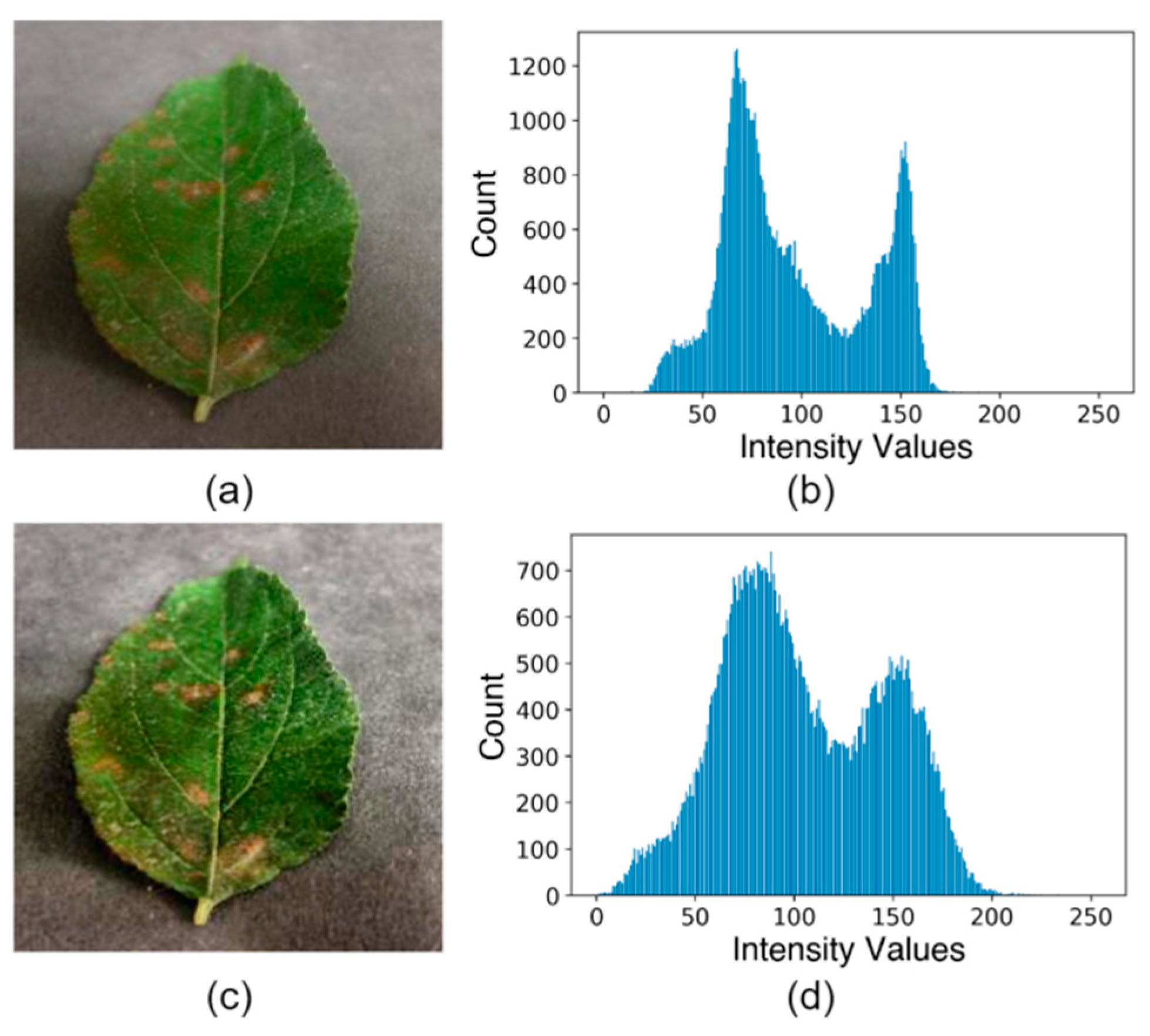
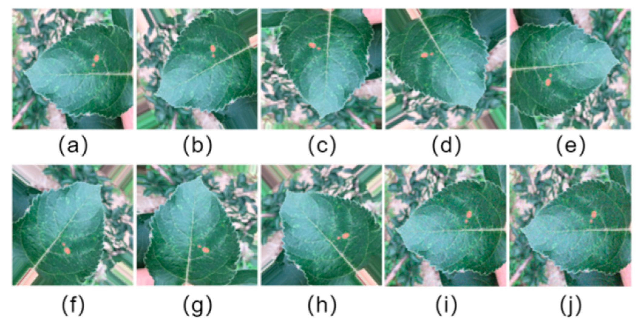
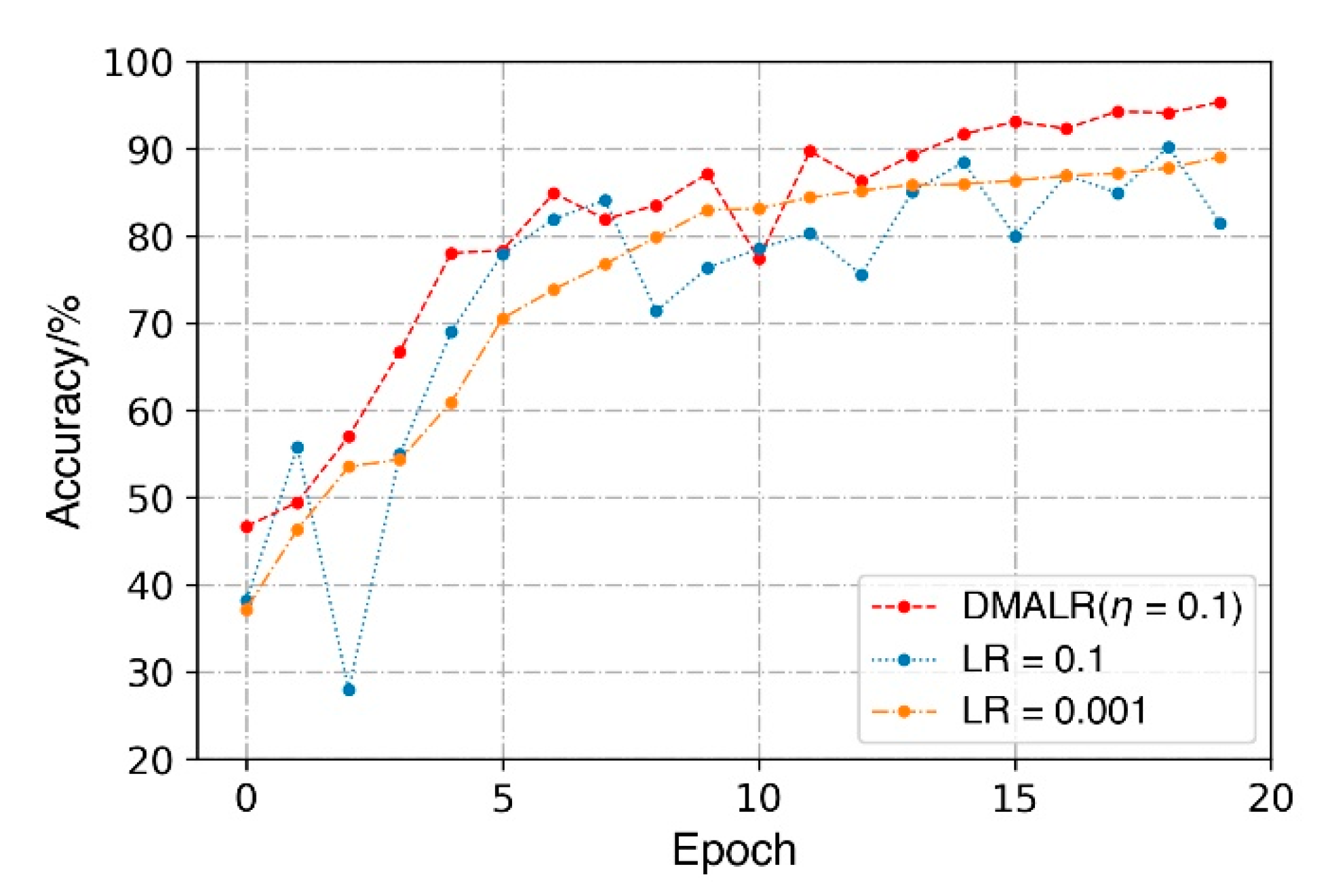
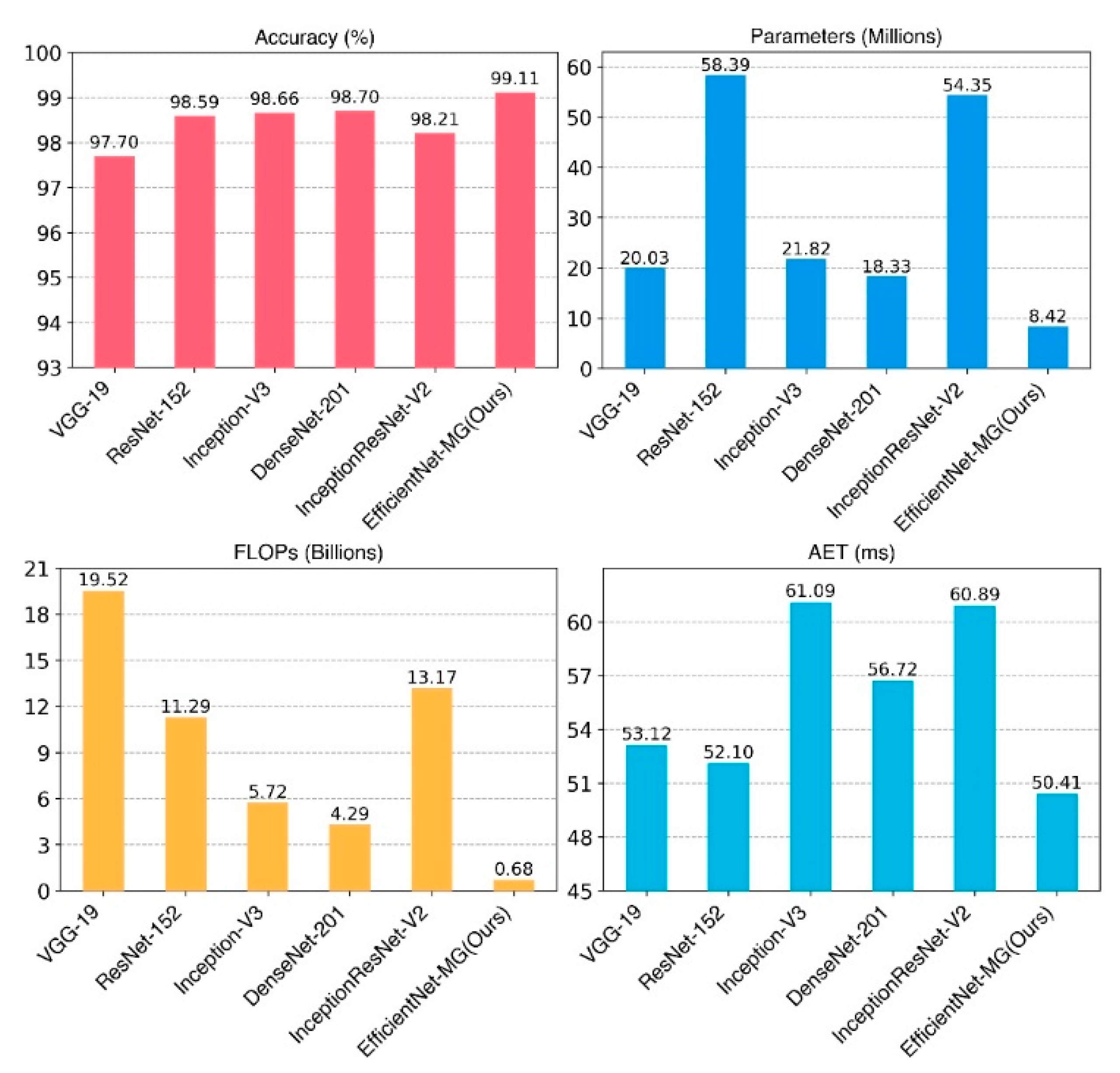
In this paper, to identify more categories of ALDs in the wild environment, a comprehensive dataset called AppleLeaf9 was constructed and opened. This dataset includes healthy apple leaves and eight types of ALDs in the field environment without limiting the shooting angles, noise, and other factors. AppleLeaf9 will help agricultural practitioners better apply CNN models to solve more practical problems on ALDs. CLAHE and some data augmentation methods were used for dataset preprocessing. Then, an accurate and lightweight CNN model, namely EfficientNet-MG, was proposed for ALD identification. Moreover, DMALR was proposed to advance the training effect of the CNN models. The experimental results showed that EfficientNet-MG achieves an accuracy of 99.11% with only 8.42 M parameters and 0.68 B FLOPs for healthy apple leaves and eight types of ALDs. In addition, EfficientNet-MG can identify an ALD image in the wild environment with only 50.41 ms. In the metrics of accuracy, parameters, FLOPs, and AET, EfficientNet-MG outperformed the five classical CNN models. Therefore, EfficientNet-MG is an accurate, lightweight, and robust CNN model for ALD identification in terms of overall performance, which provides an effective method for improving the yield and quality of apples. There is still a shortcoming in this paper: ALDs were not classified and diagnosed according to their degree of disease. In future work, more research can be improved in the following aspects: (1) To provide more detailed disease indicators, we plan to assess the disease severity of ALDs based on the diseased area. (2) We plan to deploy the proposed EfficientNet-MG to mobile devices, such as mobile phones and UAVs.

References

1. Liu, B.; Fan, K.; Su, W.; Peng, Y. Two-Stage Convolutional Neural Networks for Diagnosing the Severity of Alternaria Leaf Blotch Disease of the Apple Tree. Remote Sens. 2022, 14, 2519. [Google Scholar] [CrossRef]
2. Praba, R.D.; Vennila, R.; Rohini, G.; Mithila, S.; Kavitha, K. Foliar Disease Classification in Apple Trees. In Proceedings of the 2021 International Conference on Advancements in Electrical, Electronics, Communication, Computing and Automation (ICAECA), Virtual Conference, 8–9 October 2021; pp. 1–5. [Google Scholar] [CrossRef]
3. Alvarez-Mendoza, C.I.; Teodoro, A.; Quintana, J.; Tituana, K. Estimation of Nitrogen in the Soil of Balsa Trees in Ecuador Using Unmanned Aerial Vehicles. In Proceedings of the IGARSS 2020—2020 IEEE International Geoscience and Remote Sensing Symposium, Waikoloa, HI, USA, 26 September–2 October 2020; pp. 4610–4613. [Google Scholar] [CrossRef]
4. Selvaraj, M.G.; Vergara, A.; Ruiz, H.; Safari, N.; Elayabalan, S.; Ocimati, W.; Blomme, G. AI-powered banana diseases and pest detection. Plant Methods 2019, 15, 92. [Google Scholar] [CrossRef] [Green Version]
5. Yuan, L.; Huang, Y.; Loraamm, R.W.; Nie, C.; Wang, J.; Zhang, J. Spectral analysis of winter wheat leaves for detection and differentiation of diseases and insects. Field Crop Res. 2014, 156, 199–207. [Google Scholar] [CrossRef] [Green Version]
6. Yin, C.; Zeng, T.; Zhang, H.; Fu, W.; Wang, L.; Yao, S. Maize Small Leaf Spot Classification Based on Improved Deep Convolutional Neural Networks with a Multi-Scale Attention Mechanism. Agronomy 2022, 12, 906. [Google Scholar] [CrossRef]
7. Chuanlei, Z.; Shanwen, Z.; Jucheng, Y.; Yancui, S.; Jia, C. Apple leaf disease identification using genetic algorithm and correlation based feature selection method. Int. J. Agr. Biol. Eng. 2017, 10, 74–83. [Google Scholar] [CrossRef]
8. Singh, S.; Gupta, S.; Tanta, A.; Gupta, R. Extraction of Multiple Diseases in Apple Leaf Using Machine Learning. Int. J. Image Graph. 2021, 21, 2140009. [Google Scholar] [CrossRef]
9. LeCun, Y.; Bengio, Y.; Hinton, G. Deep learning. Nature 2015, 521, 436–444. [Google Scholar] [CrossRef]
10. Huang, G.; Liu, Z.; van der Maaten, L.; Weinberger, K.Q. Densely Connected Convolutional Networks. In Proceedings of the 30th IEEE Conference on Computer Vision and Pattern Recognition (CVPR 2017), Honolulu, HI, USA, 21–26 July 2016; IEEE: New York, NY, USA, 2017; pp. 2261–2269. [Google Scholar] [CrossRef]
11. Zhong, Y.; Zhao, M. Research on deep learning in apple leaf disease recognition. Comput. Electron. Agr. 2020, 168, 105146. [Google Scholar] [CrossRef]
12. Yadav, D.; Yadav, A.K. A Novel Convolutional Neural Network Based Model for Recognition and Classification of Apple Leaf Diseases. Trait. Signal 2020, 37, 1093–1101. [Google Scholar] [CrossRef]
13. He, K.; Zhang, X.; Ren, S.; Sun, J. Deep residual learning for image recognition. In Proceedings of the IEEE Conference on Computer Vision and Pattern Recognition (CVPR), Las Vegas, NV, USA, 27–30 June 2016; pp. 770–778. [Google Scholar] [CrossRef] [Green Version]
14. Jiang, H.; Xue, Z.P.; Guo, Y. Research on Plant Leaf Disease Identification Based on Transfer Learning Algorithm. In Proceedings of the 4th International Conference on Artificial Intelligence, Automation and Control Technologies (AIACT 2020), Hangzhou, China, 24–26 April 2020; Volume 1576, p. 012023. [Google Scholar] [CrossRef]
15. Lin, M.; Chen, Q.; Yan, S. Network in Network. arXiv 2013, arXiv:1312.4400. [Google Scholar]
16. Chollet, F. Xception: Deep learning with depthwise separable convolutions. In Proceedings of the IEEE Conference on Computer Vision and Pattern Recognition, Honolulu, HI, USA, 21–26 July 2017; pp. 1251–1258. [Google Scholar] [CrossRef] [Green Version]
17. Chao, X.; Sun, G.; Zhao, H.; Li, M.; He, D. Identification of Apple Tree Leaf Diseases Based on Deep Learning Models. Symmetry 2020, 12, 1065. [Google Scholar] [CrossRef]
18. Howard, A.G.; Zhu, M.; Chen, B.; Kalenichenko, D.; Wang, W.; Weyand, T.; Andreetto, M.; Adam, H. Mobilenets: Efficient convolutional neural networks for mobile vision applications. arXiv 2017, arXiv:1704.04861. [Google Scholar] [CrossRef]
19. Bi, C.; Wang, J.; Duan, Y.; Fu, B.; Kang, J.; Shi, Y. MobileNet based apple leaf diseases identification. Mob. Networks Appl. 2020, 27, 172–180. [Google Scholar] [CrossRef]
20. Simonyan, K.; Zisserman, A. Very deep convolutional networks for large-scale image recognition. arXiv 2014, arXiv:1409.1556. [Google Scholar] [CrossRef]
21. Ioffe, S.; Szegedy, C. Batch normalization: Accelerating deep network training by reducing internal covariate shift. In Proceedings of the International Conference on Machine Learning, Lille, France, 6–11 July 2015; pp. 448–456. [Google Scholar]
22. Hughes, D.; Salathé, M. An open access repository of images on plant health to enable the development of mobile disease diagnostics. arXiv 2015, arXiv:1511.08060. [Google Scholar] [CrossRef]
23. Yan, Q.; Yang, B.; Wang, W.; Wang, B.; Chen, P.; Zhang, J. Apple leaf diseases recognition based on an improved convolutional neural network. Sensors 2020, 20, 3535. [Google Scholar] [CrossRef]
24. Luo, Y.; Sun, J.; Shen, J.; Wu, X.; Wang, L.; Zhu, W. Apple Leaf Disease Recognition and Sub-Class Categorization Based on Improved Multi-Scale Feature Fusion Network. IEEE Access 2021, 9, 95517–95527. [Google Scholar] [CrossRef]
25. Yu, H.; Cheng, X.; Chen, C.; Heidari, A.A.; Liu, J.; Cai, Z.; Chen, H. Apple leaf disease recognition method with improved residual network. Multimed. Tools Appl. 2022, 81, 7759–7782. [Google Scholar] [CrossRef]
26. Pradhan, P.; Kumar, B.; Mohan, S. Comparison of various deep convolutional neural network models to discriminate apple leaf diseases using transfer learning. J. Plant Dis. Prot. 2022, 129, 1461–1473. [Google Scholar] [CrossRef]
27. Gao, Y.; Wang, H.; Li, M.; Su, W. Automatic Tandem Dual BlendMask Networks for Severity Assessment of Wheat Fusarium Head Blight. Agriculture 2022, 12, 1493. [Google Scholar] [CrossRef]
28. Huang, Y.; Zhang, J.; Zhang, J.; Yuan, L.; Zhou, X.; Xu, X.; Yang, G. Forecasting Alternaria Leaf Spot in Apple with Spatial-Temporal Meteorological and Mobile Internet-Based Disease Survey Data. Agronomy 2022, 12, 679. [Google Scholar] [CrossRef]
29. Thapa, R.; Zhang, K.; Snavely, N.; Belongie, S.; Khan, A. The Plant Pathology Challenge 2020 data set to classify foliar disease of apples. Appl. Plant Sci. 2020, 8, e11390. [Google Scholar] [CrossRef] [PubMed]
30. Feng, J.F.J.; Chao, X.C.X. Apple Tree Leaf Disease Segmentation Dataset; Science Data Bank: Beijing, China, 2022. [Google Scholar] [CrossRef]
31. Pizer, S.M.; Amburn, E.P.; Austin, J.D.; Cromartie, R.; Geselowitz, A.; Greer, T.; ter Haar Romeny, B.; Zimmerman, J.B.; Zuiderveld, K. Adaptive histogram equalization and its variations. Comput. Vis. Graph. Image Process. 1987, 39, 355–368. [Google Scholar] [CrossRef]
32. Zuiderveld, K. Contrast limited adaptive histogram equalization. In Graphics Gems; Elsevier: Amsterdam, The Netherlands, 1994; pp. 474–485. [Google Scholar]
33. Garg, R.; Mittal, B.; Garg, S. Histogram equalization techniques for image enhancement. Int. J. Electron. Commun. Technol. 2011, 2, 107–111. [Google Scholar]
34. Zhang, P.; Yang, L.; Li, D. EfficientNet-B4-Ranger: A novel method for greenhouse cucumber disease recognition under natural complex environment. Comput. Electron. Agr. 2020, 176, 105652. [Google Scholar] [CrossRef]
35. Tan, M.; Chen, B.; Pang, R.; Vasudevan, V.; Sandler, M.; Howard, A.; Le, Q.V. Mnasnet: Platform-aware neural architecture search for mobile. In Proceedings of the IEEE/CVF Conference on Computer Vision and Pattern Recognition, Long Beach, CA, USA, 15–20 June 2019; pp. 2820–2828. [Google Scholar] [CrossRef] [Green Version]
36. Chowdhury, N.K.; Kabir, M.A.; Rahman, M.; Rezoana, N. ECOVNet: An Ensemble of Deep Convolutional Neural Networks Based on EfficientNet to Detect COVID-19 From Chest X-rays. arXiv 2020, arXiv:2009.11850. [Google Scholar] [CrossRef]
37. Sandler, M.; Howard, A.; Zhu, M.; Zhmoginov, A.; Chen, C. Mobilenetv2: Inverted residuals and linear bottlenecks. In Proceedings of the IEEE Conference on Computer Vision and Pattern Recognition, Salt Lake City, UT, USA, 18–23 June 2018; pp. 4510–4520. [Google Scholar] [CrossRef] [Green Version]
38. Hu, J.; Shen, L.; Sun, G. Squeeze-and-Excitation Networks. In Proceedings of the 31st IEEE/CVF Conference on Computer Vision and Pattern Recognition (CVPR), Salt Lake City, UT, USA, 18–23 June 2018; pp. 7132–7141. [Google Scholar] [CrossRef] [Green Version]
39. Fang, Z.; Ren, J.; MacLellan, C.; Li, H.; Zhao, H.; Hussain, A.; Fortino, G. A novel multi-stage residual feature fusion network for detection of COVID-19 in chest X-ray images. IEEE Trans. Mol. Biol. Multi-Scale Commun. 2021, 8, 17–27. [Google Scholar] [CrossRef] [PubMed]
40. Clevert, D.; Unterthiner, T.; Hochreiter, S. Fast and accurate deep network learning by exponential linear units (elus). arXiv 2015, arXiv:1511.07289. [Google Scholar] [CrossRef]
41. Yu, C.; Su, Z. Symmetrical Gaussian Error Linear Units (SGELUs). arXiv 2019, arXiv:1911.03925. [Google Scholar] [CrossRef]
42. Hendrycks, D.; Gimpel, K. Gaussian error linear units (gelus). arXiv 2016, arXiv:1606.08415. [Google Scholar] [CrossRef]
43. Xie, C.; Tan, M.; Gong, B.; Yuille, A.; Le, Q.V. Smooth adversarial training. arXiv 2020, arXiv:2006.14536. [Google Scholar] [CrossRef]
44. Pan, S.J.; Yang, Q. A survey on transfer learning. IEEE Trans. Knowl. Data Eng. 2009, 22, 1345–1359. [Google Scholar] [CrossRef]
45. Rahman, T.; Chowdhury, M.E.; Khandakar, A.; Islam, K.R.; Islam, K.F.; Mahbub, Z.B.; Kadir, M.A.; Kashem, S. Transfer learning with deep convolutional neural network (CNN) for pneumonia detection using chest X-ray. Appl. Sci. 2020, 10, 3233. [Google Scholar] [CrossRef]
46. Bottou, L. Large-scale machine learning with stochastic gradient descent. In Proceedings of the COMPSTAT’2010, Paris, France, 22–27 August 2010; pp. 177–186. [Google Scholar]
47. Szegedy, C.; Vanhoucke, V.; Shlens, J. Rethinking the Inception Architecture for Computer Vision. In Proceedings of the Computer Vision Fundation, Columbus, OH, USA, 23–28 June 2014; pp. 2818–2826. [Google Scholar] [CrossRef]
48. Szegedy, C.; Ioffe, S.; Vanhoucke, V.; Alemi, A.A. Inception-v4, inception-ResNet and the impact of residual connections on learning. In Proceedings of the Thirty-First AAAI Conference on Artificial Intelligence, San Francisco, CA, USA, 4–9 February 2017. [Google Scholar]
Figure 1. Distribution of image sources in AppleLeaf9.
Agronomy 12 02784 g001
Figure 2. Samples of AppleLeaf9: (a) healthy; (b) Alternaria leaf spot; (c) brown spot; (d) frogeye leaf spot; (e) grey spot; (f) mosaic; (g) powdery mildew; (h) rust; (i) scab.
Agronomy 12 02784 g002
Figure 3. Comparison between the original image and the CLAHE image: (a) original image; (b) histogram of the greyscale image in (a); (c) result of enhancement using CLAHE; (d) histogram of the greyscale image in (c).
Agronomy 12 02784 g003
Figure 4. Examples of dataset augmentation: (a) original image; (b) rotated 45°; (c) rotated 90°; (d) rotated 135°; (e) rotated 180°; (f) rotated 225°; (g) rotated 270°; (h) rotated 315°; (i) salt-and-pepper noise; (j) Gaussian noise.
Agronomy 12 02784 g004
Figure 5. Structure of MBConv block.
Agronomy 12 02784 g005
Figure 6. Proposed EfficientNet-MG for ALD identification.
Agronomy 12 02784 g006
Figure 7. Transfer learning process.
Agronomy 12 02784 g007
Figure 8. Block diagram of the experimental procedure.
Agronomy 12 02784 g008
Figure 9. Comparison of training effects in fold 1.
Agronomy 12 02784 g009
Figure 10. Convergence comparison: (a) loss; (b) accuracy.
Agronomy 12 02784 g010
Figure 11. Confusion matrix: (a) unnormalized; (b) normalized.
Agronomy 12 02784 g011
Figure 12. ROC curves of different categories.
Agronomy 12 02784 g012
Figure 13. Convergence comparison of different CNN models.
Agronomy 12 02784 g013
Figure 14. Performance of different models.
Agronomy 12 02784 g014
Figure 15. EfficientNet-MG and EfficientNet-B1 identification results with feature visualization: (a) original image; (b) L1; (c) L2; (d) L3; (e) L4; (f) identification results.
Agronomy 12 02784 g015