Simulation of Multi-Species Plant Communities in Perturbed and Nutrient-Limited Grasslands: Development of the Growth Model ModVege

Abstract

Simulating the dynamics of plant species or types in grassland communities remains an open area of research for which the Community Simulation Model (CoSMo) offers novel approaches. The grassland model ModVege was first parameterised based on a functional vegetation typology, in which types “A” and “B” include fast-growing grass species with a phenology-dependent nutrient-capture strategy inherent to fertile grasslands, while the nutrient conservation strategy and late flowering characterise the other types as “b”. ModVege was then coupled to the CoSMo rule set to dynamically simulate the relative abundance of plant functional types or individual species, assessed across fertilised and unfertilised, abandoned and mown conditions in a grassland site of the Massif Central of France. While for the simulation of aboveground biomass, model performance is not unambiguously linked to explicit consideration of plant diversity, the simulation of relative abundance for the whole community is satisfactory (relative root mean square error of ~13–25% when simulating functional types and ~28–52% when simulating species). This study extends previous studies by coupling CoSMo, for the first time, to a grassland-specific model and applying it to conditions (long-term observations, extended number of plant species, absence of fertilisation, frequent mowing and abandonment) never investigated before.

1. Introduction

1.1. Plant Diversity in Grasslands

Grasslands often contain a high diversity of plants, which is of interest for wildlife conservation, for a diverse forage resource in relation to feed quality, and for the resources provided to micro- and macro-fauna [1,2]. This plant diversity can be described and studied using different approaches [3]. For instance, the number of individual species present in a grassland (species richness) informs on the ecological or patrimonial status of the communities. However, despite experimental evidence of causal relationships between species number, ecosystem productivity and carbon sequestration [4,5], species richness is not an accurate indicator of the agronomic value of grasslands (e.g., productivity, quality, precocity). For that, herbaceous species are often classified into three taxonomic groups, namely grasses, legumes and forbs, the latter two playing a decisive role in the overgrowth of mixtures [6]. Both species richness and taxonomic diversity do not take into account whether plant species or groups of species are similar or different in their attributes (or traits) [7]. Functional diversity highlights the traits of plant species to identify the main types of plant species present in a grassland based on biological characteristics (functional traits) that correspond to similar functioning or strategies [8]. In fact, plant functional traits mediated by plant species composition affect most key ecosystem properties, depending on the relative contribution of a given species to the total vegetation biomass [9,10,11]. As such, functional diversity characterises the agronomic value of grasslands, e.g., a grassland with high functional diversity can be exploited for its resilience to extreme weather events [12], and functional diversity can be an indicator of grassland ecosystem services [13,14].

1.2. Functional Typology

The concept of functional traits (or plant functional diversity), which provides a generic approach to characterise vegetation types [15], is attractive as a tool for inferring ecosystem processes (e.g., plant growth) through aggregated traits of dominant species other than weather, soil and management factors [14]. Plant traits and trait-based plant classifications thus provide a sound scientific basis for reckoning the provision of ecosystem services and guiding grassland management [16,17]. This can be done through a typology, i.e., a set of rules to define the characteristics of an observed system (here the kind of grassland), which facilitates its classification and the assessment of the ecosystem services provided [18]. Cruz et al. [19] conceived a grass species typology with the aim to provide support to grassland advisors via a generic method facilitating the manipulation of complex information, namely on the linkage between biodiversity and grassland performance (e.g., forage production). For that, Cruz et al. [19] and Theau et al. [20] proposed a classification of perennial forage grasses based on six functional characteristics to discriminate between biomass production and fodder quality of species mixtures. This functional typology was based on 38 grass species commonly found in the upland areas of central and southern France, which were characterised under similar and controlled pedo-climatic conditions in order to obtain differences only due to their physiological/morphological peculiarities. These peculiarities include the growth strategies (capture or conservation of resources) and phenology (early- or late-growth and flowering) of the plants, which are rendered from six morphological and phenological traits [21]: leaf dry matter content, specific leaf area, leaf lifespan, leaf resistance to breakage and, for the whole plant, flowering date and maximum plant height. This functional composition, based on the identification of dominant grass species and four main types (A, B, C, D) makes it possible to create a classification according to the dates of growth peaks, and the digestibility of leaves and stems. Types A and B (fast-growing, phenology-dependent nutrient-capture strategy) dominate in fertile grasslands, while the opposite is observed for types C and D (slow-growing, nutrient conservation strategy, late flowering). A-type and B-type grasslands are characterised by a high nutritive value in terms of digestibility for livestock feed at the beginning of the first vegetation cycle (and a rapid decline in nutritive value with early-maturity plants) and a high biomass accumulation [22]. Conversely, types C and D species are generally characterised by low digestibility values at the beginning of the cycle (followed by a slower decline during the rest of the vegetation cycle), due to later plant maturity and lower biomass accumulation [23]. Cruz et al. [24] defined additional types to characterise tall, late-flowering species in fertile (type “b”) or poor (type “d”) soils. From this knowledge-based classification, it is possible to parameterise alternative grassland types for modelling purposes [25,26].

1.3. Grassland Modelling

Simulation models combining community traits with soil, climate and management are widely used to predict grassland productivity and biophysical/biogeochemical cycles [27,28]. In these models, plant traits are generally considered as static inputs (i.e., model parameters) that characterise the mean vegetation of the community, which become specific and dynamic when plant diversity is taken into account. Modelling solutions linking the processes and dynamics of plant types to the processes and dynamics of communities are mostly integrated into specific models and for a limited number of species in a community [29,30,31,32]. High detail of plant interactions can be achieved at the expense of detailed process descriptions, while niche differentiation needs to be improved to simulate the coexistence of several species [33]. DynaGraM [34] addresses theoretical questions about the response of a grassland species model to climatic, edaphic and management-forcing agents as a function of the state of the plant community. Conceived as a model of resource competition [35], it represents the regulation of green biomass and plant competition from the standpoint of resource dynamics [36], integrating eco-physiological and biophysical details inherited from ModVege [25,26], originally developed to predict vegetation growth from permanent grasslands in central France. Another approach, the Community Simulation Model (CoSMo), provides a means for incorporating plant diversity in grassland models [37]. With a set of parameter values for each plant type in a community (individual species or groups of species such as functional types), CoSMo updates the relative abundance of different plant categories (at the level of individual species or taxonomic or functional groups of species) at each time step. The characterisation of the different plant types is performed using different sets of values for the same parameters (a common set of parameters for all plant categories). CoSMo translates environmental changes and farming practices into a numerical framework. Competition and changes in the relative abundance of plant categories are simulated in response to hierarchical environmental drivers (biophysical and management factors, triggered or continuous), which represent the suitability [38] of different plant categories to the conditions explored at each time step. On this basis, CoSMo derives (daily) vegetation parameter values for the plant community from the relative abundance of the different plant species or groups and the parameter values initially set to characterise the same plant species or group. These dynamically derived vegetation parameters are then used at each time step by the growth simulator (ModVege in our case). In doing so, CoSMo goes beyond the conventional assumption that the values assigned to the model parameters (by calibration, experimental measurement or from the literature) are time-invariant and remain constant throughout the simulation period, a simplification that may be too limiting to meet the challenges faced by agricultural systems, for which modelling cannot ignore plant diversity aspects [39]. Designed as a re-usable component, CoSMo was already coupled with generic crop models (CropSyst [40], WOFOST [41]) to explicitly and dynamically simulate the relative abundance of plant species in grasslands, and satisfactorily applied to annually mown grasslands in central Italy [42].

Starting from the need to extend and evaluate the potential of CoSMo to complex situations, the novelty of the present study lies in the use of a model specifically developed for the simulation of grasslands (ModVege), coupled with CoSMo. The objective was to assess it at a set of management conditions, observation periods and plant species/functional types, never before studied. A first approach, consistent with the level of complexity of the generic grassland simulator, dynamically models the relative abundance of functional types in a grassland community. A second approach adds complexity to ModVege to represent the dynamics of individual plant species in the community. The assessment of three modelling solutions—a grassland model in standalone, coupled versions for functional groups and individual species—was thus carried out for aboveground biomass and relative abundance of plant groups/species using multi-year field data from mown (fertilised or not) and undisturbed (abandoned) multispecies grasslands in the Massif Central of France.

2. Materials and Methods

2.1. The Modelling Framework

2.1.1. Generic Grassland Model (ModVege)

ModVege is a relatively simple process-based model that estimates herbage quantity and quality in managed, multi-species grasslands. It implements the conceptual framework originally proposed by [43,44] to calculate the mass flow in four structural compartments of aboveground biomass on a daily time-step (Supplementary Material, Figure S1). The model development is based on the assumption that community behaviour can be explained by the mean traits of dominant grasses. The model addresses six basic functional groups of grasses [45] that can be combined in different proportions to simulate a wide range of grassland communities [25]. Environmental constraints are associated with water scarcity, high radiation levels and temperature extremes, within a purely source-driven model, where potential growth is expressed as a function of the photosynthetic active radiation intercepted [46]. The processes contributing to biomass turnover are growth, senescence and abscission. The onset of growth is assumed to occur when the cumulative thermal time since 1 January exceeds 200 °C-d for the first time. Water availability is related to the fractional water content, W = WR/WHC, where WR is the current water reserve and WHC is the water holding capacity. A simple bucket approach is used to evaluate WR, where precipitation is considered as an input and actual evapotranspiration (AET) and drainage as outputs. Drainage is assumed to occur whenever the difference between precipitation and AET exceeds the soil’s absorption capacity, given by the difference between WHC and WR. Herbage growth is further controlled by the overall nutrient availability through a nutrient index, i.e., a relative measure of the overall nutritional status of the canopy, which can range from 0.35 in nutrient deficiency to 1.20 in heavily fertilised systems [47]. As there is no model component that simulates the nitrogen (N) cycle dynamically, the nutrition index is considered a site-specific parameter that can be reduced over time to represent the progressive depletion of N availability in unfertilised fields. Despite its simplifications, ModVege has been shown to perform well in a variety of environmental contexts and management regimes [48,49] and is being developed [50] for application as a decision-support system [51].

2.1.2. Community Simulation Model (CoSMo)

CoSMo simulates plant communities through a mean parameterisation based on the relative abundance of each group/species. Its approach can be coupled with any generic grassland simulator. The relative abundance of plant species (or groups of species) depends on the hierarchical aggregation of several drivers (each one assuming values between 0 and 1), which are estimated to characterise the suitability and competitiveness of each group/species in a given context. The generic simulator community parameterisation (y_community) is updated at a daily time-step, for each simulator parameter (y) based on the relative abundance (SCP) of each group/species (i) of n simulated groups/species in a mixed cover, as follows:

$$y_{community}={\forall }_y{\sum }_{i=1}^n\left(y_i·SC{P}_i\right)$$

(1)

where the universal quantifier is encoded as ∀ (“for all”).

SCP_i is derived at each time step (dt), dSCP_i(t), as follows:

$$\frac{dSC{P}_i\left(t\right)}{dt}=\left(\frac{Sf{s}_i\left(t\right)-\overline{SfS\left(t\right)}}{I}\right)$$

(2)

where Sf_Si(t) is the suitability factor for group/species i, Sf_S(t) is the mean suitability factor for all groups/species and 80 ≤ I ≤ 120 is an inertial replacement coefficient (suggested to be set at 100).

The term Sfs_i(t) is calculated from the hierarchical suitability function of driver q for the species i, HSf_i.q(t):

$$Sf{s}_i\left(t\right)={\sum }_{q=1}^z\left(HS{f}_{i,q}\left(t\right)\right)$$

(3)

where z is the number of drivers. In the current version, six drivers are hierarchically arranged: 1, management (cutting/grazing); 2, phenology; 3, air temperature; 4, light interception; 5, water availability; 6, N availability. They are hierarchically arranged as follows:

$$HS{f}_{i,q}\left(t\right)=\left\{\begin{array}{cc}S{f}_{i,q}\left(t\right)& q=1\\ \sqrt{HS{f}_{i,q-1}\left(t\right)}·S{f}_{i,q}\left(t\right)& \mathrm{otherwise}\end{array}\right.$$

(4)

Applying Equation (3) to the case of z=6, the result is:

$$\begin{array}{c}HS{f}_{i,1}\left(t\right)=S{f}_{i,1}\left(t\right)\\ HS{f}_{i,2}\left(t\right)=\sqrt{S{f}_{i,1}\left(t\right)}·S{f}_{i,2}\left(t\right)\\ HS{f}_{i,3}\left(t\right)=\sqrt[4]{S{f}_{i,1}\left(t\right)}·\sqrt{S{f}_{i,2}\left(t\right)}·S{f}_{i,3}\left(t\right)\\ HS{f}_{i,4}\left(t\right)=\sqrt[8]{S{f}_{i,1}\left(t\right)}·\sqrt[4]{S{f}_{i,2}\left(t\right)}·\sqrt{S{f}_{i,3}\left(t\right)}·S{f}_{i,4}\left(t\right)\\ HS{f}_{i,5}\left(t\right)=\sqrt[16]{S{f}_{i,1}\left(t\right)}·\sqrt[8]{S{f}_{i,2}\left(t\right)}·\sqrt[4]{S{f}_{i,3}\left(t\right)}·\sqrt{S{f}_{i,4}\left(t\right)}·S{f}_{i,5}\left(t\right)\\ HS{f}_{i,6}\left(t\right)=\sqrt[32]{S{f}_{i,1}\left(t\right)}·\sqrt[16]{S{f}_{i,2}\left(t\right)}·\sqrt[8]{S{f}_{i,3}\left(t\right)}·\sqrt[4]{S{f}_{i,4}\left(t\right)}·\sqrt{S{f}_{i,5}\left(t\right)}·S{f}_{i,6}\left(t\right)\end{array}$$

(5)

The methods for estimating the suitability functions of these drivers are described in Confalonieri [37] and Movedi et al. [42]. The application within ModVege required some adaptations of the CoSMo suitability functions to the features of the generic simulator. The ModVege-based implementation of the CoSMo suitability functions is described in the Supplementary Material (Section 2).

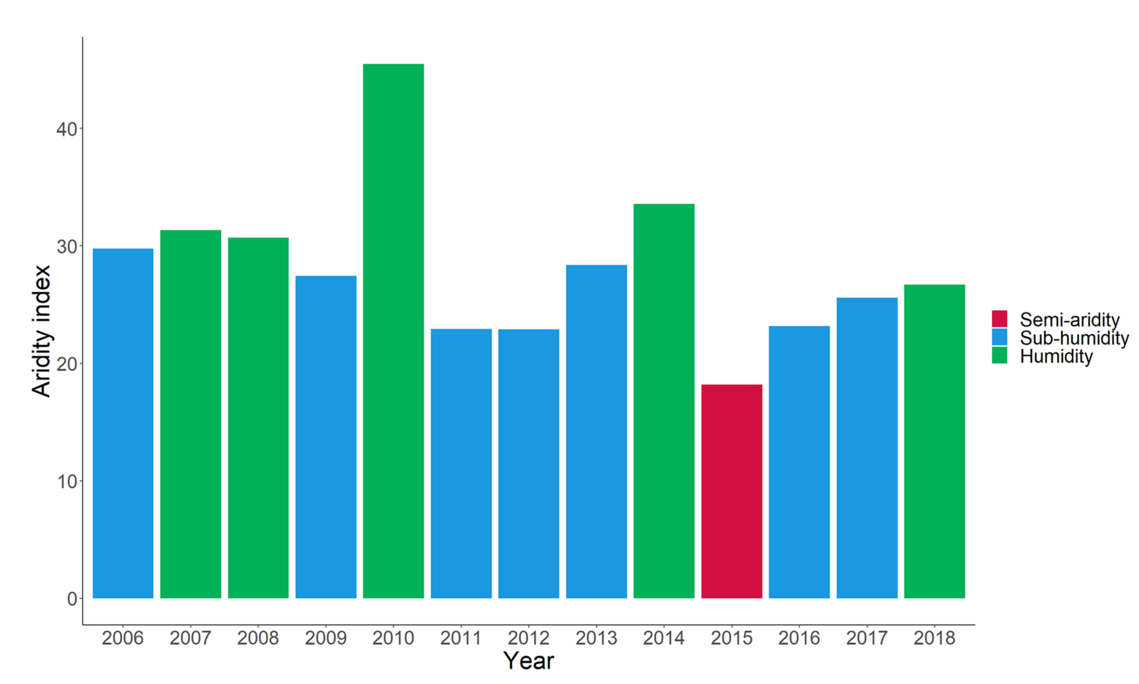
2.2. Study-Site and Experimental Design

We refer to the long-term observational system of Theix (45°43′ N, 03°01′ E, 880 m a.s.l.), located in the Massif Central of France (Supplementary Material, Figure S2). A designed experiment was established in 2005 on an area of ~3 ha, with the aim of analysing the response of permanent grasslands to changes in management practices [52] (Louault et al., 2017). The site is equipped with a meteorological station, which provides hourly values of global radiation, air temperature and precipitation, as well as soil temperature. The climate is semi-continental with a mean annual temperature of 8.7 °C and a mean yearly rainfall of 770 mm. It is essentially humid or sub-humid, according to the De Martonne-Gottmann aridity index [53], calculated annually as $b=\frac{1}{2}·\left[\frac{P_y}{T_y+10}+12·\left(\frac{p_a}{t_a+10}\right)\right]$, where P_y (mm) is the total annual precipitation, T_y (°C) is the mean annual temperature, p_a (mm) is the total precipitation of the driest month, T_a (°C) is the mean monthly temperature of the driest month. The index b offers the possibility of discriminating different thermo-pluviometric conditions during the study period (Figure 1), based on the ranges of values published by Diodato and Ceccarelli [54]: b < 5: extreme aridity; 5 ≤ b < 14: aridity; 15 ≤ b < 19: semi-aridity; 20 ≤ b < 29: sub-humidity; 30 ≤ b < 59: humidity; b ≥ 59: high humidity. The highest value of the aridity index (the lowest aridity), b = 46, was observed in 2010, a year with the highest rainfall (885 mm). Exceptionally, 2015 was a semi-arid year with below-average rainfall (585 mm) and the aridity index b = 18.

The soil developed from granitic bedrock and has different characteristics in the upper layer of the experimental site. The experimental design was thus repeated on two blocks or cambisol units, with block 1 being a eutric cambisol and block 2 being a colluvic material. Differences in soil characteristics (

Table 1. Soil properties of the grassland study-site (mean of the six plots per block).

Soil properties	Unit	Block 1		Block 2
Layer thickness	m	0.00–0.20	0.20–0.40	0.00–0.20	0.20–0.40
Clay	%	19.7	17.0	23.0	25.0
Silt	%	26.9	27.4	26.1	24.2
Sand	%	53.4	55.6	51.0	50.8
Carbon content	g kg−1	40.3	18.5	43.1	15.1
pH	-	5.9	6.2	6.0	6.5
Bulk density	g cm−3	0.94	1.23	0.89	1.18

) were also observed in terms of botanical composition. At the initial stage, the most abundant species with a cumulative frequency of ~80% were, in block 1, Cerastium glomeratum, Elymus repens, Festuca arundinacea, Lolium perenne, Poa pratensis, Taraxacum officinale, i.e., six species, and in block 2, Agrostis capillaris, Alopecurus pratensis, Holcus lanatus, Lolium perenne, Poa pratensis, Taraxacum officinale, Trifolium repens, Trisetum flavescens, i.e., eight species.

Management prior to 2003 consisted of a mixed regime with one to two cuts for silage or hay, with applications of mineral and organic fertilisers, followed by grazing in autumn. In the two years prior to the implementation of the experiment (2003–2004), three annual cuts were applied without fertilisation. Since 2005, treatments were applied, distinguishing between i) the level of herbage utilisation by rotational grazing of cattle without fertilisation (i.e., disturbance gradient; three treatments), and ii) the level of fertilisation under a fixed mowing regime (i.e., nutrient availability gradient; three treatments). Each treatment was repeated twice in each block, resulting in 28 plots. Cattle grazing treatments (not used in this study) were applied on 2200 m² plots while smaller plots (350–400 m²) were either abandoned (Ab) or used for fertilisation treatments. The fertiliser application was split in early spring, after the first and after the second mowing. Fertilisation treatments were: (1) NPK: annual addition of mineral nitrogen, phosphorus and potassium (on average 264 kg N ha⁻¹, 33 kg P ha⁻¹ and 189 kg K ha⁻¹); (2) PK: annual addition of mineral phosphorus and potassium (on average 26 kg P ha⁻¹ and 143 kg K ha⁻¹); (3) Null: no fertilisation. More details are in Louault et al. [52]. For the modelling, the data corresponding to the NPK, Null and Ab treatments were used as a block mean. In order to highlight the properties and potential of the modelling solutions, we opted for a comparison of the most contrasting treatments (fully fertilised and unfertilised), so the PK treatment was not used for model assessment at this stage.

2.3. Experimental Data

Aboveground standing biomass and relative abundance of plant species were determined experimentally in mown and unmown plots. Biomass was harvested from the unmown (i.e., abandoned) plots for research purposes. Aboveground biomass (AGB hereafter) was determined in four sampling areas per plot (0.3 × 0.6 m² in the abandonment and 0.6 × 0.6 m² otherwise) at ~0.055 m height, harvested up to three times a year in May, July and October, after a cleaning cut at the end of winter. The sampling area was moved within the plot at each cutting date and the aboveground biomass was removed at the beginning of the regrowth period. Herbage samples were oven dried (60 °C, 48 h). For mown plots, annual herbage production was calculated as the sum of the three sampling dates (May, July, October, first, second and third cut, respectively).

The relative abundance of plant species in each treatment was determined from 2006 to 2018 (all years except 2009, when the botanical determination was not carried out in an observatory set-up phase during which annual survey designs were not yet in place), using 40 pinpoints regularly spaced along two to three fixed transects. The presence/absence of species was recorded at each of the 40 pinpoints. The relative abundance of each species was calculated at the plot level [55], normalised to the sum of the presence of all species and expressed as a percentage.

The total number of plant species recorded at least once in blocks 1 and 2 during the study period of ~50 in the Null treatment, compared to ~35–40 with full fertilisation or abandonment (Supplementary Material, Table S1), reflects the positive effect of cutting and no N input on species richness [56]. In this study (and in agreement with Movedi et al. [42]), we based the modelling work on the relative abundances of dominant species or functional groups. In order to limit the uncertainties related to the initialisation and parameterisation of minor groups/species, a practical threshold of 0.04 (4%) of the mean relative abundance during the simulated period was set, in order to exclude groups/species present with an abundance lower than this threshold. For modelling purposes, the relative abundances of the dominant types/species were then recalculated by relating the relative abundance of each species (

Table 2. Relative abundances of dominant species (two blocks and three treatments). Mean values observed over the study period (Obs) were recalculated (Rec) with respect to the dominant species. Here, P. pratensis could include a few specimens identified as Poa angustifolia, due to ambiguous determination.

NPK			Null			Ab
Species	Relative Abundances		Species	Relative Abundances		Species	Relative Abundances
	Obs	Rec		Obs	Rec		Obs	Rec
Block 1
Elymus repens	0.26	0.31	Achillea millefolium	0.04	0.06	Alopecurus pratensis	0.13	0.17
Festuca arundinacea	0.09	0.11	Elymus repens	0.05	0.07	Arrhenatherum elatius	0.04	0.05
Lolium multiflorum	0.07	0.09	Festuca arundinacea	0.09	0.13	Dactylis glomerata	0.04	0.05
Poa pratensis	0.15	0.17	Holcus lanatus	0.05	0.07	Elymus repens	0.27	0.35
Stellaria media	0.04	0.05	Poa pratensis	0.12	0.17	Festuca arundinacea	0.06	0.07
Taraxacum officinale	0.21	0.25	Poa trivialis	0.05	0.08	Galium aparine	0.04	0.05
			Taraxacum officinale	0.16	0.22	Poa pratensis	0.16	0.20
			Trifolium repens	0.14	0.29	Urtica dioica	0.04	0.05
Sum	0.82	1.00	Sum	0.70	1.00	Sum	0.78	1.00
Nb. of species	6		Nb. of species	8		Nb. of species	8
Block 2
Achillea millefolium	0.06	0.07	Achillea millefolium	0.04	0.07	Alopecurus pratensis	0.30	0.46
Alopecurus pratensis	0.18	0.23	Alopecurus pratensis	0.08	0.11	Arrhenatherum elatius	0.06	0.08
Holcus lanatus	0.07	0.08	Festuca arundinacea	0.05	0.07	Elymus repens	0.04	0.07
Lolium perenne	0.06	0.07	Lolium perenne	0.09	0.13	Holcus lanatus	0.04	0.07
Poa pratensis	0.17	0.20	Poa pratensis	0.12	0.18	Poa pratensis	0.11	0.18
Stellaria media	0.04	0.05	Taraxacum officinale	0.13	0.18	Urtica dioica	0.09	0.14
Taraxacum officinale	0.15	0.19	Trifolium repens	0.11	0.15
Trisetum flavescens	0.08	0.10	Trisetum flavescens	0.08	0.12
Sum	0.80	1.00	Sum	0.70	1.00	Sum	0.72	1.00
Nb. of species	8		Nb. of species	8		Nb. of species	6

) or functional types (

Table 3. Relative abundances of functional groups (grass species in two blocks and three treatments). Mean values observed over the study period (Obs) were recalculated (Rec) with respect to the dominant groups.

	NPK		Null		Ab
Functional Group	Relative Abundances		Relative Abundances		Relative Abundances
	Obs	Rec	Obs	Rec	Obs	Rec
Block 1
A	0.07	0.07	0.21	0.21	0.24	0.24
B	0.45	0.45	0.49	0.49	0.34	0.34
b	0.48	0.48	0.30	0.30	0.42	0.42
Sum	1.00	1.00	1.00	1.00	1.00	1.00
Block 2
A	0.47	0.47	0.39	0.40	0.59	0.61
B	0.33	0.33	0.32	0.32	0.27	0.28
b	0.20	0.20	0.28	0.28	0.11	0.11
Sum	1.00	1.00	0.99	1.00	0.97	1.00

) to the sum of the abundances. For instance, L. perenne was excluded from the list of dominant species in the block 1 treatments, with 2.0% (NPK) and 2.8% (Null), and in the block 2 abandonment, with 0.3%. On the other hand, it was included in the simulated species of the NPK and Null treatments in block 2, where its relative abundance is ~9%. Similarly, H. lanatus was excluded from the NPK treatment in block 1, where it is present at ~1%, while its presence amounts to ~8% in the same treatment in block 2, and is below the critical threshold in all other treatments except the Ab treatment in block 2, where it is at the 4% abundance threshold. We also underline that, when present, S. media is at the 4% abundance threshold in the fertilised treatment of both blocks. It can also be seen that P. pratensis is the only species present in all situations, while occasional forbs such as G. aparine (block 1) and U. dioica (both blocks) are only present in the abandoned plots (about 4–7% on average and mostly absent in the first years; Table S4 in Supplementary Material). One only legume species, T. repens, is present above the 4% threshold (10–11%) in both the unfertilised mown treatments. The selected species have a total abundance of ≥70%, and even ≥80% in the NPK treatments (Table 2).

In terms of functional grass typologies, type C was only marginally present in the unfertilised and abandoned treatments of block 2 (or absent for the rest), where the dominating groups A, B and b covered nearly 100% of abundances (Table 3).

Biomass yield and abundance data for plant types and species used for the modelling work are summarised in Tables S2–S4 of Supplementary Material.

2.4. Simulation Design and Model Evaluation

Simulations were designed and model evaluation was carried out to determine whether (i) CoSMo-based ModVege solutions simulated the relative abundance of plant (grass) functional types and species, and (ii) differences in simulated AGB were caused by the explicit simulation of plant diversity, by comparing the CoSMo-based and stand-alone ModVege solutions. Standalone (ModVege) and coupled (ModVege-CoSMo) modelling solutions were configured using daily weather data retrieved from the CLIMATIK database (through the INRAE portal, https://www6.paca.inrae.fr/agroclim/Les-outils, accessed on 7 October 2022) and management data as determined at the experimental site, and parameterised for each treatment of both blocks (Supplementary Material). In particular, simulations were performed with common sets of ModVege and CoSMo parameters (Tables S5 and S8) and type- and plant-specific parameters for either ModVege (Tables S6 and S7) or CoSMo (Tables S9 and S10). Some ModVege parameters were extracted from published literature for (grass-based) functional types [25]. Otherwise, the datasets described in Section 2.3 were used for the calibration of model parameters. ModVege stand-alone was first run for each functional type separately (A, B and b) and then the daily community AGB was obtained as a weighted mean of the three functional types, using for each treatment the mean abundances of each type over the period 2006–2018 (Table 3) as a weighting factor. The calibration work was carried out through a trial-and-error process comparing the model estimates with observational data while ensuring biologically interpretable plant parameters by modifying their values within plausible ranges. For instance, the parameters ST1 = 800 °C-d and ST2 = 1200 °C-d of G. aparine (Table S7) were adapted from the ranges of values provided by Theau et al. [20], and a similar approach was adopted for the other species. For the functional types, the maximum leaf area index values (LAImax > 9 m² m⁻²; Table S9) were calibrated to the upper limit of the LAI of grasslands, which is rarely higher than 10 [57]. As well, as the canopy height varies by several folds, mainly from 0.25 to 1.50 m [58], the maximum plant height (MaxHeight) was calibrated below the upper limit of 2.0 m [59]. For specific leaf area (SLA), we used (Table S7) the values provided by Bourdôt [60] for A. millefolium (0.017 m² g⁻¹) and by Ianovici et al. [61] for T. officinale (0.048 m² g⁻¹), while the SLA value used for U. dioica (0.023 m² g⁻¹) is the one provided by Gulías et al. [62] for Urtica atrovirens, and for G. aparine and T. repens, 0.048 m² g⁻¹ and 0.018 m² g⁻¹ are within the ranges of values provided by Poorter and de Jong [63] and Nölke et al. [64], respectively. Theau et al. [20] also provided ranges of values for maximum plant heights (e.g., from <0.4 for T. officinale, S. media and T. repens to >0.9 m for G. aparine, A. millefolium and U. dioica) to which we have referred for the calibrated values attributed to this CoSMo parameter (Table S10). For each type/species, the first determined (and recalculated) relative abundance was used to initialise CoSMo at the start of the simulation (1 January 2006).

The agreement between simulated and observed values of AGB and relative abundance of plant types/species (the latter only for CoSMo-based modelling solutions) was evaluated according to five commonly used metrics (RRMSE, RMAE, R², R, CRM) of model performance [65]. The relative root mean square error (optimum, 0 ≤ RRMSE (%) < ∝) and the relative mean absolute error (optimum, 0 ≤ RMAE (%) < ∝) indicate how far the estimates are from the actual data: both explain this concept in relative terms (percentage over the mean), the former in square terms and the second in absolute terms. Squaring emphasises larger differences, a feature that results in giving more weight to large deviations. Algebraically, RMAE ≤ RRMSE (due to the influence of squaring larger values), with these metrics being approximately equal if the absolute differences are of similar magnitude. This suggests that the absolute differences are more robust (less sensitive) to large biases than squared differences. The coefficient of determination (0 ≤ R² ≤ 1, optimum) is the squared measure of the linear correlation coefficient (−1 ≤ R ≤ 1, optimum) between the estimates and the observations: it assesses the goodness-of-fit of the model, i.e., the proportion of the observed variance explained by the estimates. The coefficient of residual mass (CRM) is a measure of the tendency of the model to overestimate (CRM < 0) or underestimate (CRM > 0) the observations.

We also evaluated the mean values of grassland community traits as estimated on a daily basis with CoSMo-based solutions according to the relative abundance of species/types. In the absence of observations, the values of two canopy traits (maximum height and specific leaf area) were appreciated for their variation over time, compared to the constant values attributed to the corresponding parameters of the species/types composing the community.

3. Results

Results are presented via a set of performance metrics calculated separately by output, block and treatment for the whole simulation period (Supplementary Material). For AGB, we compared standalone ModVege and its CoSMo-based solutions (Table S11). The estimates of relative plant abundances obtained with the two CoSMo-based modelling solutions were evaluated for both functional types (Table S12) and species (Table S13), either taken individually or aggregated by taxonomic groups and for the whole community.

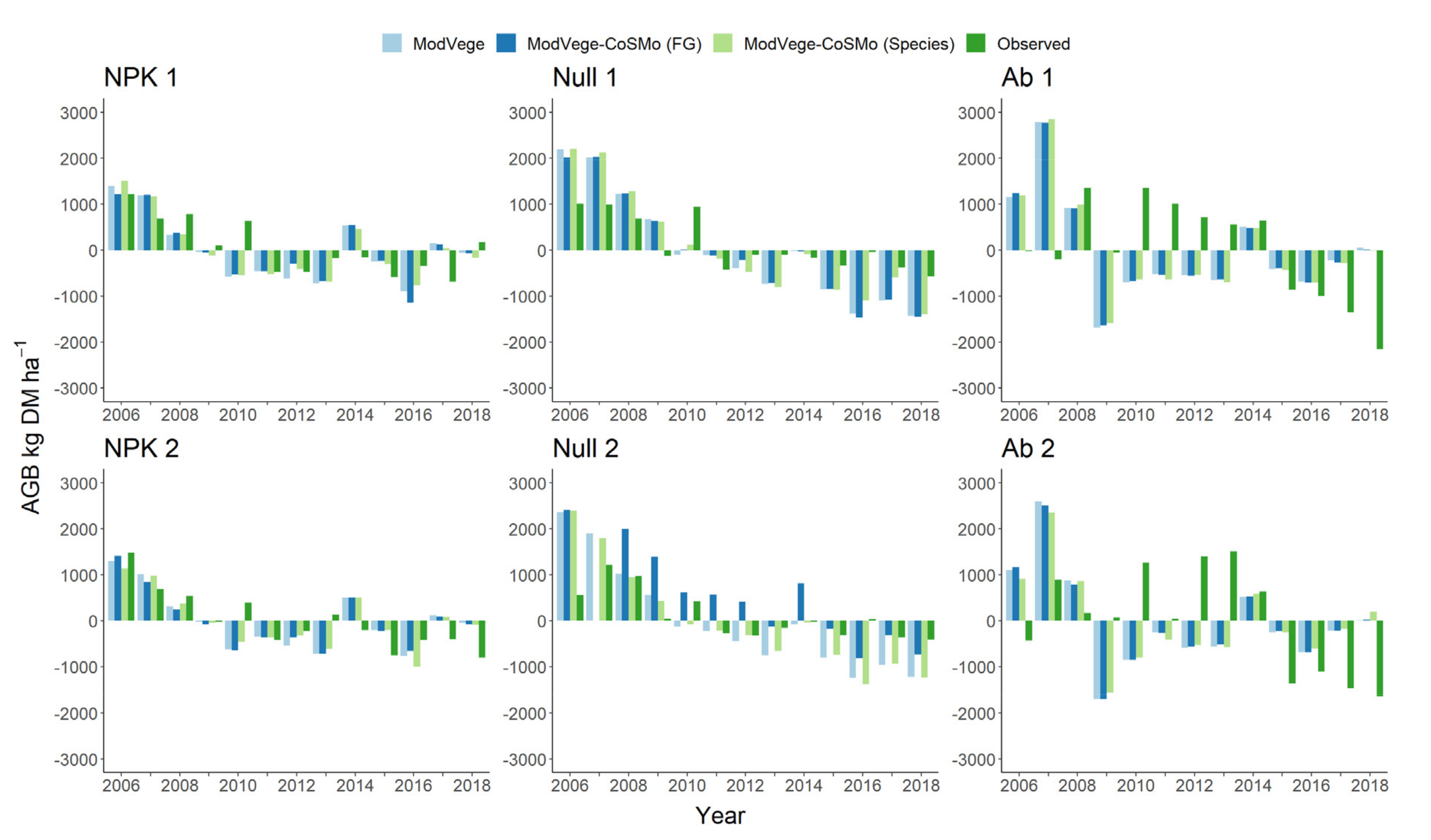
3.1. Evaluation of Modelling Solutions for Grassland Biomass Production

CoSMo-based and standalone modelling solutions performed similarly (Supplementary Material, Table S11) with <1.2 t ha⁻¹ AGB difference between simulations and observations on average (RRMSE~70%, RMAE~54% on average). In most cases, CRM values were negative, indicating a general model overestimation of the observed AGB (with the exception of CoSMo-based versions in the abandoned plots, with CRM from 0.07 to 0.12). The unfertilised (stressed and perturbed) plots were the most difficult to simulate (RRMSE > 100%). Although error amounts were lower for abandoned plots (RRMSE~40%, RMAE < 40%), with no substantial differences between modelling solutions, simulated and observed data were less correlated (R~0.4) under these stressed (unperturbed) conditions, reflected in a limited fit (R² ≤ 0.20) as data points do not line up around the 1:1 identity line (Figures S3–S5 in Supplementary Material). Overall, all three modelling solutions accounted for the decreasing trend in biomass production (annual anomalies) over the simulation period (Figure 2). In the NPK and Null treatments, R-values ranged from 0.60 (with ModVege-CoSMo for functional types under NPK 1) to 0.85 (with ModVege-CoSMo for the functional types under Null 2), while the quality of the simulations of the abandoned plots deteriorated towards the end of the simulation period. Some discrepancies between simulations and observations were also observed in the years 2008 to 2011, in the transition between mostly positive and mostly negative observed anomalies.

For the abandoned plots, the assessment at the summer sampling date (

Table 4. Evaluation of alternative modelling solutions for the simulation of aboveground biomass in the summer sampling of the abandoned plots (two blocks). Grey cells indicate the best performance. FG: functional groups.

Year	Doy	Observed Biomass	ModVege		ModVege-CoSMo FG		ModVege-CoSMo Species
			Simulated Biomass	Difference	Simulated Biomass	Difference	Simulated Biomass	Difference
		Block 1
2006	200	6742	6302	−440	5509	−1233	5503	−1239
2007	213	5781	8465	2684	7581	1800	7678	1897
2008	218	8116	7955	−161	7049	−1067	7072	−1044
2009	-	-	-	-	-	-	-	-
2010	201	7734	6372	−1362	5445	−2289	5592	−2142
2011	201	5674	4736	−938	3848	−1826	3675	−1999
2012	201	8560	6934	−1626	5992	−2568	6111	−2449
2013	198	6655	6495	−160	5587	−1068	5579	−1076
2014	203	6755	6357	−398	5447	−1308	5401	−1354
2015	202	4056	3591	−465	2890	−1166	2717	−1339
2016	202	4789	6955	2166	6026	1237	6051	1262
2017	205	4498	6332	1834	5376	878	5370	872
2018	204	3005	6744	3739	5822	2817	5758	2753
Mean		6030	6437	406	5548	−483	5542	−488
Minimum		3005	3591	−1626	2890	−2568	2717	−2449
Maximum		8560	8465	3739	7581	2817	7678	2753
		Block 2
2006	199	4576	6069	1493	5240	664	5124	548
2007	213	6822	8197	1375	7250	428	7285	463
2008	218	5832	7810	1978	6867	1035	6866	1034
2009	-	-	-	-	-	-	-	-
2010	201	8061	5982	−2079	5005	−3056	5135	−2926
2011	201	3867	5048	1181	4211	344	3945	78
2012	200	8227	6576	−1651	5664	−2563	5739	−2488
2013	198	7003	6395	−608	5494	−1509	5440	−1563
2014	203	6592	7859	1267	6948	152	5401	−1191
2015	202	3652	3911	259	3107	−545	2923	−729
2016	202	5131	6670	1539	5738	607	5786	655
2017	205	4312	6101	1789	5198	886	5169	857
2018	204	3656	6631	2975	5728	2072	5630	1974
Mean		5661	6437	776	5538	−124	5405	548
Minimum		3652	3911	−2079	3107	−3056	2910	−2926
Maximum		8227	8197	2975	7250	2072	6989	1974

) indicates that, on average, the three modelling solutions tended to converge with the observations: <1.0 t ha⁻¹ deviation down to ~0.1 t ha⁻¹ with the CoSMo-based functional group solution in block 2.

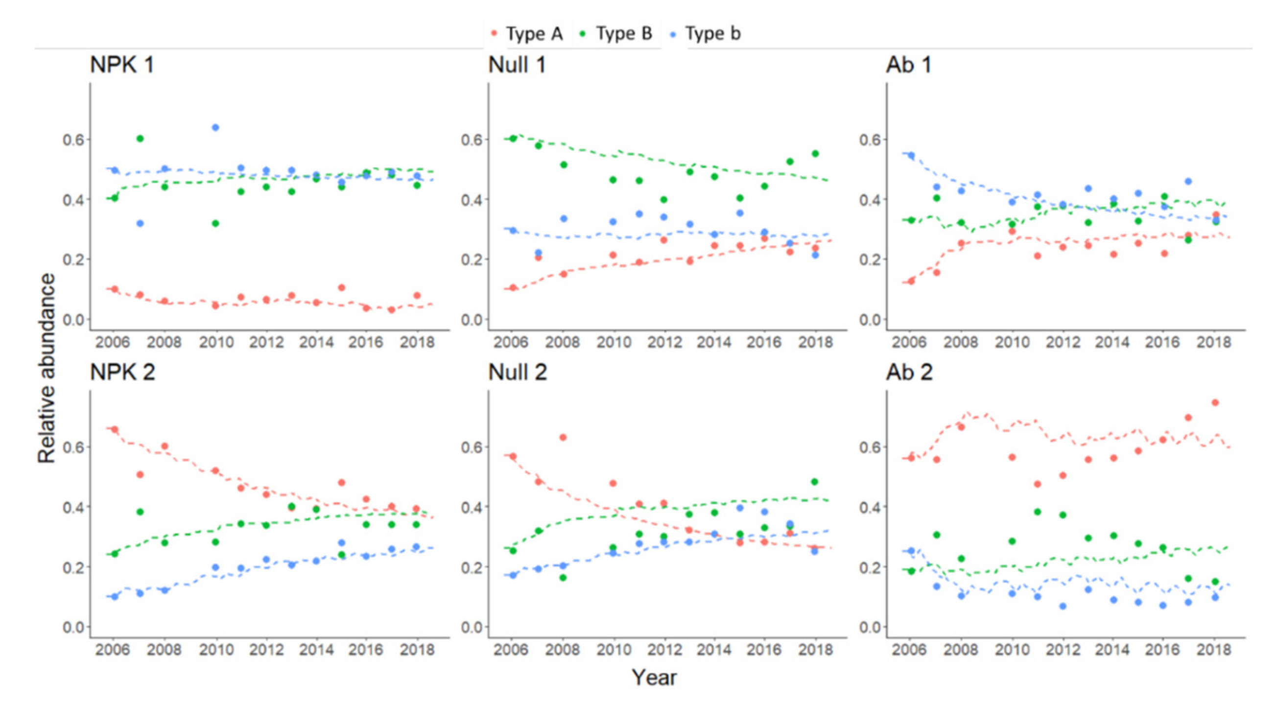
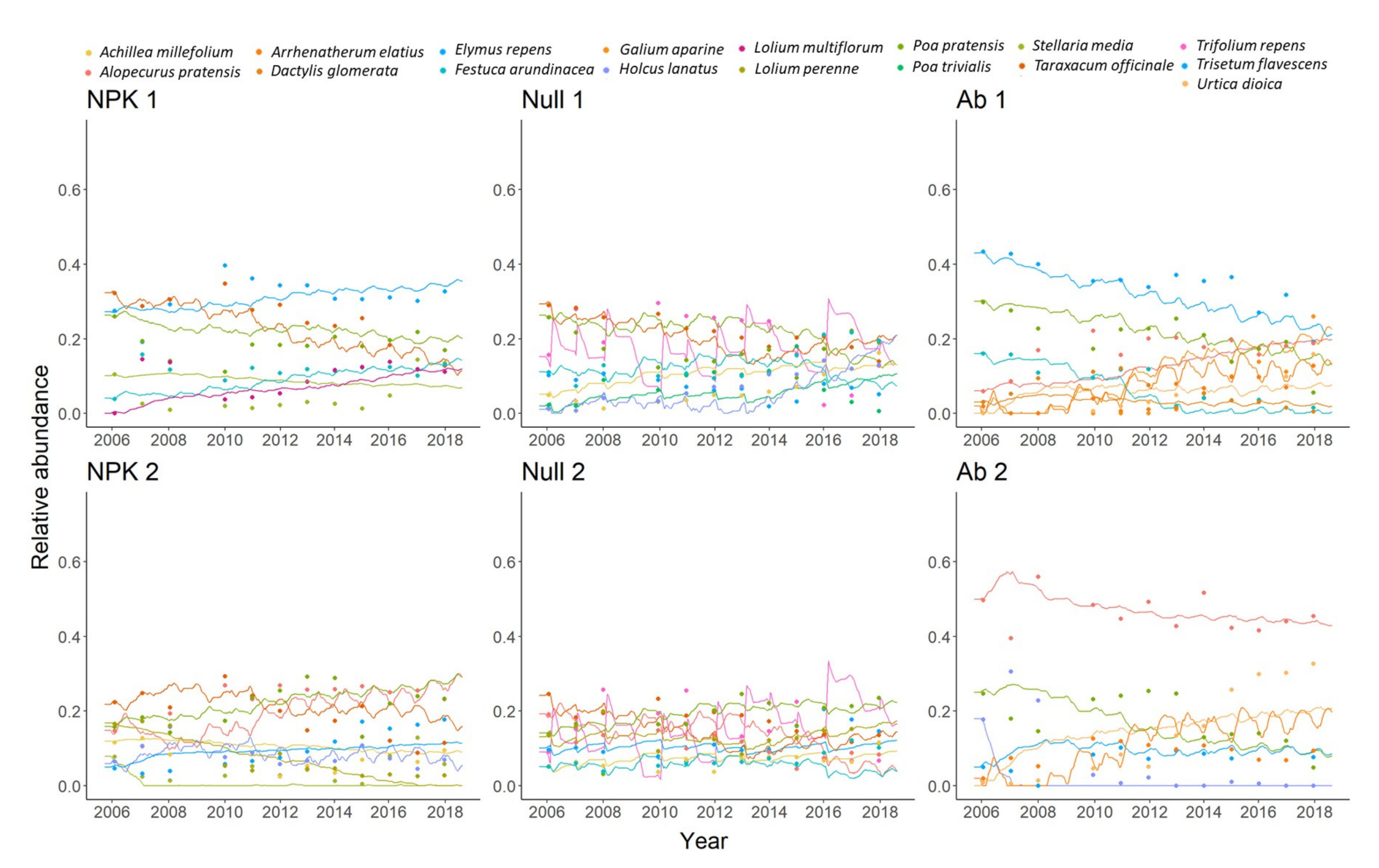
3.2. Evaluation of Modelling Solutions for Relative Abundances

3.2.1. Relative Abundance of Plant (Grass) Functional Types

Overall, the accuracy of ModVege-CoSMo in simulating the relative abundance of plant functional types was satisfactory (Table S12 in Supplementary Material, Figure 3). Type b had the highest correlation coefficient in block 2 NPK (R = 0.95), and type A had the lowest in block 2 abandonment (R = 0.04). However, the model accurately simulated the fluctuations of functional types with sufficient accuracy in all treatments, with RRMSE rarely >30% (i.e., types B and b in block 2 abandonment with 35.4% and 36.1%, respectively; Figure S10), and <10% in fertilised treatments (i.e., type A and type b in block 2, with 9.0% and 9.2%, respectively; Figure S6). The performance metrics improved at the community level (R > 0.70 and RRMSE < 25%).

3.2.2. Relative Abundance of Plant Species

The accuracy of ModVege-CoSMo in simulating the relative abundance of plant species was generally satisfactory (Table S13 in Supplementary Material, Figure 4). For the grasses, i.e., the dominant taxonomic group, the mean RRMSE is <40% (RMAE < 30%). Mean RRMSE~50% (RMAE~40%) calculated for forbs reflects the inaccuracies associated with two minor species (with three RRMSE values > 100%): G. aparine (block 1 abandonment; Figure S15) and S. media (NPK in both blocks; Figures S11 and S12). While both are present at the 4% limit on average (Table 2), G. aparine was notably absent in the first years of the study period (from 2006 to 2012), when the model estimated some presence of this species (Figure S15). Observed and simulated means for all grasses or forbs tend to converge, with a maximum departure of 6% abundance in block 1 Ab (0.90 versus 0.84 for grasses and 0.10 versus 0.16 for forbs).

Of grass species, F. arundinacea (RRMSE~38–56%) and L. perenne (RRMSE~24–34%) had the best R-values, respectively, in the abandoned plot of block 1 (R = 0.91) and in the fertilised plot of block 2 (R = 0.90). The worst R-value, observed for T. flavescens in block 2 Null (R = 0.04), reflects only a few data departing from the observations at the end of the simulation period (e.g., 2015, 2016, 2017; Figure S14), which are compatible with satisfactory error amounts (RRMSE = 36.4%, RMAE = 27.4%). The lowest simulation errors (RRMSE = 11.4%, RMAE = 8.5%) were obtained with E. repens in the abandonment of block 1 (Figure S15). Another dominant grass, P. pratensis (Figures S11–S16), shows mostly RRMSE < 30%—in NPK 1 and 2 (Figures S11 and S12), Null 2 (Figure S14) and Ab 1 (Figure S15)—or RRMSE < 50% in Null 1 (45.5%, Figure S13) and Ab 2 (36.2%, Figure S16). A dominant forb (absent in abandoned plots), T. officinale, shows RRMSE values < 25% (RMAE < 20%) in block 1 NPK (16.2% and 12.6%; Figure S11) and Null (12.4% and 9.8%; Figure S13) and in block 2 Null (22.8% and 18%; Figure S14), with RRMSE = 31.1% (RMAE = 24.1). Overall, the dynamics of T. repens in the unfertilised mown treatments were also reproduced (Figures S13 and S14), although with some discrepant values in the most recent years (RRMSE~62–77%; RMAE~49–62%). It was then shown that changes in ModVege-CoSMo accuracy are not related to the number of plant species in the community, with community RRMSE values ranging from ~30% to ~46% with six species (block 1 NPK and block 2 Ab) and from ~28% (block 2 Null) to ~52% (block 1 Null) with eight species.

The resulting feedback between plant species parameter values and modelled relative abundance of species (or types; Supplementary Material, Figures S17 and S18) permits a dynamic in defining community traits like, e.g., SLA (Figure 5) and maximum canopy height (Figure 6), whose values change during the simulation depending on the relative abundance of the species. For instance, the SLA values of the block 1 NPK community fluctuating around ~35 m² kg⁻¹ correspond to the value assigned to P. pratensis and E. repens (Supplementary Material, Table S6), dominant b-type grasses (with 31% and 17%, respectively; Table 2) with the environmental and management factors at work in the fertilised block 1 community. In this treatment, the modelled decline in community SLA is largely explained by the modelled (and observed) decline of T. officinale (Supplementary Material, Figure S11), a forb with high SLA (48 m² kg⁻¹; Supplementary Material, Table S7). Likewise, in block 2 NPK, dominated by the A-type grass A. pratensis (with 23% and SLA = 44 m² kg⁻¹; Table 2 and Supplementary Material, Table S7), community SLA declines below ~35 m² kg⁻¹ as a consequence of the decline of T. officinale (Supplementary Material, Figure S12).

With regard to the estimated values of maximum canopy height, their increase in the Ab community of block 1 reflects the (observed and simulated) increased abundance of two tall grass species, A. pratensis and A. elatius (Supplementary Material, Figure S15), which have calibrated maximum heights of 1.1–1.2 m (Supplementary Material, Table S10).

4. Discussion

4.1. Plant Biomass Simulation

Our results show that there is not always an adequate estimate of AGB by ModVege under different treatments, which also holds true with CoSMo-based modelling solutions. This indicates that the investigated grassland model is not yet sufficiently developed to capture the complexity of interactions between weather fluctuations, soil properties, floristic composition and the resilience of grassland communities to environmental stresses and management factors. However, discontinuous biomass measurements contain rather large uncertainties, mainly due to the spatial heterogeneity of grassland covers [66], which makes model evaluation difficult [67,68]. Even in this study, it is worth examining some issues with the experimental data, which may explain some of the discrepancies observed between the modelling solutions and the measurements. In 2008, the first biomass determination was postponed to the end of June (instead of the normal end of May; Table S2 in Supplementary Material) because the soil was waterlogged and the harvesting machine could not be put into the field earlier (due to the reduced bearing capacity of the soil). The biomass measurements were thus carried out on a canopy that had accumulated a lot of biomass at a very early stage of reproductive development. The high biomass observed in the first determination (after the clean-up determination) of 2008 (up to ~9 t DM ha⁻¹ in block 1 NPK, Table S2 in Supplementary Material), compared to other years, is thus more likely due to a late harvest (which allowed time for biomass accumulation) than to different weather conditions. Plants experienced some dry conditions early in the growing season in subsequent years with, for instance, a total reported precipitation of 161 mm from January to May in 2011 against ~300 mm in other years (from 211 mm in 2015 to 453 mm in 2016). In particular, in 2011, precipitation data indicate a relatively dry winter and spring (309 mm of total precipitation between November 2010 and June 2011), with a water deficit in April and soil water content remaining below average during May [69]. Thus, biomass production was lower than in other years in the first determinations of 2011, which is also one of the warmest years in the time-series, with three days with maximum air temperature > 35 °C detected at a nearby station [70]. This also likely reflects the lasting effects of the sequence of heatwaves that had occurred since 2009 [69].

Most problematic was the simulation of biomass in the abandonment treatment, a condition for which ModVege was not explicitly developed. Abandoned grasslands have complex vegetation structures that share environmental conditions with both open habitats and forests. At the study site, the abandoned grasslands are in an early succession stage, their vegetation structure is still more similar to open habitats than to forests, and we hypothesised that abandoned plots partly may act as managed grasslands. However, community similarity was relatively low, indicating that the dense sward found in abandoned plots created different environmental conditions (e.g., shade limiting light availability for emerging plants) compared to the mown grasslands. In particular, the vegetation cut at ground level included a lot of dead biomass components, which have increased over the years. The biomass sampled in summer (in July or August) was more similar to that of the mown grasslands, as it did not contain much dead biomass from the previous year’s growth or that of the current growing season (which is more present in the autumn sample). The simulations continue to indicate difficulties for all three modelling solutions to capture interannual variability in AGB (Table 4). Deviations from observations of up to ~3.7 t ha⁻¹ with ModVege standalone in 2018 in block 1 were however mitigated by the CoSMo-based solutions to ~2.8 t ha⁻¹. As well, the maximum deviation of ~3.0 t ha⁻¹ observed in block 2 in 2018 with ModVege standalone was reduced to ~2.0 t ha⁻¹ with CoSMo-based solutions.

Beyond the observational issues, the low modelling performance is not surprising, as simulations for grassland biomass are generally less accurate compared to cereal crops [71]. It is also a fact that the simulated biomass dynamics are essentially dissimilar between different grassland models, with shortcomings in the estimation of soil water content dynamics [72]. As well, ModVege simplifies plant growth simulation, with constant ratios of the above- to below-ground biomass allocation and plant water availability linked to fractional water content through a simple bucket approach used to assess the water reserve [49]. Taken together, these simplifications affect the accuracy of simulations of transpiration and soil water content. Consequently, to improve the performance of plant water demand and consumption simulation, a more detailed hydrological model should be integrated with the growth model.

Another important limitation of ModVege is that it assumes fixed values of the nutrition index, whereas, in reality, the availability of N and other nutrients varies with season, environmental conditions and management. In the context of the present study, the issue is relevant because N availability is highly dependent on management. The scope of the model thus needs to be extended to include important processes that determine the nutritional status of the plant community, such as a root compartment and components to explicitly simulate the availability of mineral and organic N to plants [73]. Since legume fixers represent an important component of grassland communities, contributing to maintaining high productivity under low N-fertiliser supply, consideration should also be given to including a model component to simulate symbiotic N fixation [74].

In addition, drought can cause changes in grassland dynamics through physiological responses [75]. The ability of some species to resist or avoid water stress through enhanced water uptake at low soil water potential [76,77], which is not currently taken into account in ModVege, may be important for understanding the disparity of responses observed in field studies.

Beyond eco-physiological responses, long-term changes related to grassland-community composition should be considered [78,79]. Here, the aim was not merely to assess the quality of AGB simulations by ModVege, but to evaluate this grassland model in comparison with solutions that introduce complexity in the modelling structure to represent plant dynamics (either species or functional types). The results are encouraging because, although the quality of the biomass simulations did not improve, it was not degraded by the complexity introduced. A pertinent point is that with CoSMo, it becomes possible for grassland simulators to obtain estimates of AGB while dynamically representing the relative abundance of plant species/types in mixed communities, a useful outcome for obtaining valuable information on a variety of ecosystem services provided by grasslands [80]. The use of a simplified plant-growth model structure, in conjunction with a plant dynamics module, proved useful as it allowed the properties of CoSMo to emerge, without interactions with the detailed biogeochemical processes of C and N cycles. CoSMo-like approaches could thus be more effective in simulating grassland biomass than in this study, as biophysical and biogeochemical issues are resolved.

4.2. Relative Abundance Simulation

The accuracy of ModVege-CoSMo in simulating the relative abundance of plant species in a community (RRMSE in the range ~28–52%; Supplementary Material, Table S13) was similar to that found by Movedi et al. [42] with CropSyst-CoSMo (~28–64%) and Soussana et al. [81] with GEMINI (51%), the latter (individual-centred model) being much more complex than CoSMo. The performances are also comparable to those of GRASSMIND (individual-based biogeochemical model [82]), which, however, was only applied to represent the vegetation cover of a limited number of species (mixture of two grass and one forb species).

With a total of 17 species simulated (up to eight per treatment, Table 2), this study goes beyond Movedi et al. [42], where a maximum of seven species were simulated together in a simplified grassland system (once-a-year mowing). In our study, seven CoSMo parameters (Table S9 in Supplementary Material) were added to 40 vegetation parameters in ModVege (24 functional type-specific parameters and 16 plant species-specific parameters; Tables S6 and S7 in Supplementary Material). In comparison, the generic crop model WOFOST [41] and the grassland model GEMINI [81] would need ~100 parameters to characterise each species and rapidly become increasingly complex as the number of species in the community increases, which obscures their interpretability and ultimately limits the applicability of the model.

Although limited to a single site, this study covers a variety of contrasting situations. They were not simulated with the same accuracy, which allows some strengths and weaknesses of the modelling framework to be identified. The satisfactory simulation of abundant grass species like E. repens and A. pratensis, but also F. arundinacea, L. perenne and the ubiquitous P. pratensis, is important in view of modelling studies in support of agronomic and ecological objectives. Despite its classification as a weedy perennial grass for row crops, E. repens (couch grass) has characteristics (erect stem growth habit, high feeding quality, vegetative reproduction through rhizomes, adaptation to a wide range of soil fertility and long seasonal growing periods) that make it an acceptable species for pastures [83], which may play a role for forage production and erosion control in northern temperate climates [84]. Its seeds are also eaten by several species of grassland birds [85]. A. pratensis (meadow foxtail) is also a pasture grass, usually mown before flowering to preserve its feed value, and used by some lepidopterans and other insects as a food plant [86]. F. arundinacea (tall fescue) is also an important forage crop under various fertility conditions, whose beneficial attributes for low-fertility soils are the result of a symbiotic association with an endophytic fungus, which increases soil C storage by limiting microbial and macro-faunal activity to decompose endophyte-infected organic matter inputs and by increasing C inputs through plant production [87]. L. perenne (perennial ryegrass) is an important perennial grass for turf grasses, globally one of the most important forage grasses, forming the basis of grassland production in temperate pastures as it has a low, dense vegetation with good regrowth and tillering [88]. The forage yield of P. pratensis (bluegrass) is lower compared to other temperate grasses, but it has a good regrowth capacity, responds well to intensive grazing, has good nutritional quality, is a food plant for various insects and is used in mixtures with taller species [89].

The performance indices highlight some inaccuracies in the estimates for two minor edible wild forbs, S. media (common chickweed) and G. aparine (cleavers), which are often considered weeds, and thus of no interest for fodder crops [90]. For instance, we obtained RRMSE values > 100% (Table S13 in Supplementary Material) for S. media in both fertilised plots and for G. aparine in the abandoned plot of block 1, which can be explained by the presence of a few data points deviating (with small absolute differences) from the general observed trend. In fact, although the performance metrics are not entirely satisfactory, the visualisation of the simulated species dynamics shown in the time-series plots is generally consistent with that of the observations (Figures S11, S12 and S15).

Our study also confirms other findings of a change in the abundance of some dominant species as an effect of abandonment [91,92]. For instance, this shift of species can be seen in the abandoned block 1 plot with a decline of important grass species (i.e., E. repens, F. arundinacea, P. pratensis) and an increase of the grass A. pratensis and forbs (i.e., G. aparine, U. dioica). Here, the important point is that the model was able to reproduce these dynamics (Figure S15). For the one legume species (white clover), present in unfertilised mown treatments, the spikes in the simulated lines (Figures S13 and S14) indicate that the N provided by the symbiotic fixation option of ModVege-CoSMo coupling needs to be refined.

These satisfactory simulations also support the expression of the distribution of plant trait values at the community level by averaging the trait values weighted by the respective abundance of each species (community weighted mean by Garnier et al. [93]), which functionally characterises plant communities in different environments in order to better understand community assemblages [94]. For the SLA, for instance, the simulated trends (here estimated from the dominant species) reflect those determined by Louault et al. [52] up to 2012, for the entire set of species present in the canopy.

5. Conclusions

The substantial agreement between the simulations and the experimental data, obtained in a set of environmental and management options at a representative site of semi-natural grasslands of central France, demonstrates that CoSMo is an appropriate approach for estimating the dynamic behaviour of plant species (or functional or taxonomic groups) in a community. Moreover, by contrasting trait values for individual species to aggregated values at the community level, we have dynamically estimated functional traits, which can support predictions of community composition along environmental gradients and provide a greater understanding of changing ecosystem functioning. This is important because CoSMo has fewer parameters than other modelling approaches representing plant abundance, is relatively easy to calibrate and allows the use of a single instance of a generic vegetation model. This study is one of the few to consider explicit and dynamic modelling of the relative abundance of plants in grassland communities and, although specific to the grassland model ModVege, holds potential for extension to other vegetation models of similar structure. However, the site-specific study and the situations used for modelling raise the need for a broader evaluation. First, this means that CoSMo-based ModVege may potentially be suitable for applications at other grassland sites if the model parameters are documented for those sites other than the one investigated here. Then, it is desirable to better understand the evolution of ecosystem functioning in the current context of global change in order to investigate whether measures of aggregate traits at the community level can be modelled at local scales, projected over the long term and upscaled across regions.

In conclusion, this study confirms that CoSMo-based solutions for grassland modelling can be easily implemented, although some background knowledge is required to parameterise each individual species/type in a grassland community. As the biophysical structure of CoSMo reflects important determinants of the functioning of grassland systems, we thus advocate its use to predict the behaviour of relevant grassland outputs, with three caveats. We first recommend further testing with grazing animals. Further tests are also required at a variety of sites, given the need to evaluate the CoSMo approach in contrasting biogeographic regions (e.g., the Mediterranean region where annual self-seeding species are dominant). Then, the present study highlights the need to orient grassland research towards the framing of dedicated functional trait measurements in the context of plant diversity and productivity observations for CoSMo-based modelling purposes. By advancing modelling to highlight the role of plant functional diversity in grassland performance, this study is a springboard for supporting agro-ecological farming. More research on these lines can be seen as the natural evolution of this study, with the aim of developing scalable solutions open to a wide range of grassland types, while addressing the issues of re-use and interconnection of model components.

References

1. Theau, J.-P.; Carrié, R.; Sirami, C.; Prud’homme, F. Grassland plant diversity: Definition. Dict. D’agroecologie. 2022. Available online: https://dicoagroecologie.fr/en/encyclopedia/grassland-plant-diversity (accessed on 7 October 2022).
2. Bengtsson, J.; Bullock, J.M.; Egoh, B.; Everson, C.; Everson, T.; O’Connor, T.; O’Farrell, P.J.; Smith, H.G.; Lindborg, R. Grasslands—more important for ecosystem services than you might think. Ecosphere 2019, 10, e02582. [Google Scholar] [CrossRef]
3. Perronne, R.; Mauchamp, L.; Mouly, A.; Gillet, F. Contrasted taxonomic, phylogenetic and functional diversity patterns in semi-natural permanent grasslands along an altitudinal gradient. Plant Ecol. Evol. 2014, 147, 165–175. [Google Scholar] [CrossRef] [Green Version]
4. Tilman, D.; Knops, J.; Wedin, D.; Reich, P.; Ritchie, M.; Siemann, E. The influence of functional diversity and composition on ecosystem processes. Science 1997, 277, 1300–1302. [Google Scholar] [CrossRef] [Green Version]
5. Tilman, D.; Reich, P.B.; Knops, J.M.H. Biodiversity and ecosystem stability in a decade-long grassland experiment. Nature 2006, 441, 629–632. [Google Scholar] [CrossRef]
6. Marquard, E.; Weigelt, A.; Roscher, C.; Gubsch, M.; Lipowsky, A.; Schmid, B. Positive biodiversity-productivity relationship due to increased plant density. J. Ecol. 2009, 97, 696–704. [Google Scholar] [CrossRef] [Green Version]
7. Kraft, N.J.B.; Godoy, O.; Levine, J.M. Plant functional traits and the multidimensional nature of species coexistence. Proc. Natl. Acad. Sci. USA 2015, 112, 797–802. [Google Scholar] [CrossRef] [Green Version]
8. Roscher, C.; Gubsch, M.; Lipowsky, A.; Schumacher, J.; Weigelt, A.; Buchmann, N.; Schulze, E.-D.; Schmid, B. Trait means, trait plasticity and trait differences to other species jointly explain species performances in grasslands of varying diversity. Oikos 2018, 127, 865. [Google Scholar] [CrossRef] [Green Version]
9. Chapin, F.S. Effects of plant traits on ecosystem and regional processes: A conceptual framework for predicting the consequences of global change. Ann. Bot. 2003, 91, 455–463. [Google Scholar] [CrossRef] [Green Version]
10. Ansquer, P.; Duru, M.; Theau, J.P.; Cruz, P. Functional traits as indicators of fodder provision over a short time scale in species-rich grasslands. Ann. Bot. 2009, 103, 117–126. [Google Scholar] [CrossRef] [Green Version]
11. Zheng, S.; Li, W.; Lan, Z.; Ren, H.; Wang, K. Functional trait responses to grazing are mediated by soil moisture and plant functional group identity. Sci. Rep. 2015, 5, 18163. [Google Scholar] [CrossRef]
12. Isbell, F.; Craven, D.; Connolly, J.; Loreau, M.; Schmid, B.; Beierkuhnlein, C.; Bezemer, T.M.; Bonin, C.; Bruelheide, H.; de Luca, E.; et al. Biodiversity increases the resistance of ecosystem productivity to climate extremes. Nature 2015, 526, 574. [Google Scholar] [CrossRef]
13. Díaz, S.; Lavorel, S.; de Bello, F.; Quétier, F.; Grigulis, K.; Robson, M. Incorporating plant functional diversity effects in ecosystem service assessments. Proc. Natl. Acad. Sci. USA 2007, 104, 20684–20689. [Google Scholar] [CrossRef] [Green Version]
14. Klumpp, K.; Soussana, J.-F. Using functional traits to predict grassland ecosystem change: A mathematical test of the response-and-effect trait approach. Glob. Change Biol. 2009, 15, 2921–2934. [Google Scholar] [CrossRef]
15. Lavorel, S. Plant functional effects on ecosystem services. J. Ecol. 2013, 101, 4–8. [Google Scholar] [CrossRef]
16. Quétier, F.; Lavorel, S.; Thuiller, W.; Davies, I. Plant-trait-based modeling assessment of ecosystem-service sensitivity to land-use change. Ecol. Appl. 2007, 17, 2377–2386. [Google Scholar] [CrossRef]
17. Lamarque, P.; Lavorel, S.; Mouchet, M.; Quétier, F. Plant trait-based models identify direct and indirect effects of climate change on bundles of grassland ecosystem services. Proc. Natl. Acad. Sci. USA 2014, 111, 13751–13756. [Google Scholar] [CrossRef] [Green Version]
18. Carrère, P.; Chabalier, C.; Landrieaux, J.; Orth, D.; Piquet, M.; Rivière, J.; Seytre, L. Une typologie multifonctionnelle des prairies des systèmes laitiers AOP du Massif Central combinant des approches agronomiques et écologiques. Fourrages 2012, 209, 9–22. (In French) [Google Scholar]
19. Cruz, P.; Duru, M.; Therond, O.; Theau, J.P.; Ducourtieux, C.; Jouany, C.; Al Haj Khaled, R.; Ansquer, P. Une nouvelle approche pour caractériser les prairies naturelles et leur valeur d’usage. Fourrages 2002, 172, 335–354. (In French) [Google Scholar]
20. Theau, J.-P.; Pauthenet, Y.; Cruz, P. Une typologie des espèces non graminéennes pour mieux caractériser la diversité et la valeur d’usage des prairies permanentes. Fourrages 2017, 232, 321–329. (In French) [Google Scholar]
21. Violle, C.; Navas, M.-L.; Vile, D.; Kazakou, E.; Fortunel, C.; Hummel, I.; Garnier, E. Let the concept of trait be functional. Oikos 2007, 116, 882–892. [Google Scholar] [CrossRef]
22. Michaud, A.; Andueza, D.; Picard, F.; Plantureux, S.; Baumont, R. Seasonal dynamics of biomass production and herbage quality of three grasslands with contrasting functional compositions. Grass Forage Sci. 2012, 67, 64–76. [Google Scholar] [CrossRef]
23. Duru, M.; Cruz, P.; Al Haj Khaled, R.; Ducourtieux, C.; Theau, J.-P. Relevance of plant functional types based on leaf dry matter content for assessing digestibility of native grass species and species-rich grassland communities in spring. Agron. J. 2008, 100, 1622–1630. [Google Scholar] [CrossRef]
24. Cruz, P.; Theau, J.P.; Lecloux, E.; Jouany, C.; Duru, M. Typologie fonctionnelle de graminées fourragères pérennes: Une classification multitraits. Fourrages 2010, 201, 11–17. (In French) [Google Scholar]
25. Jouven, M.; Carrère, P.; Baumont, R. Model predicting dynamics of biomass, structure and digestibility of herbage in managed permanent pastures. 1. Model description. Grass Forage Sci. 2006, 61, 112–124. [Google Scholar] [CrossRef]
26. Jouven, M.; Carrère, P.; Baumont, R. Model predicting dynamics of biomass, structure and digestibility of herbage in managed permanent pastures. 2. Model evaluation. Grass Forage Sci. 2006, 61, 125–133. [Google Scholar] [CrossRef]
27. Ehrhardt, F.; Soussana, J.-F.; Bellocchi, G.; Grace, P.; McAuliffe, R.; Recous, S.; Sándor, R.; Smith, P.; Snow, V.; de Antoni Migliorati, M.; et al. Assessing uncertainties in crop and pasture ensemble model simulations of productivity and N2O emissions. Glob. Change Biol. 2018, 24, e603–e616. [Google Scholar] [CrossRef] [Green Version]
28. Sándor, R.; Ehrhardt, F.; Grace, P.; Recous, S.; Smith, P.; Snow, V.; Soussana, J.-F.; Basso, B.; Bhatia, A.; Brilli, L.; et al. Ensemble modelling of carbon fluxes in grasslands and croplands. Field Crops Res. 2020, 252, 107791. [Google Scholar] [CrossRef]
29. Li, F.Y.; Snow, V.; Holzworth, D.R. Modelling the seasonal and geographical pattern of pasture production in New Zealand. N. Z. J. Agric. Res. 2011, 54, 331–352. [Google Scholar] [CrossRef] [Green Version]
30. Corre-Hellou, G.; Faure, M.; Launay, M.; Brisson, N.; Crozat, Y. Adaptation of the STICS intercrop model to simulate crop growth and N accumulation in pea-barley intercrops. Field Crops Res. 2009, 113, 72–81. [Google Scholar] [CrossRef]
31. Jégo, G.; Rotz, C.A.; Bélanger, G.; Tremblay, G.F.; Charbonneau, É.; Pellerin, D. Simulating forage crop production in a northern climate with the integrated farm system model. Can. J. Plant Sci. 2015, 95, 745–757. [Google Scholar] [CrossRef] [Green Version]
32. Thivierge, M.-N.; Jégo, G.; Bélanger, G.; Bertrand, A.; Tremblay, G.F.; Rotz, C.A.; Qian, B. Predicted yield and nutritive value of an alfalfa-timothy mixture under climate change and elevated atmospheric carbon dioxide. Agron. J. 2016, 108, 585–603. [Google Scholar] [CrossRef] [Green Version]
33. Wirth, S.B.; Taubert, F.; Tietjen, B.; Müller, C.; Rolisnki, S. Do details matter? Disentangling the processes related to plant species interactions in two grassland models of different complexity. Ecol. Model. 2021, 460, 109737. [Google Scholar] [CrossRef]
34. Moulin, T.; Perasso, A.; Gillet, F. Modelling vegetation dynamics in managed grasslands: Responses to drivers depend on species richness. Ecol. Model. 2018, 374, 22–36. [Google Scholar] [CrossRef]
35. Tilman, D. Resources: A graphical-mechanistic approach to competition and predation. Am. Nat. 1980, 116, 362–393. [Google Scholar] [CrossRef]
36. Moulin, T.; Perasso, A.; Calanca, P.; Gillet, F. DynaGraM: A process-based model to simulate multi-species plant community dynamics in managed grasslands. Ecol. Model. 2021, 439, 109345. [Google Scholar] [CrossRef]
37. Confalonieri, R. CoSMo: A simple approach for reproducing plant community dynamics using a single instance of generic crop simulators. Ecol. Model. 2014, 286, 1–10. [Google Scholar] [CrossRef]
38. Confalonieri, R.; Francone, C.; Cappelli, G.; Stella, T.; Frasso, N.; Carpani, M.; Bregaglio, S.; Acutis, M.; Tubiello, F.N.; Fernandes, E. A multi-approach software library for estimating crop suitability to environment. Comput. Electron. Agric. 2013, 90, 170–175. [Google Scholar] [CrossRef] [Green Version]
39. van Oijen, M.; Barcza, Z.; Confalonieri, R.; Korhonen, P.; Kröel-Dulay, G.; Lellei-Kovács, E.; Louarn, G.; Louault, F.; Martin, R.; Moulin, T.; et al. Incorporating biodiversity into biogeochemistry models to improve prediction of ecosystem services in temperate grasslands: Review and roadmap. Agronomy 2020, 10, 259. [Google Scholar] [CrossRef] [Green Version]
40. Stöckle, C.O.; Donatelli, M.; Nelson, R. CropSyst, a cropping systems simulation model. Eur. J. Agron. 2003, 18, 289–307. [Google Scholar] [CrossRef]
41. van Keulen, H.; Wolf, J. Modelling of Agricultural Production: Weather Soils and Crops; Pudoc: Wageningen, The Netherlands, 1986. [Google Scholar]
42. Movedi, E.; Bellocchi, G.; Argenti, G.; Paleari, L.; Vesely, F.; Staglianò, N.; Dibari, C.; Confalonieri, R. Development of generic crop models for simulation of multi-species plant communities in mown grasslands. Ecol. Model. 2019, 401, 111–128. [Google Scholar] [CrossRef]
43. Carrère, P.; Force, C.; Soussana, J.-F.; Louault, F.; Dumont, B.; Baumont, R. Design of a spatial model of a perennial grassland grazed by a herd of ruminants: The vegetation sub-model. In Grassland Science in Europe; Durand, J.-L., Emile, J.-C., Huyghes, C., Lemaire, G., Eds.; European Grassland Federation: Zürich, Switzerland, 2002; Volume 7, pp. 282–283. [Google Scholar]
44. Carrère, P.; Sosinski, E.E., Jr.; Louault, F.; Soussana, J.-F. Validation of a model simulating grassland vegetation dynamics using plant traits measured along a gradient of disturbance. In Grassland Science in Europe; Lüscher, A., Jeangros, B., Kessler, W., Huguenin, O., Lobsiger, M., Millar, N., Suter, D., Eds.; European Grassland Federation: Zürich, Switzerland, 2004; Volume 9, pp. 784–786. [Google Scholar]
45. Graux, A.-I.; Klumpp, K.; Ma, S.; Martin, R.; Bellocchi, G. Plant trait-based assessment of the Pasture Simulation model. In Proceedings of the 8th International Congress on Environmental Modelling and Software, Toulouse, France, 10–14 July 2016; Sauvage, S., Sánchez-Pérez, J.M., Rizzoli, A.E., Eds.; International Environmental Modelling and Software Society: Toulouse, France, 2016; Volume 2, pp. 518–525. [Google Scholar]
46. Schapendonk, A.H.C.M.; Stol, W.; van Kraalingen, D.W.G.; Bouman, B.A.M. LINGRA, a sink/source model to simulate grassland productivity in Europe. Eur. J. Agron. 1998, 9, 87–100. [Google Scholar] [CrossRef]
47. Bélanger, G.; Gastal, F.; Warembourg, F.R. Carbon balance of tall fescue (Festuca arundinacea Schreb.): Effects of nitrogen fertilization and the growing season. Ann. Bot. 1994, 74, 653–659. [Google Scholar] [CrossRef]
48. Hurtado-Uria, C.; Hennessy, D.; Shalloo, L.; Schulte, R.P.O.; Delaby, L.; O’Connor, D. Evaluation of three grass growth models to predict grass growth in Ireland. J. Agric. Sci. 2013, 151, 91–104. [Google Scholar] [CrossRef] [Green Version]
49. Calanca, P.; Deléglise, C.; Martin, R.; Carrère, P.; Mosimann, E. Testing the ability of a simple grassland model to simulate the seasonal effects of drought on herbage growth. Field Crops Res. 2016, 187, 12–23. [Google Scholar] [CrossRef]
50. Ruelle, E.; Delaby, L.; O’Donovan, M. La prévision de la croissance d’herbe en Irlande: Une information attendue, de l’éleveur au gouvernement. Fourrages 2021, 247, 33–39. (In French) [Google Scholar]
51. Ruelle, E.; Hennessy, D.; Delaby, L. Development of the Moorepark St Gilles grass growth model (MoSt GG model): A predictive model for grass growth for pasture based systems. Eur. J. Agron. 2018, 99, 80–91. [Google Scholar] [CrossRef]
52. Louault, F.; Pottier, J.; Note, P.; Vile, D.; Soussana, J.-F.; Carrère, P. Complex plant community responses to modifications of disturbance and nutrient availability in productive permanent grasslands. J. Veg. Sci. 2017, 28, 538–549. [Google Scholar] [CrossRef]
53. De Martonne, E. Nouvelle carte mondiale de l’indice d’aridité. Ann. De Géographie 1942, 51, 242–250. (In French) [Google Scholar] [CrossRef]
54. Diodato, N.; Ceccarelli, M. Multivariate indicator Kriging approach using a GIS to classify soil degradation for Mediterranean agricultural lands. Ecol. Indic. 2004, 4, 177–187. [Google Scholar] [CrossRef]
55. Grant, S.A. Resource description: Vegetation and sward components. In Sward Measurement Handbook, 2nd ed.; Davies, A., Baker, R.D., Grant, S.A., Laidlaw, A.S., Eds.; British Grassland Society: Reading, UK, 1993; pp. 69–97. [Google Scholar]
56. Piseddu, F.; Bellocchi, G.; Picon-Cochard, C. Mowing and warming effects on grassland species richness and harvested biomass: Meta-analyses. Agron. Sustain. Dev. 2021, 41, 74. [Google Scholar] [CrossRef]
57. Jackson, R.B.; Mooney, H.A.; Schulze, E.D. A global budget for fine root biomass, surface area, and nutrient contents. Proc. Natl. Acad. Sci. USA 1997, 94, 7362–7366. [Google Scholar] [CrossRef] [Green Version]
58. Sun, S.; Frelich, L.E. Flowering phenology and height growth pattern are associated with maximum plant height, relative growth rate and stem tissue mass density in herbaceous grassland species. J. Ecol. 2011, 99, 991–1000. [Google Scholar] [CrossRef]
59. Zhang, H.; Sun, Y.; Chang, L.; Qin, Y.; Chen, J.; Qin, Y.; Du, J.; Yi, S.; Wang, Y. Estimation of grassland canopy height and aboveground biomass at the quadrat scale using unmanned aerial vehicle. Remote Sens. 2018, 10, 851. [Google Scholar] [CrossRef] [Green Version]
60. Bourdôt, G.W. A Study of the Growth and Development of Yarrow (Achillea millefolium L.); Lincoln College, University of Canterbury: Canterbury, UK, 1980. [Google Scholar]
61. Ianovici, N.; Veres, M.; Catrina, R.G.; Pîrvulescu, A.M.; Tanase, R.M.; Datcu, D.A. Methods of biomonitoring in urban environment: Leaf area and fractal dimension. Ann. West Univ. Timisoara. Ser. Biol. 2015, 18, 169–178. [Google Scholar]
62. Gulías, J.; Flexas, J.; Mus, M.; Cifre, J.; Lefi, E.; Medrano, H. Relationship between maximum leaf photosynthesis, nitrogen content and specific leaf area in Balearic endemic and non-endemic Mediterranean species. Ann. Bot. 2003, 92, 215–222. [Google Scholar] [CrossRef]
63. Poorter, H.; de Jong, R. A comparison of specific leaf area, chemical composition and leaf construction costs of field plants from 15 habitats differing in productivity. New Phytol. 1999, 143, 163–176. [Google Scholar] [CrossRef]
64. Nölke, I.; Tonn, B.; Isselstein, J. Seasonal plasticity is more important than population variability in effects on white clover architecture and productivity. Ann. Bot. 2021, 128, 73–82. [Google Scholar] [CrossRef]
65. Bellocchi, G.; Rivington, M.; Matthews, K.; Donatelli, M. Validation of biophysical models: Issues and methodologies. A review. Agron. Sustain. Dev. 2010, 30, 109–130. [Google Scholar] [CrossRef] [Green Version]
66. Snow, V.; Rotz, C.A.; Moore, A.D.; Martin-Clouaire, R.; Johnson, I.R.; Hutchings, N.J.; Eckard, R.J. The challenges—and some solutions—to process-based modelling of grazed agricultural systems. Environ. Model. Softw. 2014, 62, 420–436. [Google Scholar] [CrossRef]
67. Vuichard, N.; Soussana, J.-F.; Ciais, P.; Viovy, N.; Ammann, C.; Calanca, P.; Clifton-Brown, J.; Fuhrer, J.; Jones, M.; Martin, C. Estimating the greenhouse gas fluxes of European grasslands with a process-based model: 1. Model evaluation from in situ measurements. Global Biogeochem. Cycles 2007, 21, GB1004. [Google Scholar] [CrossRef] [Green Version]
68. Gomára, I.; Bellocchi, G.; Martin, R.; Rodriguez-Fonseca, B.; Ruíz-Ramos, M. Influence of climate variability on the potential forage production of a mown permanent grassland in the French Massif Central. Agric. For. Meteorol. 2020, 280, 107768. [Google Scholar] [CrossRef]
69. Sándor, R.; Picon-Cochard, C.; Martin, R.; Louault, F.; Klumpp, K.; Borras, D.; Bellocchi, G. Plant acclimation to temperature: Developments in the Pasture Simulation model. Field Crops Res. 2018, 222, 238–255. [Google Scholar] [CrossRef]
70. Zwicke, M.; Alessio, G.A.; Thiery, L.; Falcimagne, R.; Baumont, R.; Rossignol, N.; Soussana, J.-F.; Picon-Cochard, C. Lasting effects of climate disturbance on perennial grassland above-ground biomass production under two cutting frequencies. Glob. Change Biol. 2013, 19, 3435–3448. [Google Scholar] [CrossRef] [PubMed]
71. Kollas, C.; Kersebaum, K.C.; Nendel, C.; Manevski, K.; Müller, C.; Palosuo, T.; Armas-Herrera, C.M.; Beaudoin, N.; Bindi, M.; Charfeddine, M.; et al. Crop rotation modelling—a European model intercomparison. Eur. J. Agron. 2015, 70, 98–111. [Google Scholar] [CrossRef]
72. Sándor, R.; Barcza, Z.; Acutis, M.; Doro, L.; Hidy, D.; Köchy, M.; Minet, J.; Lellei-Kovács, E.; Ma, S.; Perego, A.; et al. Multi-model simulation of soil temperature, soil water content and biomass in Euro-Mediterranean grasslands: Uncertainties and ensemble performance. Eur. J. Agron. 2017, 88, 22–40. [Google Scholar] [CrossRef] [Green Version]
73. Durand, J.-L.; Gonzales-Dugo, V.; Gastal, F. How much do water deficits alter the nitrogen nutrition status of forage crops? Nutr. Cycl. Agroecosyst. 2010, 88, 231–243. [Google Scholar] [CrossRef]
74. Fuchs, K.; Merbold, L.; Buchmann, N.; Bellocchi, G.; Bindi, M.; Brilli, L.; Conant, R.T.; Dorich, C.D.; Ehrhardt, F.; Fitton, N.; et al. Evaluating the potential of legumes to mitigate N2O emissions from permanent grassland using process-based models. Global Biogeochem. Cy. 2020, 34, e2020GB006561. [Google Scholar] [CrossRef]
75. Chaves, M.M.; Pereira, J.S.; Maroco, J.; Rodrigues, M.L.; Ricardo, C.P.P.; Osorio, M.L.; Carvalho, I.; Faria, T.; Pinheiro, C. How plants cope with water stress in the field: Photosynthesis and growth. Ann. Bot. 2002, 89, 907–916. [Google Scholar] [CrossRef] [Green Version]
76. Volaire, F. Plant traits and functional types to characterise drought survival of pluri-specific perennial herbaceous swards in Mediterranean areas. Eur. J. Agron. 2008, 29, 116–124. [Google Scholar] [CrossRef]
77. Volaire, F.; Lelièvre, F. Drought survival in Dactylis glomerata and Festuca arundinacea under similar rooting conditions in tubes. Plant Soil 2001, 229, 225–234. [Google Scholar] [CrossRef]
78. Gilgen, A.K.; Signarbieux, C.; Feller, U.; Buchmann, N. Competitive advantage of Rumex obtusifolius L. might increase in intensively managed temperate grasslands under drier climate. Agric. Ecosyst. Environ. 2010, 135, 15–23. [Google Scholar] [CrossRef] [Green Version]
79. Mariotte, P.; Vandenberghe, C.; Kardol, P.; Hagedorn, F.; Buttler, A. Subordinate plant species enhance community resistance against drought in semi-natural grasslands. J. Ecol. 2013, 101, 763–773. [Google Scholar] [CrossRef]
80. Weisser, W.W.; Roscher, C.; Meyer, S.T.; Ebeling, A.; Luo, G.; Allan, E.; Beßler, H.; Barnard, R.L.; Buchmann, N.; Buscot, F.; et al. Biodiversity effects on ecosystem functioning in a 15-year grassland experiment: Patterns, mechanisms, and open questions. Basic Appl. Ecol. 2017, 23, 1–73. [Google Scholar] [CrossRef]
81. Soussana, J.F.; Maire, V.; Gross, N.; Bachelet, V.; Pagès, L.; Martin, R.; Hill, D.; Wirth, C. GEMINI: A grassland model simulating the role of plant traits for community dynamics and ecosystem functioning. Parametrization and evaluation. Ecol. Model. 2012, 231, 134–145. [Google Scholar] [CrossRef]
82. Taubert, F.; Hetzer, J.; Schmid, J.S.; Huth, A. Confronting an individual-based simulation model with empirical community patterns of grasslands. PLoS ONE 2020, 15, e0236546. [Google Scholar] [CrossRef]
83. Amiaud, B.; Touzard, B.; Bonis, A.; Bouzillé, J.-B. After grazing exclusion, is there any modification of strategy for two guerrilla species: Elymus repens (L.) Gould and Agrostis stolonifera (L.)? Plant Ecol. 2000, 197, 107–117. [Google Scholar] [CrossRef]
84. Ringselle, B.; Bergkvist, G.; Aronsson, H.; Andersson, L. Under-sown cover crops and post-harvest mowing as measures to control Elymus repens. Weed Res. 2015, 55, 309–319. [Google Scholar] [CrossRef]
85. Snow, D.W.; Perrins, C.M. The Birds of the Western Palearctic; Oxford University Press: Oxford, UK, 1998. [Google Scholar]
86. Ružičková, H.; Banásová, V.; Kalivoda, H. Morava River alluvial meadows on the Slovak–Austrian border (Slovak part): Plant community dynamics, floristic and butterfly diversity—threats and management. J. Nat. Conserv. 2004, 12, 157–169. [Google Scholar] [CrossRef]
87. Franzluebbers, A.J.; Nazih, N.; Stuedemann, J.A.; Fuhrmann, J.J.; Schomberg, H.H.; Hartel, P.G. Soil carbon and nitrogen pools under low- and high-endophyte-infected tall fescue. Soil Sci. Soc. Am. J. 1999, 63, 1687–1694. [Google Scholar] [CrossRef] [Green Version]
88. McDonagh, J.; O’Donovan, M.; McEvoy, M.; Gilliland, T.J. Genetic gain in perennial ryegrass (Lolium perenne) varieties 1973 to 2013. Euphytica 2016, 212, 187–199. [Google Scholar] [CrossRef] [Green Version]
89. Martin, G.; Durand, J.-L.; Duru, M.; Gastal, F.; Julier, B.; Litrico, I.; Louarn, G.; Médiène, S.; Moreau, D.; Valentin-Morison, M.; et al. Role of ley pastures in tomorrow’s cropping systems. A review. Agron. Sustain. Dev. 2020, 40, 17. [Google Scholar] [CrossRef]
90. Defelice, M.S. Catchweed bedstraw or cleavers, Galium aparine L.—A very “sticky” subject. Weed Technol. 2002, 16, 467–472. [Google Scholar] [CrossRef]
91. Pavlů, L.; Pavlů, V.; Gaisler, J.; Hejcman, M.; Mikulka, J. Effect of long-term cutting versus abandonment on the vegetation of a mountain hay meadow (Polygono-Trisetion) in Central Europe. Flora: Morphol. Distrib. Funct. Ecol. Plants 2011, 206, 1020–1029. [Google Scholar] [CrossRef]
92. Jernej, I.; Bohner, A.; Walcher, R.; Hussain, R.I.; Arnberger, A.; Zaller, J.G.; Frank, T. Impact of land-use change in mountain semi-dry meadows on plants, litter decomposition and earthworms. Web Ecol. 2019, 19, 53–63. [Google Scholar] [CrossRef]
93. Garnier, E.; Cortez, J.; Billès, G.; Navas, M.-L.; Roumet, C.; Debussche, M.; Laurent, G.; Blanchard, A.; Aubry, D.; Bellmann, A.; et al. Plant functional markers capture ecosystem properties during secondary succession. Ecology 2004, 85, 2630–2637. [Google Scholar] [CrossRef]
94. Dubuis, A.; Rossier, L.; Pottier, J.; Pellissier, L.; Vittoz, P.; Guisan, A. Predicting current and future spatial community patterns of plant functional traits. Ecography 2013, 36, 1158–1168. [Google Scholar] [CrossRef]
Figure 1. Thermo-pluviometric regimes of the study-site according to the De Martonne-Gottmann aridity (yearly values).
Agronomy 12 02468 g001
Figure 2. Annual anomalies of aboveground biomass (AGB), observed and simulated with alternative modelling solutions in three treatments (NPK: fertilised; Null: unfertilised; Ab: abandoned) and two blocks (1, 2). Annual mean values of AGB: NPK 1: 2895 kg DM ha−1; NPK 2: 2477 kg DM ha−1; Null 1: 1417 kg DM ha−1; Null 2: 1197 kg DM ha−1; Ab 1: 5245 kg DM ha−1; Ab 2: 4683 kg DM ha−1.
Agronomy 12 02468 g002
Figure 3. Observed (dots) and ModVege-CoSMo simulated (lines) fluctuations in the relative abundance of plant (grass) functional types in three treatments (NPK: fertilised; Null: unfertilised; Ab: abandoned) and two blocks (1, 2). Type A: grass species of fertile environments, small, with early phenology and a short life span of the leaves; Type B: grass species of fertile environments, larger, with moderately early phenology and a longer leaf life than type A; Type b: grass species preferring relatively fertile environments but differing from the two previous groups in their late phenology. Graphs of the individual plant (grass) functional types are in (Supplementary Material Figures S6–S10).
Agronomy 12 02468 g003
Figure 4. Observed (dots) and ModVege-CoSMo simulated (lines) fluctuations in the relative abundance of plant species in three treatments (NPK: fertilised; Null: unfertilised; Ab: abandoned) and two blocks (1, 2). Graphs of the individual plant species are in (Supplementary Material Figures S11–S16).
Agronomy 12 02468 g004
Figure 5. Daily changes in the specific leaf area (SLA) of the community during the simulation period compared to the fixed values set for the plant species (coloured lines as in Figure 4) present in the community (horizontal lines, overlapping for the same values) for three treatments (NPK: fertilised; Null: unfertilised; Ab: abandoned) and two blocks (1, 2).
Agronomy 12 02468 g005
Figure 6. Daily changes in the maximum height of the community during the simulation period compared to the fixed values set for the plant species (coloured lines as in Figure 4) present in the community (horizontal lines, overlapping for the same values) for three treatments (NPK: fertilised; Null: unfertilised; Ab: abandoned) and two blocks (1, 2).
Agronomy 12 02468 g006