A Physiologically Based ODE Model for an Old Pest: Modeling Life Cycle and Population Dynamics of Bactrocera oleae (Rossi)

Abstract

The olive fruit fly Bactrocera oleae is one of the key insect pests infesting olive orchards in Mediterranean areas. Its coevolution with the olive tree, Olea europaea, made this pest highly specialized for this crop, being responsible for several yield reductions in terms of olive fruits and olive oil organoleptic properties. Monitoring is, to date, the main tool to assess the entity of infestations, but the increasing availability of biological information is making possible a quantitative interpretation of B. oleae’s biological traits in mathematical language. In this study, we aim to synthesize this plethora of information by applying a general physiologically based model theory of recent introduction. As a result, we obtained a parameterized model capable of describing B. oleae populations and with a high potential for implementation in Decision Support System programs. Besides the parameterization, model validation has been carried out in a three-year survey conducted in two representative productive areas of Sabina (Lazio, Central Italy). The model showed overall reliability in describing the field data trend, and it is a good starting point to be further improved.

1. Introduction

The olive fruit fly, Bactrocera oleae (Rossi) (Diptera: Tephritidae), is a key insect species of Olea europaea L. This pest is native to the Mediterranean basin [1,2], and it was accidentally introduced in new territories worldwide such as California, Mexico, the Canary Islands, and South Africa [2,3,4]. B. oleae is a primary and oligophagous injurious pest affecting olive fruits, where larvae feed and develop causing several economic losses (up to 15% of the yields) among producers [5,6]. The activity of this phytophagous reduces the yields because of the fruit dropout during the growing season, and consequently strongly decreases the olive oil quality in undesired alterations of the organoleptic characteristics [7,8,9,10]. Accordingly, this species affects the whole productivity chain related to olive producers, ranging from table olives to extra-virgin olive oil [3,11].

The harmfulness of B. oleae, as well as its high damaging potential, is known since ancient times [3], this is the reason why the scientific community has widely explored the biology of this species over the years. The life cycle comprises an egg, three larval instars, a pupal stage, adult males, and adult females, with a sex ratio of 1:1 (males: females) [6].

The thermal spectrum of B. oleae ranges from 10–12 to 30–32 °C, below and above which no egg hatching, adult survival, and larval development are observed [5]. According to the current literature, the optimal thermal conditions are centered around 25–26 °C, where the life cycle has an average duration of 50 days from the egg stage to the adult’s death [6]. In these conditions, B. oleae can complete up to 5 overlapping generations in the most suitable environments (e.g., the Middle East) with fluctuating population densities [12,13,14,15].

The occurrence of this pest in olive fields leads farmers to strictly monitor the populations and to carry out a set of control strategies based on different solutions. Treatments are commonly based on agrochemicals, mostly aimed to control the adult and larval stages, using active ingredients such as dimethoate or pyrethroids [3]. However, the increasing phenomenon of resistance to these active ingredients, as well as the ban that several pesticides have received by European regulators, led the scientific community to better explore alternative methods. Mass trapping [16], sterile male release [13], and natural enemies (predators and parasitoids) [3] were evaluated by different authors, showing promising results.

The basic concept behind any control strategy is the timing of the action, that is, to carry out treatments in the fields only when the population of the most susceptible life stage overcomes a fixed economic threshold [17,18]. Monitoring is the most common operation to evaluate the population variability/size over time in cultivated fields [19,20]. Different techniques allow us to focus on different key stages. B. oleae populations are usually monitored through (i) visual inspections of a given number of olives randomly collected in the olive orchards, which provide information on egg and preimaginal stages [21]; (ii) yellow chromotropic traps that collect both male and female adults [22]; and (iii) pheromone traps, that catch only adult males [3,22].

Despite the fact that monitoring is essential in the normal management of phytosanitary issues, it presents some critical aspects. Firstly, monitoring is a time-consuming activity that, for some techniques, requires a high level of expertise from technicians. Secondly, monitoring records the population trend from the past to the present, providing no information about the future evolution of infestations. Another issue is related to the low spatial and temporal resolution achieved by these methods [23]. This aspect can be confirmed by the Nyquist theorem [24] which relates to the sampling rate with the resolution that we can obtain during a data collection survey. Considering that monitoring is usually carried out on a weekly basis and in the spare points of the orchards, we can conclude that the actual monitoring practices are affected by a great loss of information. Accordingly, the low-resolution data obtained through monitoring makes it difficult to predict accurately (or constrains the precision) when the population peak of a target stage occurs, above all, in the continuously more adopted framework of precision agriculture [13]. In precision agriculture treatments are carried out only where and when strictly required, with a beneficial reduction of the inputs into cultivated fields and the environmental pollution [25]. A clearer indication of pest outbreaks is a fundamental requirement of precision agriculture, for this reason, the development of Decision Support Systems (DSS) tools based on mathematical models is always growing [26].

Mathematical modeling of pest species has the great potential of simulating further scenarios of infesting populations, being a powerful tool complementary to the actual monitoring techniques. In fact, through mathematical models it is possible to provide a schematic representation of insects’ life cycles, considering their development over time and through the life stages [27]. Being ectotherms, environmental parameters (e.g., temperature, relative humidity) are fundamental for a reliable representation of an insect’s species, given that life stage progress strongly depends on these factors [28,29,30].

Different authors [1,22,31,32,33] faced the problem of formulating and applying models describing the biology of B. oleae. The existing models describe both population dynamics and diffusion of this pest on large scales, but the recent information about the biology of the species, its relationship with the environmental temperature, and the availability of new models led us to extend the existing literature. Modeling of B. oleae to date stands at a low-level resolution in describing insect life cycle and its relationship with the environment. The current literature needs to be updated by considering, in a single model, two relevant aspects: a two-sex population and a detailed stage-density description related to environmental parameters and host plants.

Recently, Rossini et al. [27,34] introduced a new general mathematical model describing terrestrial arthropod populations, considering the biological features of the species as basic hypotheses. The model has been successfully applied in the case of the spotted-wing fly, Drosophila suzukii (Matsumura) (Diptera: Drosophilidae), and its potential can be extended to B. oleae as well. Moreover, biological information about the relationship between the development time of the species and environmental temperature published by Wang et al. [35] can be of great support to applying mathematical theory. The set of biological information is completed by the detailed review of Preu et al. [6], where accurate data about temperature-dependent fertility and mortality are reported. To the best of our knowledge, neither of these two datasets is still being used for modeling purposes.

This work aims to provide the first application of a recently published model to a key pest for olive cultivation, providing a new set of parameters, and a protocol of application that may be inserted in further DSS programs. The study is completed by field validation, where simulations are compared with data provided by different olive producers in the Sabina area (Lazio, Central Italy).

2. Materials and Methods

This section introduces the population density model describing B. oleae, the equations relating its life cycle with the environmental parameters, and how the parameters are estimated. The section is completed with a description of field trials, model solutions, and validation.

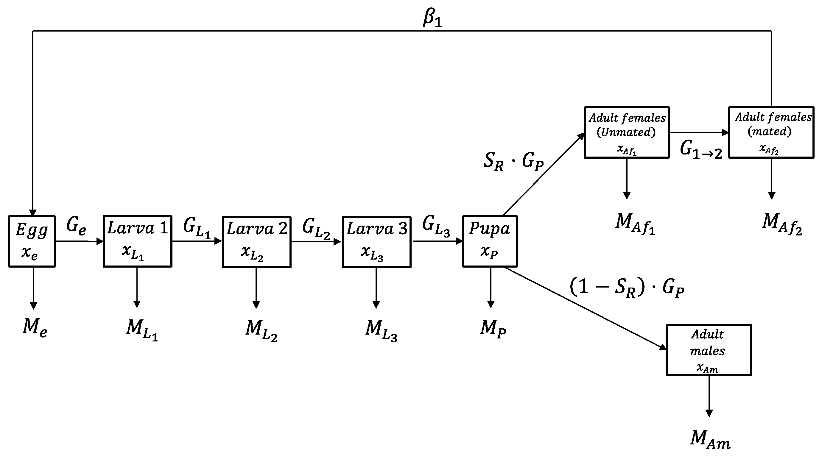
2.1. Population Density Model

The model considered in the present study directly comes from the modeling framework introduced by Rossini et al. [27,34], and from the biological assumptions behind B. oleae.

First, we need to know the number of stages that comprise the B. oleae life cycle. Each “identifiable” stage (i.e., the stages taxonomically defined) has an associated state $x_i\left(t\right)$, whose dynamics are described by an Ordinary Differential Equation (ODE). Accordingly, the whole life cycle is schematized by a system of chained ODEs. Based on biological information, B. oleae has an egg stage $x_e\left(t\right)$, three larval instars $x_{L1}\left(t\right)$, $x_{L2}\left(t\right)$, and $x_{L3}\left(t\right)$, a pupa stage $x_P\left(t\right)$, an adult male stage $x_{Am}\left(t\right)$, and two adult female stages: the non-mated females $x_{Anmf}\left(t\right)$ and the mated females $x_{Amf}\left(t\right)$.

The development of the individuals through the stages $i$ in relationship with environmental variables (i.e., temperature, as detailed in Section 2.2.1) is driven by specific “development rate functions”, hereby denoted $G_i\left(t\right)$.

Additional mortality $M_i\left(t\right)$, whose mathematical form will be discussed in Section 2.2.2, is associated with each stage as well. For the adult stages (male and females), this mortality is composed of two terms, as already hypothesized in the case of D. suzukii [27,36]: an adult longevity term $G_A\left(t\right)$ and an additional mortality term $M_A\left(t\right)$. In this way, we are taking into account the portion of individuals leaving the adult stage for different causes, considered independent of each other. Mathematically, adult mortality is formally written as:

$$M_A^{\prime }\left(t\right)=G_A\left(t\right)+M_A\left(t\right)$$

(1)

Little information is available about reproduction, particularly how many times adult females copulate during the life cycle. Benelli et al. [37] reported that B. oleae females are oligogamous and can mate 1–3 times during the life cycle, while adult males are polygamous and, once sexual maturity is reached, mate on a daily basis. However, it is still unclear if the oviposition is cyclic, namely, if the subsequent coupling occurs after the oviposition, or if it is continuous, that is a continued laying of eggs even though 1–3 coupling occurs. For modeling purposes, we assume that there is no cyclicity in reproduction and that females start to lay eggs continuously on olive fruits after the first coupling. According to this assumption, the rate of adult females that come from the mated to the non-mated substage after the oviposition is set to zero:

$$G_{1\leftarrow 2}\left(t\right)=0$$

(2a)

The polygamy of adult males, instead, leads us to suppose that there is a high probability for adult females and males to mate. Accordingly, we can avoid the dependence of fertility rates on the population density of males (for which, to the best of our knowledge, there is no information available to estimate some mathematical function) assuming that all the non-mated females become mated, except for the portion of dead. Mathematically speaking, this assumption leads to considering:

$$G_{1\to 2}\left(t\right)=1-M_A^{\prime }\left(t\right)$$

(2b)

Moreover, the general model of Rossini et al. [27,34] provides for the production of progeny from both adult female substages, extending the model’s suitability also to species where females have different oviposition behaviors as their age increases [38]. Given the division in non-mated and mated female substages assumed for B. oleae, only a single fertility rate function ${\beta }_1\left(t\right)$, detailed in Section 2.2.3, associated with the mated substage is considered.

If we add, to all the assumptions listed above, a sex ratio of $S_R=1/2$ we obtain the model adapted to the case of the olive fruit fly derived from the general framework of Rossini et al. [27]:

$$\{\begin{array}{c}\frac{d}{dt}{x}_e\left(t\right)={\beta }_1\left(t\right)x_{Amf}\left(t\right)-G_e\left(t\right)x_e\left(t\right)-M_e\left(t\right)x_e\left(t\right)\\ \frac{d}{dt}{x}_{L_1}\left(t\right)=G_e\left(t\right)x_e\left(t\right)-G_{L_1}\left(t\right)x_{L_1}\left(t\right)-M_{L_1}\left(t\right)x_{L_1}\left(t\right)\\ \frac{d}{dt}{x}_{L_2}\left(t\right)=G_{L_1}\left(t\right)x_{L_1}\left(t\right)-G_{L_2}\left(t\right)x_{L_2}\left(t\right)-M_{L_2}\left(t\right)x_{L_2}\left(t\right)\\ \frac{d}{dt}{x}_{L_3}\left(t\right)=G_{L_2}\left(t\right)x_{L_2}\left(t\right)-G_{L_3}\left(t\right)x_{L_3}\left(t\right)-M_{L_3}\left(t\right)x_{L_3}\left(t\right)\\ \frac{d}{dt}{x}_P\left(t\right)=G_{L_3}\left(t\right)x_{L_3}\left(t\right)-G_P\left(t\right)x_P\left(t\right)-M_P\left(t\right)x_P\left(t\right)\\ \frac{d}{dt}{x}_{Am}\left(t\right)=\left(1-S_R\right)G_P\left(t\right)x_P\left(t\right)-G_A\left(t\right)x_{Am}\left(t\right)-M_A\left(t\right)x_{Am}\left(t\right)\\ \frac{d}{dt}{x}_{Anmf}\left(t\right)=S_R{G}_P\left(t\right)x_P\left(t\right)-x_{Anmf}\left(t\right)\\ \frac{d}{dt}{x}_{Amf}\left(t\right)=\left(1-G_A\left(t\right)\right)x_{Anmf}\left(t\right)-M_A\left(t\right)x_{Anmf}\left(t\right)+\\ -M_A\left(t\right)x_{Amf}\left(t\right)-G_A\left(t\right)x_{Amf}\left(t\right)\end{array}$$

(3)

The compartmental scheme associated with model (3) is provided in Figure 1. It follows, in the next sections, a detailed description of all the rate functions involved in the model (3), as well as its parameterization. It is worth remarking, however, that very few pieces of literature report information accurately enough to quantitatively describe how environmental parameters different from temperature affect the life cycle of B. oleae. This is the reason why, for the sake of this work, the temperature is considered the main driving parameter. Even though it may seem a drastic approximation, it is common in modeling terrestrial arthropods, for instance, in [32,38,39,40,41,42,43].

2.2. Development, Fertility, and Mortality Rate Functions

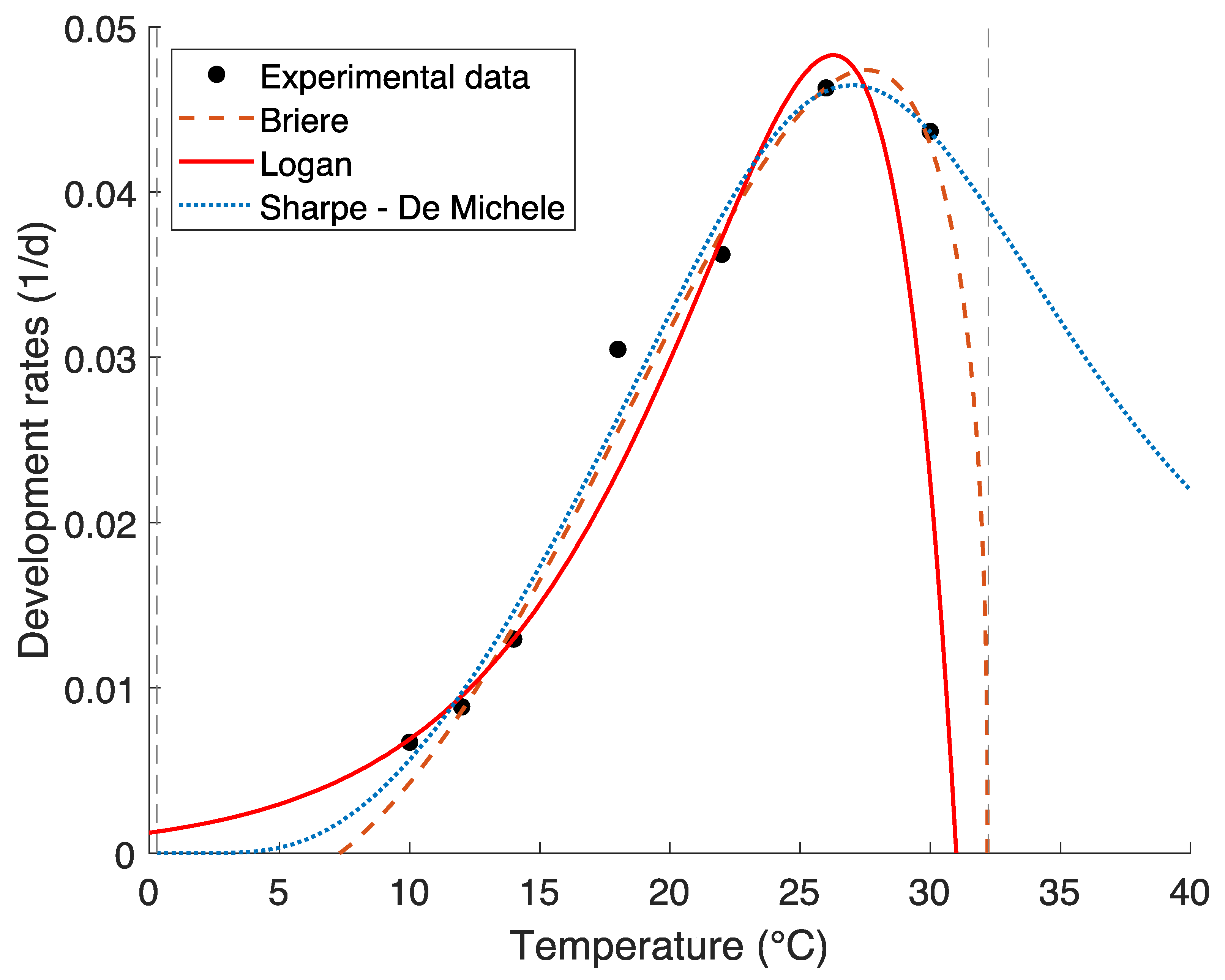
2.2.1. Development Rate Functions

Let us define the development rate functions that describe, in model (3), the temperature-driven development through the life stages and adult longevity as well. There are different equations in current literature relating to the environmental temperature, generally defined as $T\left(t\right)$, and the development rate $G\left[T\left(t\right)\right]$ [44,45,46,47].

The empirical nature of these equations makes it necessary to apply the a priori approach detailed in Rossini et al. [48]. This approach consists of estimating the parameters of all the main development rate functions available using the experimental and/or literature data available for the species under study.

The goodness of fit for each equation was assessed through a ${\chi }^2$-test and the coefficient of determination $R^2$. In this way we provided the best fitting function for B. oleae (also based on the dataset available), subsequently included in the model (3).

A preliminary screening was carried out to roughly check the best candidate functions. To not divert the attention from the main purpose of this work we only reported the development rate functions that provided the most interesting results for B. oleae, according to the literature data available.

Sharpe and De Michele development rate function [49,50,51]:

$$G\left[T\left(t\right)\right]=\frac{T\left(t\right)\cdot \exp \left(A-\frac{B}{T\left(t\right)}\right)}{1+ \exp \left(C - \frac{D}{T\left(t\right)}\right)+ \exp \left(E - \frac{F}{T\left(t\right)}\right)}$$

(4)

where $A$, $B$, $C$, $D$, $E$, and $F$ are parameters based on the enzyme kinetics [52,53].

Logan development rate function [54]:

$$G\left[T\left(t\right)\right]=\psi \left[\exp \left(\rho T\left(t\right)\right)-\exp \left(\rho T_M-\frac{T_M-T\left(t\right)}{\mathsf{\Delta }T}\right)\right]$$

(5)

where $\psi$ and $\rho$ are empirical parameters, $T_M$ (°C) is the upper-temperature threshold above which the development is theoretically not possible, and $\mathsf{\Delta }T$ (°C) is the temperature range between the maximum of Equation (3) and $T_M$.

Briere development rate function [55]:

$$G\left[T\left(t\right)\right]=a T\left(t\right) \left(T\left(t\right)-T_L\right){\left(T_M-T\left(t\right)\right)}^{\frac{1}{m}}$$

(6)

where $a$ and $m$ are empirical parameters, and $T_L$ and $T_M$ are lower and upper-temperature thresholds (°C), below and above which the development is theoretically not possible.

The parameters of Equations (4)–(6) were estimated using the dataset published by Wang et al. [35], where populations of B. oleae were reared at different constant temperatures. This dataset, however, covers only the egg-adult stage, without distinguishing among the preimaginal stages. Accordingly, obtaining a set of best-fit parameters specific to each life stage was not possible. We believe that this approximation does not impact the reliability of the model, as already shown in the case of other species [56,57]. Based on this hypothesis, we consider $G_{e }=G_{L1}=G_{L2}=G_{L3 }=G_P=G_A=G\left[T\left(t\right)\right]$ in the model (3).

A piece of additional information provided by Equations (4)–(6) is the optimal temperature for the development $T_{opt}$, i.e., the abscissa of their maxima [58]. This value can be calculated by placing the first order derivative of Equations (4)–(6) to zero, namely $\frac{d}{dt}G\left[T\left(t\right)\right]=0$ [55,56]. The errors associated with each $T_{opt}$ can be calculated from the standard errors of the best-fit parameters by using the propagation of uncertainty formula [36,52,59].

Calculations were carried out by the code already published in [20,56,60] and publicly available at https://hub.docker.com/r/lucaros1190/entosim/ (accessed on 14 August 2022). The algorithm provided for non-linear least squares fit that then, as a result, provided the best-fit parameters, and their respective standard errors.

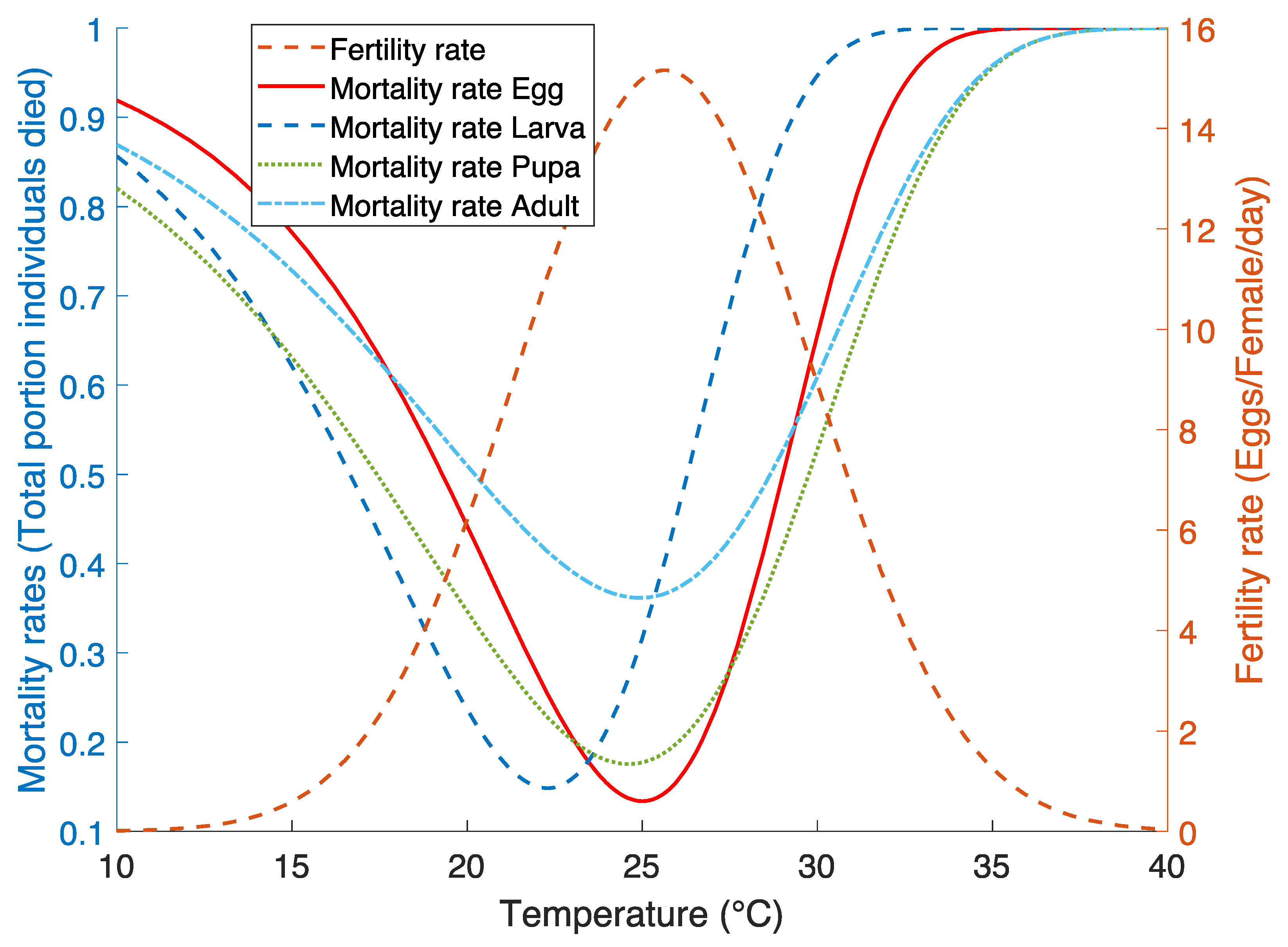
2.2.2. Mortality Rate Functions

As stated in Section 2.1, little information is available about the relationship between mortality and environmental parameters besides temperature in this species. Accordingly, we will focus only on this parameter and on its mathematical representation. We are aware that there is a plethora of sources of mortality besides temperature [41] such as, for instance, pest control actions in the case of cultivated fields. For the sake of this work, however, we have considered only olive orchards where B. oleae populations developed under natural conditions, without any control strategy applied.

Let us consider the survival rate introduced by Kim and Lee [61], and subsequently revised by Son and Lewis [39]. The normalized survival rate is defined as $S\left(t\right)$, and the mortality rate derives from the following definition $M\left(t\right)=1-S\left(t\right)$. This logical step leads to this temperature-dependent mortality rate function:

$$M_i\left[T\left(t\right)\right]=1-\left[k\exp \left(1+\frac{T_{MAX}-T\left(t\right)}{{\rho }_T}-\exp \left(\frac{T_{MAX}-T\left(t\right)}{{\rho }_T}\right)\right)\right]$$

(7)

where $k$ (dimensionless) and ${\rho }_T$ (°C) are empirical parameters, and $T_{MAX}$ (°C) is the temperature where survival is higher (and, accordingly, mortality is lower).

Mortality was described by Equation (7) in the case of the egg, larval instars, and pupa stages. Adult mortality was composed of two terms as indicated by Equation (1): the survival rate, expressed by the best-representing development rate function listed in Section 2.2.1, and Equation (7).

The number of stages covered by the mortality rate function (7) depends on the data available from the literature. A recent review by Preu et al. [6] allowed us to estimate 4 different sets of parameters for the function (7) describing egg $M_e\left[T\left(t\right)\right]$, larva $M_L\left[T\left(t\right)\right]$, pupa $M_P\left[T\left(t\right)\right]$, and adult $M_A\left[T\left(t\right)\right]$ temperature-dependent mortalities, respectively.

The literature dataset, however, refers to the total average mortality observed for each life stage. Accordingly, Equation (7) and the parameters estimated using the aforementioned dataset introduce a great overestimation of mortality. To overcome this problem, it is reasonable to suppose that the daily value $M_i\left[T\left(t\right)\right]$ (where $i$ is the life stage), evaluated based on the daily average temperature measured in the field, can be divided by the mean development time corresponding to the same daily temperature. In other words, considering that the development rate is defined as the inverse of the development time, the daily mortality rate is expressed by

$$M^{day}\left[T\left(t\right)\right]=M\left[T\left(t\right)\right]\cdot G\left[T\left(t\right)\right]$$

(8)

Equation (8) is valid in general, but it has been applied singularly to the egg, larva, pupa, and adult stages, according to the subdivision explained above in this section.

The process of parameter estimation is similar to development rate functions. A non-linear least squares fit was carried out using the script publicly available at https://github.com/lucaros1190/Mortality-survival (accessed on 14 August 2022). In particular, the script involved the scipy, NumPy, pandas, and matplotlib Python packages. As a result, we obtained the set of best fitting parameters specific for each above-mentioned stage, together with their standard errors. The goodness of fit was assessed through a ${\chi }^2$-test and the coefficient of determination $R^2$.

2.2.3. Fertility Rate Functions

Following the logic line of the previous sections, temperature-dependent fertility was modeled using the same Gaussian-like function that Ryan et al. [62] applied to D. suzukii:

$${\beta }_1\left[T\left(t\right)\right]=\alpha \left[\frac{\gamma +1}{\pi {\lambda }^{2\gamma +2}}{\left({\lambda }^2-\left({\left[T\left(t\right)-\tau \right]}^2+{\delta }^2\right)\right)}^{\gamma }\right]$$

(9)

The parameters of Equation (9), ($\alpha$, $\gamma$, $\lambda$, $\delta$, and $\tau$) are empirical with no biological meaning except for $\tau$, which is the optimal temperature (°C) for egg production. Data for the parameters’ estimation were instead retrieved by Preu et al. [6].

A non-linear least-squares fit was carried out through a Python script publicly available at https://github.com/lucaros1190/Fertility-rate (accessed on 14 August 2022), using the same packages listed in Section 2.2.2 As a result, we obtained the set of best fitting parameters with their standard errors. The goodness of fit was assessed through a ${\chi }^2$-test and the coefficient of determination $R^2$.

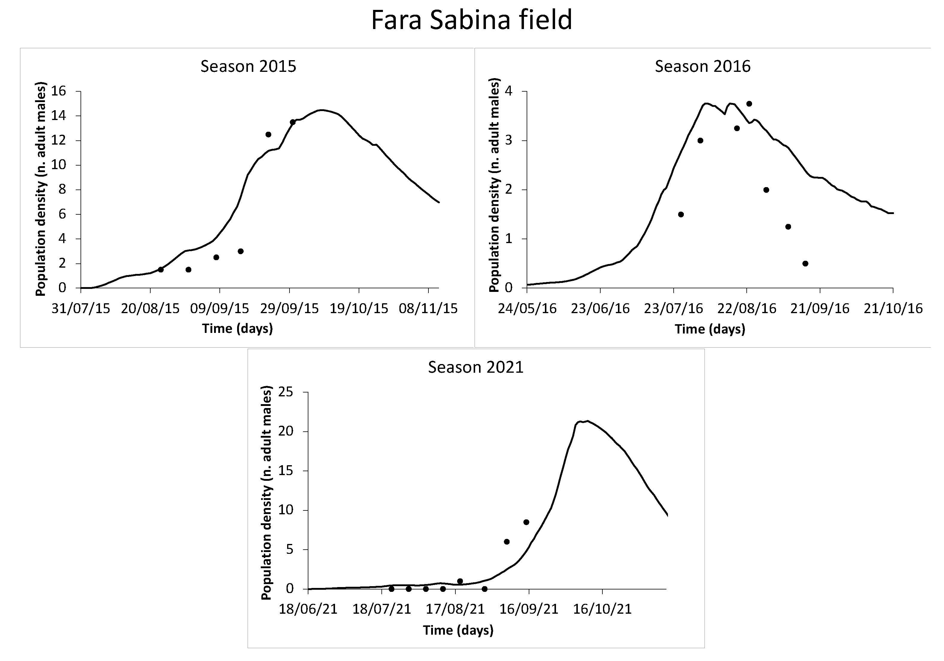
2.3. Field Data Collection for Model Validation

Validation of model (3) relied on field data collected by associations of farmers in the Sabina area, Lazio (Central Italy). This area is well known for its high-quality olive oil production. Despite population densities not being particularly high, B. oleae infestations represent the most serious threat to yields above all in seasons featured by warmer winters and rainy/wet summers. The recent increase of the annual mean temperatures, moreover, is causing a spread of the infestation in areas with a higher altitude as well, where B. oleae populations were sparse in the past years.

Each survey was carried out using pheromone delta traps (Isagro, Milano, Italy) that caught only adult males. Traps were deployed only during the olive ripening period, respecting a minimum distance of 30 m each, and were inspected weekly until the olive harvest. As the data was collected by farmers’ associations, the deployment of traps in the olive orchards was limited to the most susceptible period for olives.

To validate the model, orchards belonging to two representative areas were chosen, given their close position to two meteorological stations managed by the ARSIAL agency (https://www.siarl-lazio.it/, accessed on 14 August 2022). The first area was based on the meteorological station of Fara Sabina (Lazio, Italy) and the surveys selected for the model validation concerned the growing seasons of 2015 (traps from 17 August to 30 September), 2016 (traps from 19 July to 15 September), and 2021 (traps from 15 July to 15 September). The area was composed of two orchards (0.5 hectares per orchard, circa) each monitored by two traps (4 traps for the whole area). The second area, instead, was based on the meteorological station of Monteleone Sabino (Lazio, Italy) and the surveys selected for the model validation concerned the growing seasons of 2015 (traps from 27 June to 30 September), 2016 (traps from 19 July to 15 September), and 2017 (traps from 30 August to 14 November). The area was composed of 4 orchards (0.5 hectares per orchard, circa) each monitored by three traps (12 traps for the whole area). Meteorological stations provided the daily average temperatures calculated based on 48 daily acquisitions. Temperature series were subsequently inserted into model (3) to carry out simulations.

In each of the two areas, the weekly number of adult males provided by each trap was averaged to obtain a single value. Accordingly, traps belonging to each area equally contributed to the experimental population that was compared with simulations.

2.4. Model Evaluation and Comparison

Model (3), after the parameterization, was numerically solved using an ad hoc Python script publicly available at https://github.com/lucaros1190/ODE-bactrocera (accessed on 14 August 2022). The script provided, as input, daily average temperatures measured by the meteorological station, rate function (development, fertility, and mortality) parameters, sex ratio, and initial conditions. The output, on the other hand, was the population dynamics of each stage. Numerical solutions were calculated using the ODEint solver contained in scipy Python package, using the “RK45” (4th order Runge-Kutta) algorithm.

Model outputs were compared with field data by considering both the coefficient of determination $R^2$ and the ${\chi }^2$-value. ${\chi }^2$, in this case, assumes a meaning different from the classical statistical test, being considered as an indicator of the distance between simulated and experimental points [20,40,47,56,63,64]. It is worth pointing out that the higher the ${\chi }^2$-value, the lower the model reliability. However, in the case of high population densities, even a small difference can provide a large ${\chi }^2$-value [53], making the $R^2$ necessary to support model evaluation.

3. Results

Proceeding by order, the first step of the model application was the estimation of the development, mortality, and fertility rate function parameters. It was then possible to carry out simulations and compare them with field data.

3.1. Development Rate Functions

According to the procedure detailed in Section 2.2.1, the Briére equation was the most representative development rate function of the literature data available, followed by the Logan, and the Sharpe and De Michele equations. The best fitting parameters and their associated standard errors are listed in

Table 1. Development rate functions (4), (5), and (6) best-fit parameters and their associated standard errors (SE) for the whole egg-adult stage. Parameters were estimated using the dataset published by Wang et al. [35]. The goodness of fit was based on the ${\chi }^2$-test and its associated p-value, the coefficient of determination $R^2$, and the number of degrees of freedom (NDF). The best fitting functions are plotted in Figure 2.

Development Rate Function	Best Fit Parameters (±SE)		Goodness of Fit
Sharpe and De Michele (4)	$A$	$-12 \pm 2$	$R^2=0.988$
	$B$	$-200 \pm 80$	${\chi }^2=0.00119$
	$C$	$-7 \pm 2$	$P_{{\chi }^2}=0.0275$
	$D$	$-220 \pm 90$	$NDF=1$
	$E$	$-7 \pm 2$
	$F$	$-230 \pm 80$
Logan (5)	$\psi$	$\left(4.0 \pm 0.3\right)\cdot {10}^{-3}$	$R^2=0.775$
	$\rho$	$0.2056 \pm 0.0003$	${\chi }^2=0.0123$
	$T_M$	$31.000 \pm 0.005$	$P_{{\chi }^2}=3.61\cdot {10}^{-4}$
	$\mathsf{\Delta }T$	$4.599 \pm 0.005$	$NDF=3$
Briére (6)	$a$	$\left(4.6 \pm 0.2\right)\cdot {10}^{-5}$	$R^2=0.985$
	$T_L$	$7.23 \pm 0.07$	${\chi }^2=0.00129$
	$T_M$	$32.2 \pm 0.3$	$P_{{\chi }^2}=1.23\cdot {10}^{-5}$
	$m$	$2.5 \pm 0.1$	$NDF=3$

, while a plot of the best fitting functions is provided in Figure 2. The optimal temperatures for the development of the species, $T_{opt}$, calculated for the functions (4), (5), and (6) were consistent with each other, considering the error associated as well: $28 \pm 1$ °C for the Sharpe and De Michele, $26 \pm 8$ °C for the Logan, and $28.5 \pm 0.4$ °C for the Briére.

3.2. Mortality Rate Functions

The best-fit parameters of the mortality rate function (7), their associated errors, and the goodness of fit parameters are listed in

Table 2. Mortality rate function (7) best-fit parameters and their associated standard errors for egg, larva, pupa, and adult stage. The goodness of fit was based on the ${\chi }^2$-test, the coefficient of determination $R^2$, and the number of degrees of freedom (NDF). The best fitting functions are plotted in Figure 3.

Life Stage	Best Fit Parameters (±SE)		Goodness of Fit
Egg	$k$	$0.87 \pm 0.08$	$R^2=0.859$
	${\rho }_T$	$-4 \pm 1$	${\chi }^2=0.0045$
	$T_{MAX}$	$25.0 \pm 0.8$	$NDF=8$
Larva	$k$	$0.8 \pm 0.2$	$R^2=0.718$
	${\rho }_T$	$-4 \pm 1$	${\chi }^2=3.599$
	$T_{MAX}$	$22.0 \pm 0.9$	$NDF=6$
Pupa	$k$	$0.82 \pm 0.05$	$R^2=0.928$
	${\rho }_T$	$-6.0 \pm 0.5$	${\chi }^2=1.966$
	$T_{MAX}$	$24.6 \pm 0.5$	$NDF=8$
Adult	$k$	$0.6 \pm 0.1$	$R^2=0.775$
	${\rho }_T$	$-6 \pm 1$	${\chi }^2=1.743$
	$T_{MAX}$	$25 \pm 1$	$NDF=5$

, while the best-fitting functions are plotted in Figure 3. Additional plots comparing (stage by stage) the best fit function (7) with the literature dataset are provided as supplementary material. Equation (7) showed an overall reliable representation of survival data for egg, larva (without distinguishing between larval instars), pupa, and adult stages. The maximum of Equation (7) directly provided temperatures where mortality is the lowest: $25.0 \pm 0.8$ °C for egg, $22.0 \pm 0.9$ °C for larva, $24.6 \pm 0.5$ °C for pupa, and $25 \pm 1$ °C for adults. These values reflect the situation already described by development rate functions, even though in this case, data allowed a deeper distinction between the stages. Considering the errors associated, however, these values are inconsistent with the optimal temperature for the growth reported in Section 3.1 and deserve further discussion.

3.3. Fertility Rate Function

The best-fit parameters estimated for the fertility rate function (9), their associated standard errors, and the goodness of fit parameters are listed in

Table 3. Fertility rate function (9) best-fit parameters and their associated standard errors. The goodness of fit was based on the ${\chi }^2$-test, the coefficient of determination $R^2$, and the number of degrees of freedom (NDF). The best fitting function is plotted in Figure 3 and in the supplementary material.

Best Fit Parameters (±SE)		Goodness of Fit
$\alpha$	$7000 \pm 50$	$R^2=0.974$
$\gamma$	$70 \pm 20$	${\chi }^2=9.792$
$\lambda$	$50 \pm 2$	$NDF=4$
$\tau$	$25.6 \pm 0.4$
$\delta$	$7 \pm 1$

, while the best-fitting function is plotted in Figure 3 and in the supplementary material. Additional information is provided by the parameter $\tau$, the optimal temperature for egg production, having a value of $25.6 \pm 0.4$ °C. This optimal temperature is in accordance with the optimal values calculated for mortality, but not with the optimal temperature for development reported in Section 3.1.

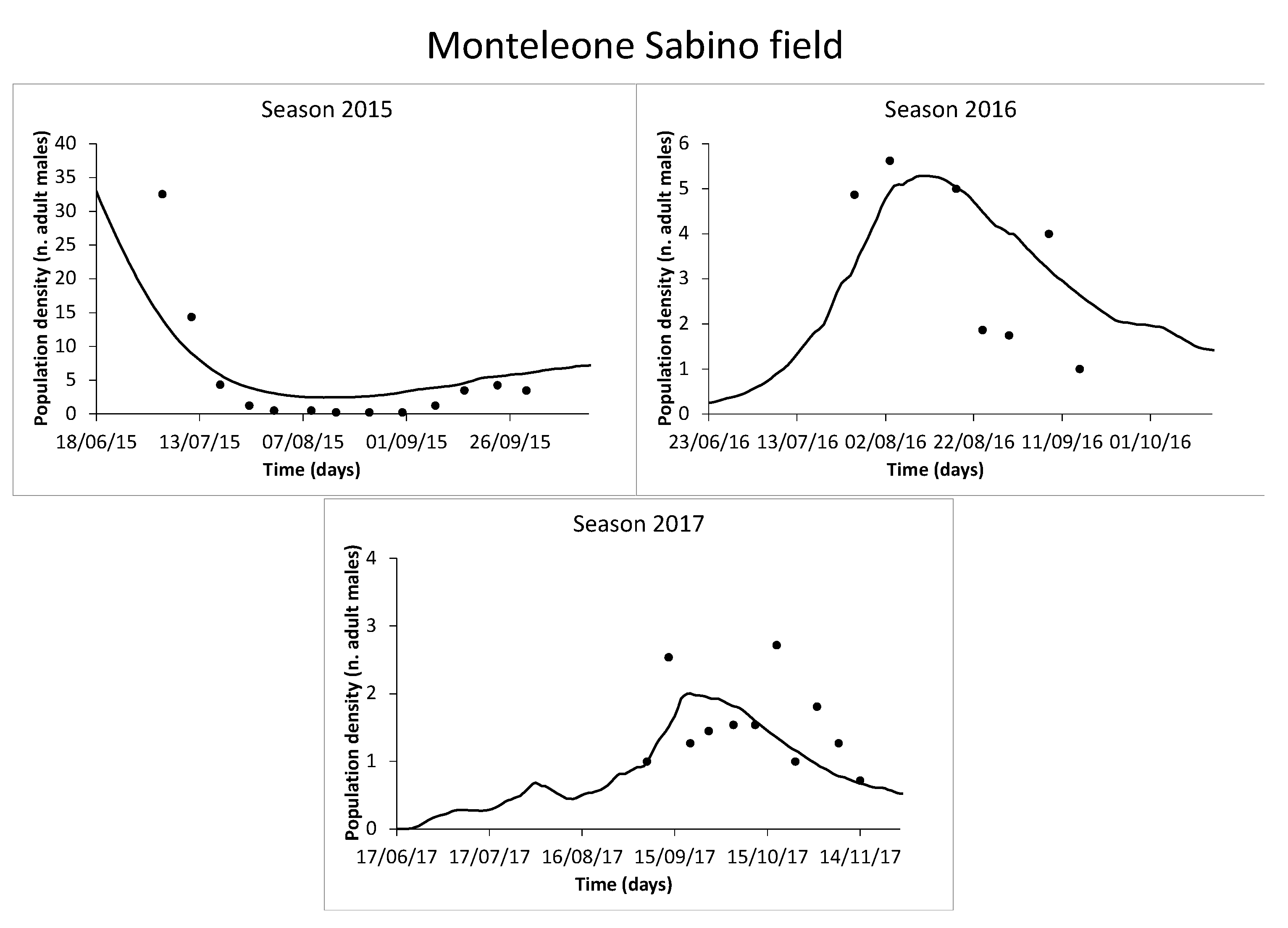
3.4. Model Validation

A resume of the model evaluation using the three-year data of the two experimental areas is reported in

Table 4. Resume of model validation in the three years and both experimental orchards.

Area	Year of Survey	Initial Conditions *	Time Range of Simulations	Model Evaluation Parameters
Fara Sabina	2015	$x_e\left(0\right)=2$	17 August–30 September	${\chi }^{2 }=4.23$
		$x_{Amf}\left(0\right)=4$		$R^2=0.86$
	2016	$x_{Amf}\left(0\right)=0.03$	19 July–15 September	${\chi }^2=3.62$
				$R^2=0.25$
	2021	$x_{Amf}\left(0\right)=0.2$	15 July–15 September	${\chi }^2=11.30$
				$R^2=0.66$
Monteleone Sabino	2015	$x_{Am}\left(0\right)=33$	27 June–30 September	${\chi }^2=126.30$
		$x_{Amf}\left(0\right)=1$		$R^2=0.43$
	2016	$x_{Amf}\left(0\right)=0.03$	19 July–15 September	${\chi }^2=4.89$
				$R^2=0.84$
	2017	$x_{Amf}\left(0\right)=0.03$	30 August–14 November	${\chi }^2=0.77$
				$R^2=0.47$

* For the sake of simplicity only initial conditions different from 0 were reported. It is implicitly assumed that all the state variables not reported are set to zero.

. Proceeding by order, the focus is now on the Fara Sabina area (Figure 4). Overall, the male population density was low, particularly in season 2016. During season 2015, an increasing profile was observed until the end of the samplings. An experimental maximum of the population was reached on 30 September, while the simulation suggested a peak of the population on 8 October with a subsequent decrease in the population. The situation was different the year after, 2016, when an increasing-decreasing profile was assessed in field data, with a maximum on 23 August. Two maxima, instead, were suggested by the simulation, more specifically on 5 August and 15 August, respectively. Season 2021 was similar to 2015 overall, with an increasing population until the end of the survey and a maximum value recorded on 15 September. In this case, simulations suggested a continuous increase of the population until reaching a maximum on 10 October.

The second part of the results concerns the Monteleone Sabino area (Figure 5). The overall male population density assessed was similar to the Fara Sabina area, except for season 2015 when the highest value of the survey was recorded. Proceeding by order, season 2015 had a decreasing population profile, starting from the maximum value recorded on 4 July and gradually decreasing until the end of the survey, making it necessary to set the initial conditions of the model as indicated in Table 4. Simulations faithfully described this trend, showing a slight increase in the final part of the season. Season 2016 showed an increasing-decreasing profile with a maximum recorded on the 3 August. Simulations, in this case, reported a maximum on 11 August, close to what was experimentally observed. The last season considered for the Monteleone Sabino area, 2017, reported a profile similar to 2016, with comparable population densities but with an overall higher variability. Two maxima were observed on 13 September and 18 October, respectively, while the simulation reported a single maximum of the population on 20 September.

4. Discussion and Conclusions

This study introduced the first application of a general physiologically-based ODE model to describe Bactrocera oleae populations. Overall, a synthetic mathematical representation of both existing literature data and field data provided a better quantitative interpretation of some biological aspects of this species, along with a model that faithfully describes its life cycle.

4.1. Comparison with Other Existing Models

Modeling the pests associated with olive cultivations is gaining relevance in the last few years. Pappalardo et al. [65] have recently published a model describing Prays oleae (Bernard) (Lepidoptera: Praydidae) population dynamics considering the interaction with two natural enemies. Even though the model does not consider the subdivision in life stages as the model (3), it shows how ODE systems are suitable to describe insect populations. Other interesting theoretical results were obtained by Brunetti et al. [66] about a three-actor model describing epidemics of Xylella fastidiosa in relationship with host plants and its vector Philaenus spumarius (L.) (Hemiptera: Aphrophoridae). These models are a classical example of how different field scenarios can be reproduced in silico. Besides the mathematical background, our model completely shares the final application that models should have, that is the representation of a plausible situation in which farmers may act.

Modeling has the power of reproducing different scenarios based on the parameters inserted and may actively support the planning of olive orchard management. The models existing in literature to describe B. oleae are mathematically different from the model (3). Pucci et al. [22,31,67] proposed a model that indicates a risk based on average temperature values and females caught with chromotropic traps. Given its simplicity and its reliability in different areas of South and East Europe, this model has been employed for many years. However, the model of Pucci et al. is formulated based on historical data on B. oleae flights (strictly related to the particular environment of acquisition) and does not report any information about population dynamics. According to these hypotheses, the model loses its reliability in areas with climate features too far from the area where historical data for the parameter estimation were collected, or in areas mostly affected by recent climate changes.

An analogous model describing the maturation time of B. oleae based on a degree-day approach was proposed by Petacchi et al. [33,68], with successful validations in different areas of the Liguria region (Northern Italy). This model, however, does not provide any information about population density in each life stage, hence being affected by the same issue as Pucci et al.’s model.

To the best of our knowledge, the only two existing models describing the population dynamics of B. oleae were introduced by Gutierrez et al. [1] and Gilioli and Pasquali [32]. Proceeding by order, Gutierrez et al. [1] considered a distributed delay model [69,70] to project the potential suitability of B. oleae in California and Italy under a climate change scenario. We can consider model (3) as a generalization of the model of Gutierrez et al., which also adds the possibility of describing male populations. The spatialized version of the model (3) [34], moreover, will open the door to further implementation in GIS systems, even though to date there is no quantitative information about B. oleae flight and spreading strategy.

Gilioli and Pasquali [32], instead, described the dynamics of B. oleae populations using a second-order partial differential equation subsequently discretized to be reduced to a system of ODEs [71]. Even though this approach looks similar to model (3), only female populations are considered, and there is no possibility of eventually introducing the density dependence on male populations into fertility/reproduction rates.

Based on these considerations, we may say that model (3) includes all the characteristics of the existing models, going beyond the state current state of the art and being a good candidate for further implementation in DSS. However, the theory still needs to be improved and validated in contexts different from Central Italy. Testing the model in places with different climates and infestation levels would be a great opportunity to better explore the range of validity of the model.

An additional aspect worthy of investigation is the relationship between the species and the host plant. The general structure of the ODE model allows the inclusion of transition rates that depend on food availability as well, besides environmental parameters. The presence of the host plant in model (3) can be of great support to agronomical practices, this is the reason why a further investigation should be directed in this direction. Pest abundance and olive fruits attractivity are two relevant pieces of information in setting up control strategies, as well as in better identifying the timing of the action.

4.2. Development, Mortality, and Fertility Rates

Even though the Briére Equation (6) was the best fitting function for the data published by Wang et al. [35], helpful quantitative information was derived from the other equations as well. The lower temperature threshold for B. oleae development, $T_L$, is explicitly considered only by the Briére equation. However, the maximum thermal threshold, $T_M$, is contained in both the Briére (6) and Logan (5) equations, allowing a comparison between values. In particular, the best-fit $T_M$ associated with Equations (5) and (6) are close to each other; however, they cannot be considered similar according to the standard errors of the best-fit values.

It may be reasonable to ask which is the most reliable $T_M$ value. The best fitting development rate function, among (4)–(6), to simulate B. oleae populations through model (3) has been identified by a limited life tables literature dataset. In the alternative, we may divide the total temperature range into different sub-ranges, selecting the best fitting function for each sub-range [56,59]. Even though this operation may provide a better interpretation of the life tables dataset, it is effective only if a large amount of data to test the different equations in the various sub-ranges is available. Life tables data of B. oleae provided by Wang et al. [35] consisted only of average values of the development times at different constant temperatures (there were no raw datasets accessible) and were not specific for each life stage (e.g., for mortality rates). Based on this precondition, it is not worth using more complex methods if the foreseen result is similar [57]. However, this approach would be helpful to discriminate, in future works, which is the most reliable $T_M$: it will be related to the best fitting function, between (5) and (6), for the high temperatures range.

From an agronomic point of view, $T_M$ is helpful biological information in choosing olive varieties to place in new orchards. Based on the climate conditions of the area of interest the best compromise would be to have the olive fruit ripening close to the hottest temperature conditions. Based on the development rate functions, in fact, with this strategy, we may have a shift in pest and fruit development, with a potential reduction of the control actions.

The second piece of quantitative information comes from the Logan equation, more specifically from the parameter $\mathsf{\Delta }T$. This parameter indicates the temperature range in which the development of the species switches from its maximum to zero in case of high temperatures (from the optimal temperature to $T_M$). According to our results, an increase of 4 °C above optimum temperature causes a strong stage-development reduction. There is always, in real cases, a small probability that B. oleae develops in temperatures higher than the maximum threshold as well [72]. However, the quantitative information provided by this part of the study reflects the behavior generally observed in the middle of summer in many Mediterranean areas [73,74,75], including the Sabina area. Temperature affects the development of B. oleae more in areas when warmer summers occur [73,76]. In particular, high temperatures provoke a consistent reduction in adult female fertility and summer dormancy, leading the third instar larvae to migrate from olive fruits to soil and pupate [74,76]. On the other hand, temperature plays a fundamental role in wintertime [6,75], when B. oleae overwinters both as facultative-reproduction adults and soil-pupae [33]. It has been shown that in areas featured by warmer winters, the populations occurring in the following spring are higher [77] requiring, de facto, more control actions. In this study, we have not considered any winter or summer dormancy/quiescence or diapause, this is the reason why we have assumed that below and above the minimum and maximum thermal limit, respectively, the development is simply set to zero.

More detailed information, despite being affected by some of the above-mentioned problems, comes from the mortality rate function. The dataset was more specific for life stages, but the information was concerning the total portion of dead individuals, not their daily value. The assumption of obtaining the number of dead individuals per day through development rate functions, as indicated in (8), gave promising results, according to the model evaluation. We are aware that development rate functions have different coverage of life stages from mortality ones, but a certain degree of flexibility in the model assumptions is often required in the case of scarcity of data [26]. It is worth reminding that in the great part of the physiologically based models all the rate function (development, mortality, and fertility) parameters are estimated using average data [50]. In other words, we are just modeling the average population behavior, without going into detail about the intra-population genetic variability responsible for the distribution of the individuals around average values [78]. Biologically speaking, most physiologically based models existing in literature [38,41,79,80,81,82], including the model (3), implicitly assume that all the individuals of the population have the same behavior.

A piece of quantitative information worthy of discussion provided by our results is the optimal temperature where mortality is lower, $T_{MAX}$. Egg, pupa, and adult stages have a comparable thermal optimum for survival, considering the errors associated with the best fitting parameters. Larvae, instead, seem to have a lower tolerance to warm temperatures, and this may justify the high mortality rate during warmer seasons that different authors have reported [73].

Overall, temperature values where mortality is lower are slightly different from each other and not comparable with the optimal temperature for development indicated by development rate functions. If in this comparison we include the optimal temperature value for fertility calculated through Equation (9), we may also suppose that the optimal temperature for development should be slightly lower. This difference needs further investigation in future studies, for example by estimating stage-specific development rate functions and comparing results.

4.3. Population Trend and Model Validation

The model showed overall reliability in representing field population trends, even though in two growing seasons (2016, Fara Sabina area and 2017, Monteleone Sabino area) simulations did not completely fit the experimental data. Part of this discrepancy may be associated with the overall lower populations assessed during the growing seasons, which may lead to a less defined trend. Another reason behind this discrepancy may be the delayed flight of females with respect to males [67], which leads to suppose that future works should be focused on life tables considering both sexes, as already suggested by Chi et al. [83,84].

To improve model (3) parameterization, future works should focus on the effect that relative humidity and the amount of water on olive plants have on development, mortality, and fertility rates. The fragmented information in the current literature [85,86] suggests that relative humidity plays a crucial role in the development of the species during the summer period, reducing mortality and pupation time in the soil [3]. It has been observed that during hot and dry growing seasons, the incidence of infestations is lower [72], and this is a relevant aspect to include in the model (3). Moreover, plant susceptibility has been observed to depend not only on the cultivar [5,87,88] but also on irrigation [89,90]. The higher susceptibility of irrigated plants, in fact, may be due to the higher suitability of olive fruits for female oviposition and larval development. This leads one to suppose that in the case of dry summers and irrigated olive orchards, mortality rate functions should be corrected to not overestimate the daily losses of individuals.

Despite the above-mentioned problems and scope for improvements, model (3) showed to be a good candidate for further implementations in DSS, even though additional investigations are still required. One of the peculiarities of model (3) is the possibility of being supported by optimization algorithms (e.g., Kalman filter, particle filter) that update the estimations based on measurement data. Some promising results have been presented by Bono Rossello et al. [91] from a theoretical point of view, and future applications in real cases will be possible soon. Monitoring data, in this case, became an active part of the modeling tool, partially compensating for the gap in knowledge affecting rate functions’ parameterization.

If supported by optimization algorithms, model (3) may potentially help to plan data collection campaigns. The number of traps, as well as the time range between two trap inspections, can be increased or decreased based on the degree of reliability required by the model. This degree of reliability can be represented by an ad hoc equation that the general structure of the model (3) is ready to include. This future direction will bring a tool compatible with the precision agriculture framework, where measurements and model estimations support pest control.

The purpose of using monitoring data collected directly by associations of farmers to validate the model (3) in an open loop wanted to be also a preliminary test of the suitability of this dataset for modeling purposes. Even though simulations were capable of reproducing the population trend, it was not possible to assess the reliability of the model for longer time ranges. On the other hand, future model optimization (e.g., Kalman filter, particle filter) will require a change in the way of carrying out monitoring, and simulations may also be beneficial to understand if and when monitoring should be conducted.

This study proposed an application of a general pest modeling theory in the case of an injurious pest for olive cultivations. We believe that the methodology and the results represent a step forward with respect to the current literature while also being a new starting point for further improvements.

References

1. Gutierrez, A.P.; Ponti, L.; Cossu, Q.A. Effects of climate warming on olive and olive fly (Bactrocera oleae (Gmelin)) in California and Italy. Clim. Change 2009, 95, 195–217. [Google Scholar] [CrossRef]
2. Baratella, V.; Pucci, C.; Paparatti, B.; Speranza, S. Response of Bactrocera oleae to different photoperiods and temperatures using a novel method for continuous laboratory rearing. Biol. Control 2017, 110, 79–88. [Google Scholar] [CrossRef]
3. Daane, K.M.; Johnson, M.W. Olive fruit fly: Managing an ancient pest in modern times. Annu. Rev. Entomol. 2010, 55, 151–169. [Google Scholar] [CrossRef]
4. EPPO. EPPO Global Database. Available online: https://gd.eppo.int/taxon/ (accessed on 14 August 2022).
5. Malheiro, R.; Casal, S.; Baptista, P.; Pereira, J.A. A review of Bactrocera oleae (Rossi) impact in olive products: From the tree to the table. Trends Food Sci. Technol. 2015, 44, 226–242. [Google Scholar] [CrossRef]
6. Preu, M.; Friess, J.L.; Breckling, B.; Schröder, W. Case Study 1: Olive Fruit Fly (Bactrocera oleae); von Gleich, A., Schröder, W., Eds.; Springer International Publishing: Cham, Switzerland, 2020; ISBN 9783030389338. [Google Scholar]
7. Pereira, J.A.; Alves, M.R.; Casal, S.; Oliveira, M.B.P.P. Effect of olive fruit fly infestation on the quality of olive oil from cultivars cobrançosa, madural and verdeal transmontana. Ital. J. Food Sci. 2004, 16, 355–365. [Google Scholar]
8. Koprivnjak, O.; Dminić, I.; Kosić, U.; Majetić, V.; Godena, S.; Valenčič, V. Dynamics of oil quality parameters changes related to olive fruit fly attack. Eur. J. Lipid Sci. Technol. 2010, 112, 1033–1040. [Google Scholar] [CrossRef]
9. Mraicha, F.; Ksantini, M.; Zouch, O.; Ayadi, M.; Sayadi, S.; Bouaziz, M. Effect of olive fruit fly infestation on the quality of olive oil from Chemlali cultivar during ripening. Food Chem. Toxicol. 2010, 48, 3235–3241. [Google Scholar] [CrossRef]
10. Medjkouh, L.; Tamendjari, A.; Keciri, S.; Santos, J.; Nunes, M.A.; Oliveira, M.B.P.P. The effect of the olive fruit fly (Bactrocera oleae) on quality parameters, and antioxidant and antibacterial activities of olive oil. Food Funct. 2016, 7, 2780–2788. [Google Scholar] [CrossRef]
11. Yokoyama, V.Y. Olive fruit fly (Diptera: Tephritidae) in California table olives, USA: Invasion, distribution, and management implications. J. Integr. Pest Manag. 2015, 6, 14. [Google Scholar] [CrossRef]
12. Boccaccio, L.; Petacchi, R. Landscape effects on the complex of Bactrocera oleae parasitoids and implications for conservation biological control. BioControl 2009, 54, 607–616. [Google Scholar] [CrossRef]
13. Pontikakos, C.M.; Tsiligiridis, T.A.; Drougka, M.E. Location-aware system for olive fruit fly spray control. Comput. Electron. Agric. 2010, 70, 355–368. [Google Scholar] [CrossRef]
14. Voulgaris, S.; Stefanidakis, M.; Floros, A.; Avlonitis, M. Stochastic modeling and simulation of olive fruit fly outbreaks. Procedia Technol. 2013, 8, 580–586. [Google Scholar] [CrossRef]
15. Kokkari, A.I.; Pliakou, O.D.; Floros, G.D.; Kouloussis, N.A.; Koveos, D.S. Effect of fruit volatiles and light intensity on the reproduction of Bactrocera (Dacus) oleae. J. Appl. Entomol. 2017, 141, 841–847. [Google Scholar] [CrossRef]
16. Broumas, T.; Haniotakis, G.; Liaropoulos, C.; Tomazou, T.; Ragoussis, N. The efficacy of an improved form of the mass-trapping method, for the control of the olive fruit fly, Bactrocera oleae (Gmelin) (Dipt., Tephritidae): Pilot-scale feasibility studies. J. Appl. Entomol. 2002, 126, 217–223. [Google Scholar] [CrossRef]
17. Tang, S.; Cheke, R.A. Models for integrated pest control and their biological implications. Math. Biosci. 2008, 215, 115–125. [Google Scholar] [CrossRef] [PubMed]
18. Kalamatianos, R.; Kermanidis, K.; Avlonitis, M.; Karydis, I. Environmental impact on predicting olive fruit fly population using trap measurements. In Artificial Intelligence Applications and Innovations, Proceedings of the 12th IFIP WG 12.5 International Conference and Workshops, AIAI 2016, Thessaloniki, Greece, 16–18 September 2016; Iliadis, L., Maglogiannis, I., Eds.; Springer International Publishing: Cham, Switzerland, 2016; Volume 475, pp. 180–190. [Google Scholar]
19. Capinera, J.L. Handbook of Vegetable Pests; Capinera, J.L., Ed.; Elsevier: Amsterdam, The Netherlands, 2001; ISBN 9780121588618. [Google Scholar]
20. Rossini, L.; Severini, M.; Contarini, M.; Speranza, S. Use of ROOT to build a software optimized for parameter estimation and simulations with Distributed Delay Model. Ecol. Inform. 2019, 50, 184–190. [Google Scholar] [CrossRef]
21. Kalamatianos, R.; Kermanidis, K.; Karydis, I.; Avlonitis, M. Treating stochasticity of olive-fruit fly’s outbreaks via machine learning algorithms. Neurocomputing 2018, 280, 135–146. [Google Scholar] [CrossRef]
22. Pucci, C.; Spanedda, A.F. Performance comparison between two forecasting models of infestation caused by olive fruit fly (Bactrocera oleae Rossi). Pomol. Croat. 2006, 12, 193–202. [Google Scholar]
23. Preti, M.; Verheggen, F.; Angeli, S. Insect pest monitoring with camera-equipped traps: Strengths and limitations. J. Pest Sci. 2021, 94, 203–217. [Google Scholar] [CrossRef]
24. Shannon, C.E. Communication in the presence of noise. Proc. IRE 1949, 37, 10–21. [Google Scholar] [CrossRef]
25. Pierpaoli, E.; Carli, G.; Pignatti, E.; Canavari, M. Drivers of precision agriculture technologies adoption: A literature review. Procedia Technol. 2013, 8, 61–69. [Google Scholar] [CrossRef]
26. Capalbo, S.M.; Antle, J.M.; Seavert, C. Next generation data systems and knowledge products to support agricultural producers and science-based policy decision making. Agric. Syst. 2017, 155, 191–199. [Google Scholar] [CrossRef] [PubMed]
27. Rossini, L.; Rosselló, N.B.; Speranza, S.; Garone, E. A general ODE-based model to describe the physiological age structure of ectotherms: Description and application to Drosophila suzukii. Ecol. Model. 2021, 456, 109673. [Google Scholar] [CrossRef]
28. Colinet, H.; Sinclair, B.J.; Vernon, P.; Renault, D. Insects in fluctuating thermal environments. Annu. Rev. Entomol. 2015, 60, 123–140. [Google Scholar] [CrossRef]
29. Mirhosseini, M.A.; Fathipour, Y.; Reddy, G.V.P. Arthropod development’s response to temperature: A review and new software for modeling. Ann. Entomol. Soc. Am. 2017, 110, 507–520. [Google Scholar] [CrossRef]
30. Schmalensee, L.; Gunnarsdóttir, K.H.; Näslund, J.; Gotthard, K.; Lehmann, P. Thermal performance under constant temperatures can accurately predict insect development times across naturally variable microclimates. Ecol. Lett. 2021, 24, 1633–1645. [Google Scholar] [CrossRef]
31. Alilla, R.; Speranza, S.; Perovic, T.; Hrncic, S.; Pesolillo, S.; Pucci, C.; Severini, M. Modello a ritardo variabile per la simulazione della fenologia e della demografia della Bactrocera oleae (Gmel) (Diptera, Tephritidae) in due diversi ambienti olivicoli e in condizioni di aumento della temperatura. In Proceedings of the Quarte Giornate Studio su Metodi Numerici, Statistici e Informatici Nella Difesa Delle Colture Agrarie e Delle Foreste, Ricerca ed Applicazioni, Viterbo, Italy, 27–29 March 2007; pp. 48–50. [Google Scholar]
32. Gilioli, G.; Pasquali, S. Use of individual-based models for population parameters estimation. Ecol. Model. 2007, 200, 109–118. [Google Scholar] [CrossRef]
33. Petacchi, R.; Marchi, S.; Federici, S.; Ragaglini, G. Large-scale simulation of temperature-dependent phenology in wintering populations of Bactrocera oleae (Rossi). J. Appl. Entomol. 2015, 139, 496–509. [Google Scholar] [CrossRef]
34. Rossini, L.; Rosselló, N.B.; Contarini, M.; Speranza, S.; Garone, E. Modelling ectotherms’ populations considering physiological age structure and spatial motion: A novel approach. Ecol. Inform. 2022, 70, 101703. [Google Scholar] [CrossRef]
35. Wang, X.; Levy, K.; Son, Y.; Johnson, M.W.; Daane, K.M. Comparison of the thermal performance between a population of the olive fruit fly and its co-adapted parasitoids. Biol. Control 2012, 60, 247–254. [Google Scholar] [CrossRef]
36. Rossini, L.; Contarini, M.; Giarruzzo, F.; Assennato, M.; Speranza, S. Modelling Drosophila suzukii adult male populations: A physiologically based approach with validation. Insects 2020, 11, 751. [Google Scholar] [CrossRef] [PubMed]
37. Benelli, G.; Canale, A.; Bonsignori, G.; Ragni, G.; Stefanini, C.; Raspi, A. Male wing vibration in the mating behavior of the olive fruit fly Bactrocera oleae (Rossi) (Diptera: Tephritidae). J. Insect Behav. 2012, 25, 590–603. [Google Scholar] [CrossRef]
38. Otero, M.; Solari, H.G.; Schweigmann, N. A stochastic population dynamics model for Aedes aegypti: Formulation and application to a city with temperate climate. Bull. Math. Biol. 2006, 68, 1945–1974. [Google Scholar] [CrossRef] [PubMed]
39. Son, Y.; Lewis, E.E. Modelling temperature-dependent development and survival of Otiorhynchus sulcatus (Coleoptera: Curculionidae). Agric. For. Entomol. 2005, 7, 201–209. [Google Scholar] [CrossRef]
40. Shi, P.-J.; Reddy, G.V.P.; Chen, L.; Ge, F. Comparison of thermal performance equations in describing temperature-dependent developmental rates of insects: (I) Empirical models. Ann. Entomol. Soc. Am. 2017, 110, 113–120. [Google Scholar] [CrossRef]
41. Pasquali, S.; Soresina, C.; Marchesini, E. Mortality estimate driven by population abundance field data in a stage-structured demographic model. The case of Lobesia botrana. Ecol. Model. 2022, 464, 109842. [Google Scholar] [CrossRef]
42. Aguirre-Zapata, E.; Morales, H.; Dagatti, C.; di Sciascio, F.; Amicarelli, A.N. Semi physical growth model of Lobesia botrana under laboratory conditions for Argentina’s Cuyo Region. Ecol. Model. 2022, 464, 109803. [Google Scholar] [CrossRef]
43. Aguirre, E.; Andreo, V.; Porcasi, X.; Lopez, L.; Guzman, C.; González, P.; Scavuzzo, C.M. Implementation of a proactive system to monitor Aedes aegypti populations using open access historical and forecasted meteorological data. Ecol. Inform. 2021, 64, 101351. [Google Scholar] [CrossRef]
44. Severini, M.; Gilioli, G. Storia e filosofia dei modelli di simulazione nella difesa delle colture agrarie. Not. Sulla Prot. Delle Piante 2002, 15, 9–29. [Google Scholar]
45. Damos, P.; Savopoulou-Soultani, M. Temperature-driven models for insect development and vital thermal requirements. Psyche 2012, 2012, 123405. [Google Scholar] [CrossRef]
46. Quinn, B.K. A critical review of the use and performance of different function types for modeling temperature-dependent development of arthropod larvae. J. Therm. Biol. 2017, 63, 65–77. [Google Scholar] [CrossRef] [PubMed]
47. Ikemoto, T.; Kiritani, K. Novel method of specifying low and high threshold temperatures using thermodynamic SSI model of insect development. Environ. Entomol. 2019, 48, 479–488. [Google Scholar] [CrossRef] [PubMed]
48. Rossini, L.; Contarini, M.; Severini, M.; Talano, D.; Speranza, S. A modelling approach to describe the Anthonomus eugenii (Coleoptera: Curculionidae) life cycle in plant protection: A priori and a posteriori Analysis. Fla. Entomol. 2020, 103, 259–263. [Google Scholar] [CrossRef]
49. Sharpe, P.J.H.; DeMichele, D.W. Reaction kinetics of poikilotherm development. J. Theor. Biol. 1977, 64, 649–670. [Google Scholar] [CrossRef]
50. Wagner, T.L.; Wu, H.-I.; Sharpe, P.J.H.; Coulson, R.N. Modeling distributions of insect development time: A literature review and application of the Weibull function. Ann. Entomol. Soc. Am. 1984, 77, 475–483. [Google Scholar] [CrossRef]
51. Schoolfield, R.M.; Sharpe, P.J.H.; Magnuson, C.E. Non-linear regression of biological temperature-dependent rate models based on absolute reaction-rate theory. J. Theor. Biol. 1981, 88, 719–731. [Google Scholar] [CrossRef]
52. Rossini, L.; Severini, M.; Contarini, M.; Speranza, S. A novel modelling approach to describe an insect life cycle vis-à-vis plant protection: Description and application in the case study of Tuta absoluta. Ecol. Model. 2019, 409, 108778. [Google Scholar] [CrossRef]
53. Rossini, L.; Speranza, S.; Severini, M.; Locatelli, D.P.; Limonta, L. Life tables and a physiologically based model application to Corcyra cephalonica (Stainton) populations. J. Stored Prod. Res. 2021, 91, 101781. [Google Scholar] [CrossRef]
54. Logan, J.A.; Wollkind, D.J.; Hoyt, S.C.; Tanigoshi, L.K. An Analytic model for description of temperature dependent rate phenomena in arthropods. Environ. Entomol. 1976, 5, 1133–1140. [Google Scholar] [CrossRef]
55. Briere, J.-F.; Pracros, P.; le Roux, A.-Y.; Pierre, J.-S. A novel rate model of temperature-dependent development for arthropods. Environ. Entomol. 1999, 28, 22–29. [Google Scholar] [CrossRef]
56. Rossini, L.; Severini, M.; Contarini, M.; Speranza, S. EntoSim, a ROOT-based simulator to forecast insects’ life cycle: Description and application in the case of Lobesia botrana. Crop Prot. 2020, 129, 105024. [Google Scholar] [CrossRef]
57. Ponti, L.; Gutierrez, A.P.; de Campos, M.R.; Desneux, N.; Biondi, A.; Neteler, M. Biological invasion risk assessment of Tuta absoluta: Mechanistic versus correlative methods. Biol. Invasions 2021, 23, 3809–3829. [Google Scholar] [CrossRef]
58. Sinclair, B.J.; Marshall, K.E.; Sewell, M.A.; Levesque, D.L.; Willett, C.S.; Slotsbo, S.; Dong, Y.; Harley, C.D.G.; Marshall, D.J.; Helmuth, B.S.; et al. Can we predict ectotherm responses to climate change using thermal performance curves and body temperatures? Ecol. Lett. 2016, 19, 1372–1385. [Google Scholar] [CrossRef] [PubMed] [Green Version]
59. Rossini, L.; Virla, E.G.; Albarracín, E.L.; van Nieuwenhove, G.A.; Speranza, S. Evaluation of a physiologically based model to predict Dalbulus maidis occurrence in maize crops: Validation in two different subtropical areas of South America. Entomol. Exp. Appl. 2021, 169, 597–609. [Google Scholar] [CrossRef]
60. Rossini, L.; Speranza, S.; Mazzaglia, A.; Turco, S. EntoSim, an insects life cycle simulator enclosing multiple models in a Docker container. Environ. Eng. Manag. J. 2021, 20, 1703–1710. [Google Scholar] [CrossRef]
61. Kim, D.S.; Lee, J.H. Oviposition µodel of Carposina sasakii (Lepidoptera: Carposinidae). Ecol. Model. 2003, 162, 145–153. [Google Scholar] [CrossRef]
62. Ryan, G.D.; Emiljanowicz, L.; Wilkinson, F.; Kornya, M.; Newman, J.A. Thermal tolerances of the spotted-wing drosophila Drosophila suzukii (Diptera: Drosophilidae). J. Econ. Entomol. 2016, 109, 746–752. [Google Scholar] [CrossRef]
63. Bellocchi, G.; Rivington, M.; Donatelli, M.; Matthews, K. Validation of biophysical models: Issues and methodologies. In Sustainable Agriculture; Springer: Dordrecht, The Netherlands, 2011; Volume 2, pp. 577–603. ISBN 9789048126651. [Google Scholar]
64. Rossini, L.; Contarini, M.; Speranza, S. A Novel version of the Von Foerster equation to describe poikilothermic organisms including physiological age and reproduction rate. Ric. Mat. 2021, 70, 489–503. [Google Scholar] [CrossRef]
65. Pappalardo, S.; Villa, M.; Santos, S.A.P.; Benhadi-Marín, J.; Pereira, J.A.; Venturino, E. A tritrophic interaction model for an olive tree pest, the olive moth—Prays oleae (Bernard). Ecol. Model. 2021, 462, 109776. [Google Scholar] [CrossRef]
66. Brunetti, M.; Capasso, V.; Montagna, M.; Venturino, E. A Mathematical model for Xylella fastidiosa epidemics in the Mediterranean regions. Promoting good agronomic practices for their effective control. Ecol. Model. 2020, 432, 109204. [Google Scholar] [CrossRef]
67. Pucci, C.; Iannotta, N.; Duro, N.; Jaupi, A.; Thomaj, F.; Speranza, S.; Paparatti, B. Application of a statistical forecast model on the olive fruit fly (Bactrocera oleae) infestation and oil analysis in Albania. Bull. Insectol. 2013, 66, 309–314. [Google Scholar]
68. Caselli, A.; Petacchi, R. Climate change and major pests of Mediterranean olive orchards: Are we ready to face the global heating? Insects 2021, 12, 802. [Google Scholar] [CrossRef] [PubMed]
69. Manetsch, T.J. Time-varying distributed delays and their use in aggregative models of large systems. IEEE Trans. Syst. Man Cybern. 1976, SMC-6, 547–553. [Google Scholar] [CrossRef]
70. Vansickle, J. Attrition in distributed delay models. IEEE Trans. Syst. Man Cybern. 1977, 7, 635–638. [Google Scholar] [CrossRef]
71. Bellagamba, V.; di Cola, G.; Cavalloro, R. Stochastic models in fruit-fly population dynamics. In Proceedings of the CEC/IOBC International Symposium “Fruit Flies of Economic Importance 87”, Rome, Italy, 7–10 April 1987; pp. 91–98. [Google Scholar]
72. Pappas, M.L.; Broufas, G.D.; Koufali, N.; Pieri, P.; Koveos, D.S. Effect of heat stress on survival and reproduction of the olive fruit fly Bactocera (Dacus) oleae. J. Appl. Entomol. 2011, 135, 359–366. [Google Scholar] [CrossRef]
73. Wang, X.-G.; Johnson, M.W.; Daane, K.M.; Nadel, H. High summer temperatures affect the survival and reproduction of olive fruit fly (Diptera: Tephritidae). Environ. Entomol. 2009, 38, 1496–1504. [Google Scholar] [CrossRef]
74. Mansour, A.A.; Kahime, K.; Chemseddine, M.; Boumezzough, A. Study of the population dynamics of the olive fly, Bactrocera oleae Rossi (Diptera, Tephritidae) in the region of Essaouira. Open J. Ecol. 2015, 5, 174–186. [Google Scholar] [CrossRef]
75. Marchi, S.; Guidotti, D.; Ricciolini, M.; Petacchi, R. Towards understanding temporal and spatial dynamics of Bactrocera oleae (Rossi) infestations using decade-long agrometeorological time series. Int. J. Biometeorol. 2016, 60, 1681–1694. [Google Scholar] [CrossRef]
76. Ponti, L.; Cossu, A.; Gutierrez, A.P. Climate warming effects on the Olea europaea—Bactrocera oleae system in Mediterranean islands: Sardinia as an example. Glob. Chang. Biol. 2009, 15, 2874–2884. [Google Scholar] [CrossRef]
77. Ordano, M.; Engelhard, I.; Rempoulakis, P.; Nemny-Lavy, E.; Blum, M.; Yasin, S.; Lensky, I.M.; Papadopoulos, N.T.; Nestel, D. Olive fruit fly (Bactrocera oleae) population dynamics in the eastern Mediterranean: Influence of exogenous uncertainty on a monophagous frugivorous insect. PLoS ONE 2015, 10, e0127798. [Google Scholar] [CrossRef]
78. Doebeli, M.; de Jong, G. Genetic variability in sensitivity to population density affects the dynamics of simple ecological models. Theor. Popul. Biol. 1999, 55, 37–52. [Google Scholar] [CrossRef] [PubMed]
79. Severini, M.; Baumgärtner, J.; Ricci, M. Theory and practice of parameter estimation of distributed delay models for insect and plant phenologies. In Meteorology and Environmental Sciences; World Scientific: Singapore, 1990; pp. 674–719. [Google Scholar]
80. Di Cola, G.; Gilioli, G.; Baumgärtner, J. Mathematical Models for Age-structured population dynamics: An overview. In Proceedings of the 20th International Congress of Entomology, Florence, Italy, 25–31 August 1996; pp. 45–61. [Google Scholar]
81. Baumgärtner, J.; Gutierrez, A.P.; Pesolillo, S.; Severini, M. A model for the overwintering process of European grapevine moth Lobesia botrana (Denis & Schiffermüller) (Lepidoptera, Tortricidae) populations. J. Entomol. Acarol. Res. 2012, 44, 2. [Google Scholar] [CrossRef]
82. Nance, J.; Fryxell, R.T.; Lenhart, S. Modeling a single season of Aedes albopictus populations based on host-seeking data in response to temperature and precipitation in eastern Tennessee. J. Vector Ecol. 2018, 43, 138–147. [Google Scholar] [CrossRef]
83. Chi, H. Life-table analysis incorporating both sexes and variable development rates among individuals. Environ. Entomol. 1988, 17, 26–34. [Google Scholar] [CrossRef]
84. Chi, H.; You, M.; Atlıhan, R.; Smith, C.L.; Kavousi, A.; Özgökçe, M.S.; Güncan, A.; Tuan, S.-J.; Fu, J.-W.; Xu, Y.-Y.; et al. Age-stage, two-sex life table: An introduction to theory, data analysis, and application. Entomol. Gen. 2020, 40, 103–124. [Google Scholar] [CrossRef]
85. Broufas, G.D.; Pappas, M.L.; Koveos, D.S. Effect of relative humidity on longevity, ovarian maturation, and egg production in the olive fruit fly (Diptera: Tephritidae). Ann. Entomol. Soc. Am. 2009, 102, 70–75. [Google Scholar] [CrossRef]
86. Podgornik, M.; Vuk, I.; Arbeiter, A.; Hladnik, M.; Bandelj, D. Population fluctuation of adult males of the olive fruit fly Bactrocera oleae (Rossi) analysis in olive orchards in relation to abiotic factors. Entomol. News 2013, 123, 15–25. [Google Scholar] [CrossRef]
87. Noce, M.E.; Perri, E.; Scalercio, S.; Iannotta, N. Phenolic compounds and susceptibility of olive cultivar to Bactrocera oleae (Diptera: Tephritidae) infestations and complementary aspects: A Review. Acta Hortic. 2014, 1057, 177–183. [Google Scholar] [CrossRef]
88. Grasso, F.; Coppola, M.; Carbone, F.; Baldoni, L.; Alagna, F.; Perrotta, G.; Pérez-Pulido, A.J.; Garonna, A.; Facella, P.; Daddiego, L.; et al. The transcriptional response to the olive fruit fly (Bactrocera oleae) reveals extended differences between tolerant and susceptible olive (Olea europaea L.) varieties. PLoS ONE 2017, 12, e0183050. [Google Scholar] [CrossRef]
89. Bjeliš, M.; Masten, T.; Mladen, M. Olive fruit infestation by olive fruit fly Bactrocera oleae Gmel. in dry and irrigated growing conditions in Dalmacija. In Proceedings of the VII Alps-Adria Scientific Workshop, Stara Lesna, Slovakia, 28 April–2 May 2008; Volume 36. [Google Scholar]
90. González-Zamora, J.E.; Alonso-López, M.T.; Gómez-Regife, Y.; Ruiz-Muñoz, S. Decreased water use in a super-intensive olive orchard mediates arthropod populations and pest damage. Agronomy 2021, 11, 1337. [Google Scholar] [CrossRef]
91. Bono Rossello, N.; Rossini, L.; Speranza, S.; Garone, E. State estimation of pest populations subject to intermittent measurements. In Proceedings of the Sensing, Control and Automation Technologies for Agriculture—7th AGRICONTROL 2022, Munich, Germany, 14–16 September 2022. [Google Scholar]
Figure 1. Schematic representation of the model (3), describing the Bactrocera oleae life cycle.
Agronomy 12 02298 g001
Figure 2. Best fit development rate functions for Bactrocera oleae using the dataset published by Wang et al. [35]. Numerical values and goodness of fit parameters are listed in Table 1.
Agronomy 12 02298 g002
Figure 3. Best-fit mortality rate (7) functions and best-fit fertility rate function (9) for B. oleae. The numerical values of the parameters are listed in Table 2 and Table 3, respectively. More detailed plots reporting experimental data and best-fit functions are provided as supplementary material.
Agronomy 12 02298 g003
Figure 4. Comparison between simulations and experimental data collected in the Fara Sabina field. Dots express the field population samplings (mean value provided by three traps), while continuous lines are the simulations carried out through the model (3). Additional information about the model validation is listed in Table 4.
Agronomy 12 02298 g004
Figure 5. Comparison between simulations and experimental data collected in the Monteleone Sabino area. Dots express field population samplings (mean value provided by three traps), while continuous lines are the simulations carried out through model (3). Additional information about model validation is listed in Table 4.
Agronomy 12 02298 g005