Article

Estimation of Stagnosol Hydraulic Properties and Water Flow Using Uni- and Bimodal Porosity Models in Erosion-Affected Hillslope Vineyard Soils

1
Department of Soil Amelioration, Division for Agroecology, Faculty of Agriculture, University of Zagreb, 10000 Zagreb, Croatia
2
Department of Soil Science, Division for Agroecology, Faculty of Agriculture, University of Zagreb, 10000 Zagreb, Croatia
3
Institute for Medical Research and Occupational Health, Ksaverska Cesta 2, 10000 Zagreb, Croatia
4
College of Natural Resources and Environment, Northwest A&F University, Yangling, Xianyang 712100, China
5
Environmental Sciences Department, University of California Riverside, Riverside, CA 92521, USA
6
Working Group “Hydropedology”, Research Area 1 “Landscape Functioning”, Leibniz Centre for Agricultural Landscape Research (ZALF), Eberswalder Strasse 84, 15374 Müncheberg, Germany
*
Author to whom correspondence should be addressed.
Agronomy 2022, 12(1), 33; https://doi.org/10.3390/agronomy12010033
Submission received: 25 November 2021 / Revised: 17 December 2021 / Accepted: 22 December 2021 / Published: 24 December 2021
(This article belongs to the Special Issue Land Management Impacts on Soil Properties and Soil Erosion Processes)

Abstract

:
Erosion has been reported as one of the top degradation processes that negatively affect agricultural soils. The study objective was to identify hydropedological factors controlling soil water dynamics in erosion-affected hillslope vineyard soils. The hydropedological study was conducted at identically-managed Jastrebarsko (location I), and Jazbina (II) and (III) sites with Stagnosol soils. Soil Hydraulic Properties (SHP) were estimated on intact soil cores using Evaporation and WP4C methods; soil hydraulic functions were fitted using HYPROP-FIT software. For Apg and Bg/Btg horizons, uni- and bimodal soil hydraulic models could be well fitted to data; although, the bimodal model performed better in particular cases where data indicated non-uniform pore size distribution. With these SHP estimations, a one-year (2020) water flow scenario was simulated using HYDRUS-1D to compare water balance results obtained with uni- and bimodal hydraulic functions. Simulation results revealed relatively similar flux distribution at each hillslope position between the water balance components infiltration, surface runoff, and drainage. However, at the bottom profile at Jastrebarsko, bimodality of the hydraulic functions led to increased drainage. Soil water storage was reduced, and the vertical movement increased due to modified soil water retention curve shapes. Adequate parameterization of SHP is required to capture the hydropedological response of heterogenous erosion-affected soil systems.

1. Introduction

Anthropogenic activities have a large impact on soil erosion processes of landscapes; increased erosion rates are connected with various land management practices [1]. Erosion by water, wind, and tillage has been reported and the soil erosion phenomena include a broad spectrum of processes [1,2], which come with different characteristics (form, intensity, and frequency), and are present on all continents [3,4].
In vineyards, soil redistribution by both tillage [5] and water erosion [6] contributes to relatively high soil erosion rates during shorter [7] and longer terms [8,9,10]. Sloped vineyards are one of the most intensively managed arable landscapes with complex hydrology due to the effects of erosion, tillage, crop, and compaction caused by trafficking. The combination of these conditions and measures presents a relevant basis for a close-up of particular processes governing water dynamics and redistribution in agroecosystems. Recent studies showed that non-sustainable soil erosion rates have been observed [8,10,11,12,13,14] on the vineyard hillslopes in Mediterranean countries due to the large interrow widths, low plant cover, and steep slopes [15], as well as intensive agrotechnical practices (e.g., tillage).
In arable fields, spatial soil heterogeneity can result from long-term soil management in combination with erosion processes at the sloped areas [16]. Tillage-induced erosion has a significant impact on local-scale soil hydraulic properties [17], whereas trafficking often leads to the formation of impeding subsurface layers due to soil compaction [18]. In erosion-affected soils, topsoil horizons usually vary in thickness depending on their position along the slope, and they can also be significantly altered or completely removed [19,20,21]. These modifications can then substantially affect soil water dynamics and water flow, generating surface runoff [8,14] or subsurface lateral flow [22].
One of the ways to evaluate erosion effects on soil water dynamics is to combine field and laboratory methods with numerical modeling. To achieve accurate modeling results of (un)saturated soil water dynamics, suitable soil parameters, representative of an experimental area, are needed. The soil hydraulic properties (SHP) that are required for the simulation of water flow can be obtained in situ or by using laboratory methods such as a combination of HYPROP [23] and WP4C [24] instruments. They can also be indirectly estimated using statistical models called soil pedotransfer functions (PTFs). The program Rosetta [25] uses basic soil properties, including soil texture, bulk density, and organic matter content, to estimate soil water retention and hydraulic conductivity curves (SWRC & SHCC) and their probability distributions [26]. Experimentally, a combination of HYPROP and WP4C was reported to deliver high-resolution data of soil water retention and hydraulic conductivity over a wide range of soil tensions [27]. Such a data set allows selection of an appropriate hydraulic model for SWRC and SHCC fitting.
The SWRC and SHCC are the most essential functions for the application of physically-based numerical models for simulating water flow and solute transport in soils. The models use either single-, dual-, and even multiple-continuum approaches [28,29,30]. For parameterizing the soil hydraulic properties, models for unimodal, bimodal, or multimodal pore size distributions have been proposed [31]. Two-domain concepts exist for mobile-immobile solute transport and for the non-equilibrium type of preferential flow [32,33]. The latter assumes that the porous soil system can be divided into two superimposed domains, one representing the porous soil matrix (micropore domain) and the other, the fracture or macropore domain, resulting in two sets of coupled flow and transport equations [34]. To compare soil hydraulic parameter models, Haghverdi et al. [35] studied the performance of five unimodal water retention models and eleven combinations of alternative (e.g., Peters–Durner–Iden, PDI) and bi-modal expressions. Overall, Haghverdi et al. [35] showed that alternative expressions provided a better fit than unimodal expressions.
More complex multimodal modeling approaches have a large implication in arable structured soils for capturing heterogeneous pore structures. The most commonly used models in the eroded landscape include models such as WEPP [36], SWAT [37], or RUSLE [38]. However, the HYDRUS model allows close-up estimation of the effects of soil hydraulic parameters. The HYDRUS numerical code has widely been used for modeling water and solute dynamics in the (un)saturated soil zone in one, two, or three dimensions [39]. The model has been successfully used for estimating water flow in hillslope landscapes [22] or in structured arable soils [30] by applying uni- and bimodal soil hydraulic functions and single- and dual-porosity/permeability flow models [28,30]. For example, Dettman et al. [40] used inverse modeling procedure in HYDRUS-1D to obtain soil hydraulic properties in peatland based on the commonly applied van Genuchten–Mualem model and the bimodal model by Durner [31]. They showed that fitting only the macropore fraction of the bimodal model as immediately drainable additional pore space could be a practical approach to account for the macropore effect. A single-porosity model in HYDRUS-1D was sufficient to describe flow and advective diffusive non-reactive transport of Brilliant Blue in undisturbed columns from structured vineyard soil during the evaporation and during outflow experiments [30]. However, dye staining and X-ray imaging revealed a complex pore-architecture network with large vertical and horizontal biopores, which indicated a dual-porosity system with contrasting hydraulic properties. In the hillslope landscape, Rieckh et al. [19] studied water and dissolved C fluxes in four differently eroded soils affected by erosion-induced pedological and soil structural alterations that were previously analyzed on soil cores in the lab [41]. The single porosity Richards’ equation in HYDRUS-1D was used to estimate vertical water movement, while solute fluxes (DOC and DIC) were obtained by combining calculated water fluxes with observed solute concentrations. The spatially distributed leaching results supported the hypothesis that the effects of soil erosion influence fluxes through modified hydraulic and transport properties and terrain-dependent boundary conditions. The above cited HYDRUS code references proved the applicability of numerical modeling, ranging from simple uniform water flow to more complex transport simulations that include soil structural effects on soil water dynamics.
In this study, it was hypothesized that erosion-affected soil structural differences exist in vineyard soils between the top and bottom hillslope positions as observed by Jakšík et al. [42] and Nikodem et al. [43] for arable soils. These structural differences affect the local soil water balance [20], leading to differences in crop yield [44] and can be quantified in the form of bi- or multimodal soil hydraulic functions [45], which were tested through comparing those two functions.
The objective of the present study was an adequate identification of hydropedological factors that influence soil water dynamics [46] in erosion-affected and intensively managed agroecosystems (vineyards). The specific aims were to compare SHP using uni- and bimodal SWRC models to represent the soil pore system at the hilltop and bottom position of three eroded vineyards with similar land management and soil types. The effects of applying uni- versus bimodal soil hydraulic functions on the soil water balance will be studied together with the soil water dynamics at the top versus bottom slope positions for a one-year time period.

2. Materials and Methods

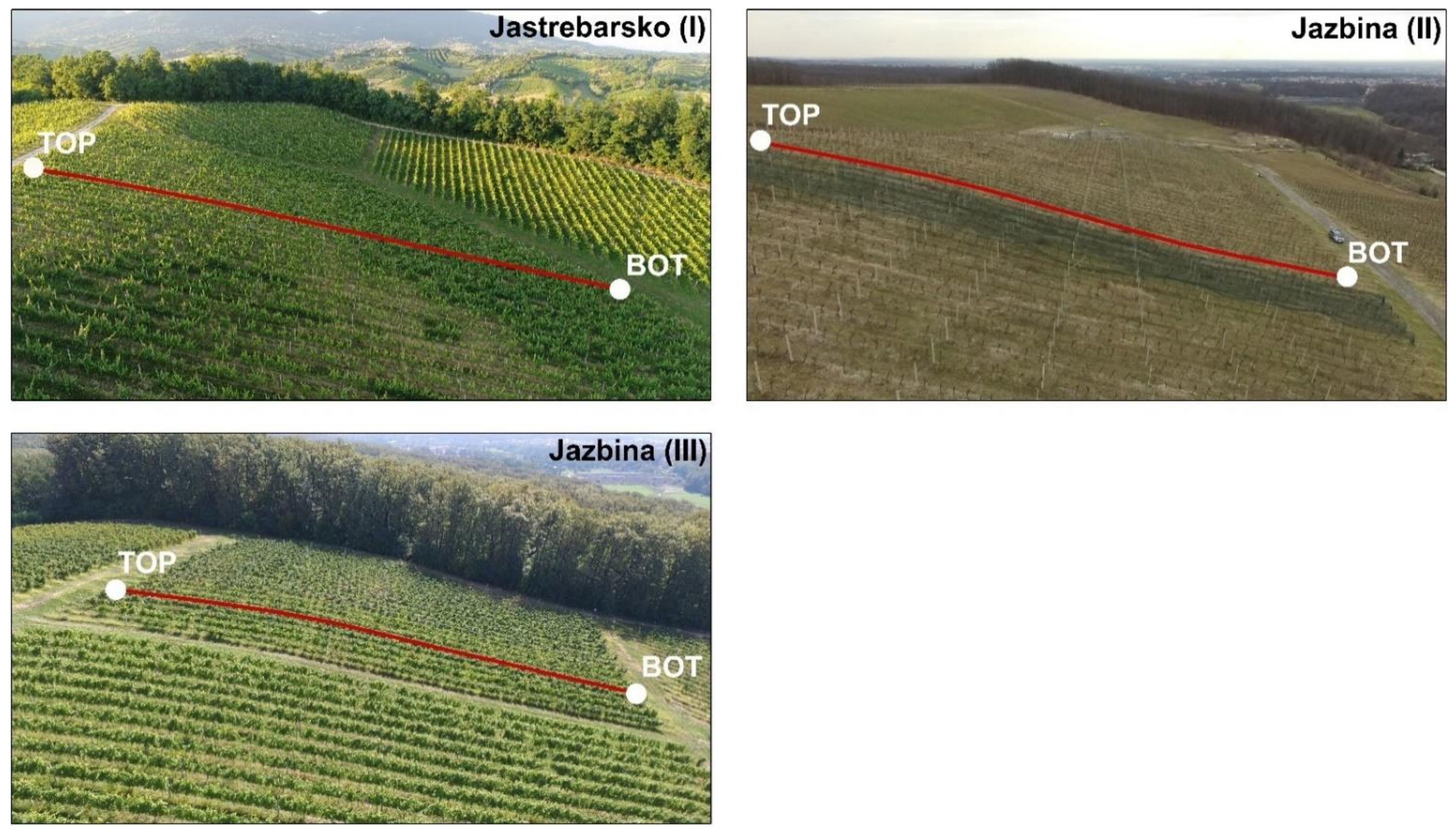
2.1. Experimental Site and Soil Properties

The experimental study was performed in central Croatia (in Zagreb and the nearby southwestern surrounding area). Three selected locations are vineyards located in the same climatic zone (humid continental climate), with the same management practices, i.e., each vineyard is intercropped with grass (2 m wide) parallel with the slope ranging from 10 to 20% (Figure 1). The selected vineyards were Jastrebarsko (45°41′22″ N 15°38′22″ E, noted location I), and two locations in Jazbina (45°51′27.0″ N 16°00′14.4″ E; 45°51′24″ N 16°00′22″ E, noted locations II and III, respectively). The study was performed during 2019 and 2020, focusing on the interrow area, where erosion is the most intense. The samples were collected at the top and the bottom hillslope positions from both the topsoil and the subsoil horizons. Besides the disturbed samples, a triplicate of undisturbed samples was taken as well using soil cores (250 cm3). On each location, soil pits were dug at both hillslope positions, and the soil profiles were described based on the FAO guidelines [47].
According to the WRB classification system [48], all soil profiles were classified into the reference soil group of Stagnosols. These represent the most widespread soils of continental Croatia [49,50]. Although all of the studied soils are classified as Stagnosols, they are not entirely uniform in their properties. Accordingly, principal and/or supplementary WRB qualifiers somewhat vary among the vineyards and between the slope positions (Table 1). The main differences among the analyzed profiles are as follows: (a) profile I-TOP had some shrink-swell cracks and notably more clay (averagely 37.5%) than other profiles (Table 1); (b) due to leaching, profiles II_TOP and III_TOP showed pronounced vertical increase in clay content (Table 1); (c) due to colluviation, at each location the Apg horizon is deeper at the bottom profile than at the top profile (Table 1). All disturbed soil samples were air-dried, crushed, and sieved through a 2 mm sieve. Soil particle size distribution was determined using the pipette method, with wet sieving and sedimentation after dispersion with sodium-pyrophosphate [51]. The soil pH was measured using the Mettler Toledo MPC 227 conductivity/pH-meter in water (pH H2O) (HRN ISO 10390:2005). The organic matter content was determined by sulfochromic oxidation (HRN ISO 14235:1998). The selected soil chemical and physical parameters are presented in Table 1.

2.2. Soil Hydraulic Properties Estimation

SHP were determined on undisturbed soil cores (250 cm3; inner diameter 80 mm and height 50 mm) taken from Apg and Bg/Btg horizons at three vineyards (top and bottom hillslope positions). The soil sampling was performed in three replicates by carefully using a hammer and a sample ring insertion tool, after which soil cores were transported to the laboratory and stored at 4 °C till analysis. SHP were estimated by applying the simplified evaporation method [52] and using the HYPROP (METER Group, Pullman, WA, USA) automatized system [53]. The 18 undisturbed soil sample (250 cm3) were saturated from the bottom of the sample. After the saturation phase was completed, two tensiometers were placed inside the undisturbed soil sample on the HYPROP device at two depths and measured the soil water tension [54]. The evaporation method considers the change in the sample weight and matrix potential (i.e., soil water tension) in the soil sample during the evaporation drying process. It allows accurate characterization of the water-retention properties in the porous media [23]. The measurement is finished when the soil sample evaporates and the tensiometers reach their measurement peak (e.g., air entry point). The results allow the representation of SWRC and SHCC [55].
After the determination of data points for water content, hydraulic conductivity was calculated using the water flow velocity ( q i [cm d−1]) between time points t i 1 and t i through a horizontal plane in the middle of the two tensiometers as explained in Singh et al. [55]:
q i = 1 2 V i / t i A
where V i is the change in water volume in the sample (cm3), t i is the time interval between two consecutive measurement points, and   A is the cross-sectional area (cm2) of the column.
The data points for the hydraulic conductivity function were calculated by inverting Darcy’s equation [55]:
K i h i = q i h i z 1
where h i (cm) is the time- and space-averaged tension, h i is the difference in tensions between the two tensiometers tips, and z (cm) is the distance between the tensiometer. The calculations assume that moisture tension and water content are distributed linearly through the column and, therefore, the arithmetic mean of the tensions at two points was used. This simplified assumption was shown to provide accurate results because linearity errors in fluxes and tensions cancel each other out [56].
After the HYPROP analysis, the undisturbed soil sample was removed from the base sensor and the tensiometers were carefully removed from the holes inside the sample. The next step was the preparation of subsamples for the WP4C device (METER Group, Pullman, WA, USA). The instrument can be combined with HYPROP to measure water potential in the dry range of the soil sample. WP4C is capable of measuring both matric and osmotic potential (applicable for salinity-affected soils) that completes the SWCC [27] and it is used for the water potential measurements in the dry range of the soil sample.

2.3. Fitting of the SWRC and SHCC Using Uni- and Bimodal Hydraulic Models

The hydraulic functions based on the HYPROP and WP4C measurement data were fitted using HYPROP-FIT software (Version 4.2.2.0). Two most commonly applied soil hydraulic models were used and compared: uni- and bimodal porosity models.
In the first approach, fitting was performed using van Genuchten–Mualem (VGM) model [57,58]:
θ h = θ r + θ s θ r 1 + α h n m
S e h = θ h θ r θ s θ r = 1 1 + α h n m
K θ = K s S e l 1 1 S e 1 m   m 2
where h (cm) is pressure head, θ , θ r , and θ s (cm3 cm−3) are the present, residual, and saturated water contents, respectively. Parameter S e represents effective saturation (cm3 cm−3). Parameters α (cm−1), n (unitless) and m (unitless) are the empirical parameters that describe shapes of the SWRC and SHCC, where m = 1 1/n. K is the unsaturated hydraulic conductivity function (cm day1).
In the second approach, a bimodal model [31] was used as well, which can describe a structured soil with developed macropores. Following Durner [31], the porous medium can be divided into i overlapping VGM functions weighted by the factor ω i .
S e = i = 1 k ω i 1 ( 1 + α i h n i m i
with the sum of ω i and ω k being equal to 1. By combining the bimodal retention functions with Mualem’s [58] pore-size distribution model, the bimodal unsaturated hydraulic conductivity can be described with the following equation [59]:
K S e = K s i = 1 k ω i S e i l i = 1 k ω i α i 1 1 S e i 1 m i m i i = 1 k ω i α i 2
Fitting quality for soil hydraulic parameters estimation is given in terms of the root mean square error (RMSE), which indicates the mean distance between the data point and the fitted function:
R M S E = 1 r i = 1 r y i i 2
where yi and ŷi are measured and model-predicted quantities, respectively, i.e., water contents, θ or hydraulic conductivities, log10(K). The model error for water retention (RMSE_θ) was calculated separately from the model error for hydraulic conductivity (RMSE_K).

2.4. Water Flow Modeling

Numerical modeling was performed using the HYDRUS-1D program (version 4.0) [39] that uses the Galerkin-type linear finite element scheme to solve the governing flow equations for uni- and bimodal porosity models. Here, a one-dimensional model was applied for hillslope as the aim was to directly compare top and bottom soil profiles between the three sites (I, II, and III) in terms of uni- and bimodal models and also the soil hydraulic properties responses.
Water flow simulations were based on a numerical solution of the Richards equation for variably-saturated media assuming root water uptake, i.e., grassed interrow strip with the Feddes approach [60] based on the potential uptake parameters according to Wesseling et al. [61]. Richards’ equation is assumed as follows:
θ t = z K h z + 1 S
where t is time (T), z is the spatial coordinate (L), and S is the sink term representing root water uptake (L−1), as stated already above.
Root depth was assumed as 15 cm with maximum root density as the grass cover is well developed and maintained for several growing seasons at all three sites. The simulations were performed for six profiles (three locations at top and bottom positions). The profiles were set down to 110 cm depth with the layering according to Table 1 (Apg/Bg/Btg horizon distribution). An atmospheric boundary condition (precipitation and evapotranspiration) with surface runoff assuming evapotranspiration and rainfall was selected at the soil surface, while free-drainage conditions were imposed at the bottom, at the 110 cm depth, as there was no groundwater table effect at selected plots. The initial condition for water flow was set as a pressure head of −100 cm for all profiles in order to have the same conditions for the comparison of the effects of SHP and layering on water dynamics. The daily evapotranspiration was calculated with the Penman–Monteith equation [62] implemented in the HYDRUS-1D based on the meteorological observations collected at Maksimir, Zagreb meteorological station (https://meteo.hr/ (accessed on 21 July 2021)). The simulations were carried out for a one-year period, i.e., the year 2020, using the one-dimensional soil profile with 101 nodes. Numerical simulations assuming uni- and bimodal SHP modeling approach with HYDRUS code [39] for unsaturated soil zone were applied to quantify and visualize differences in water dynamics among three sites for top and bottom positions in our study.

3. Results and Discussion

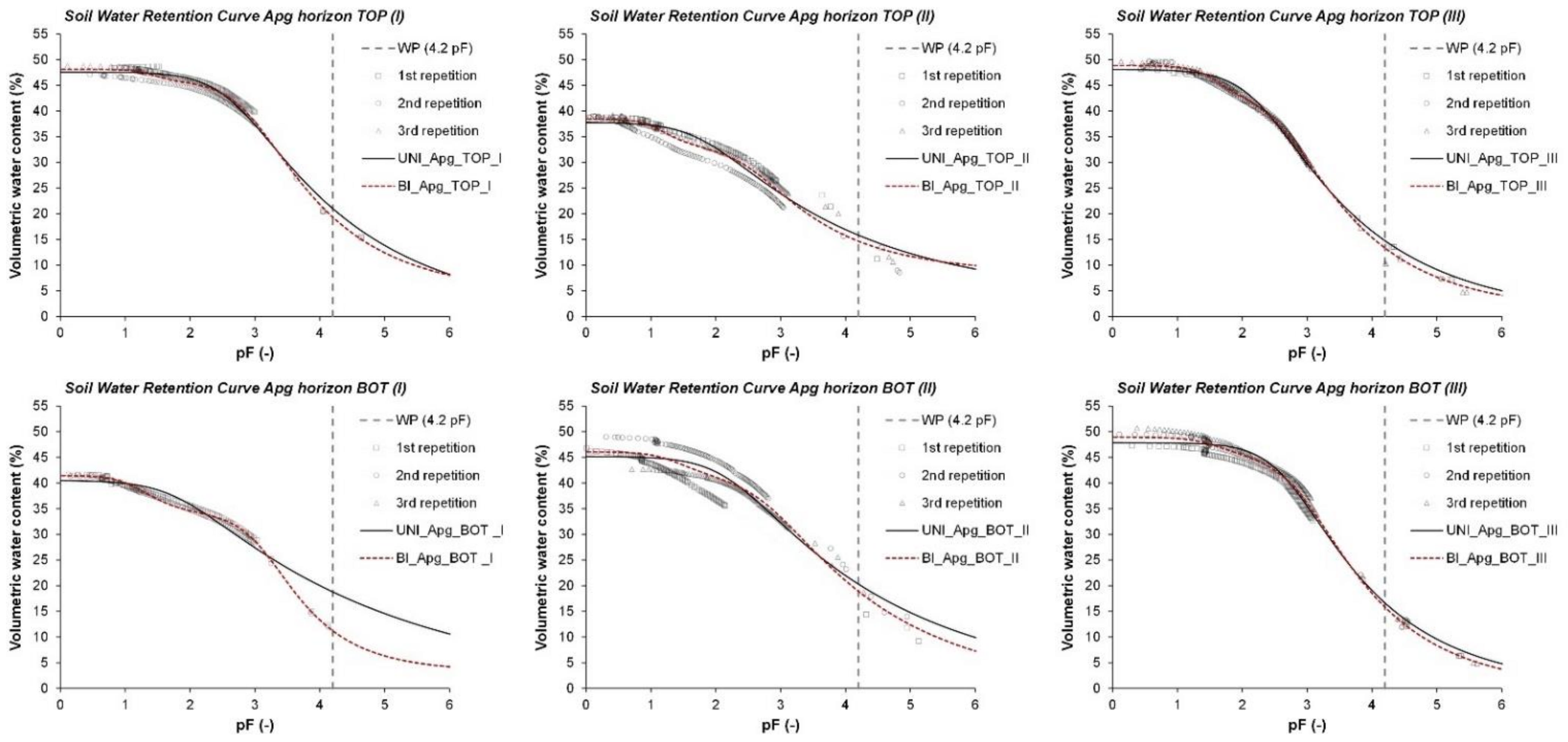
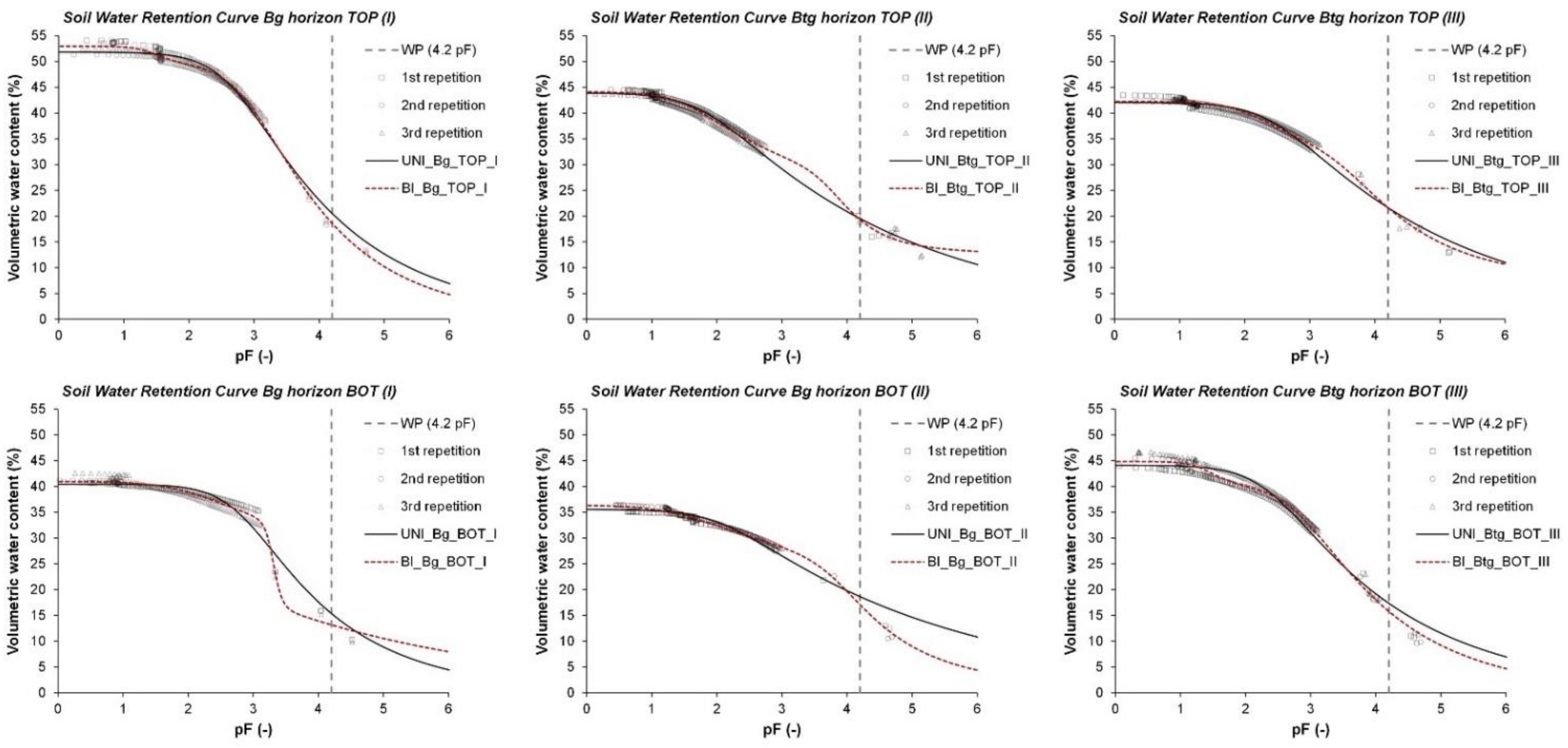
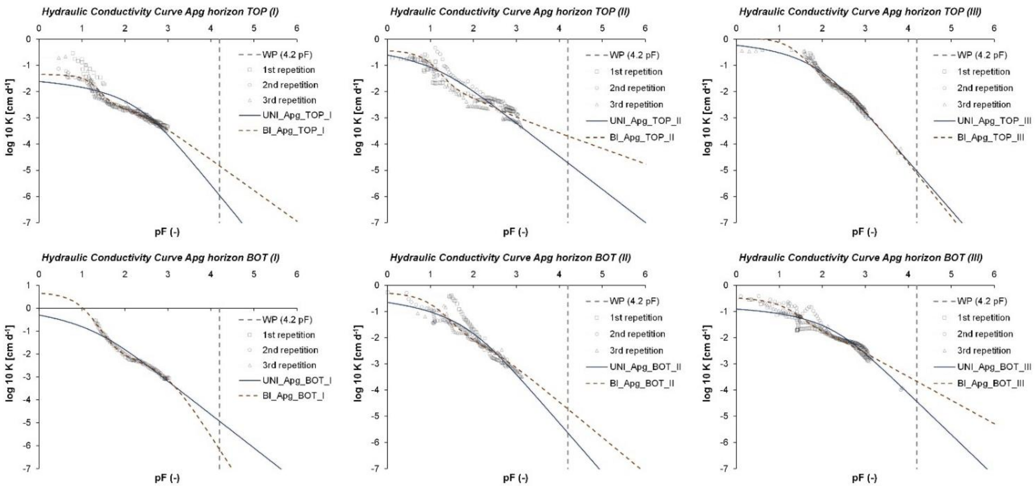
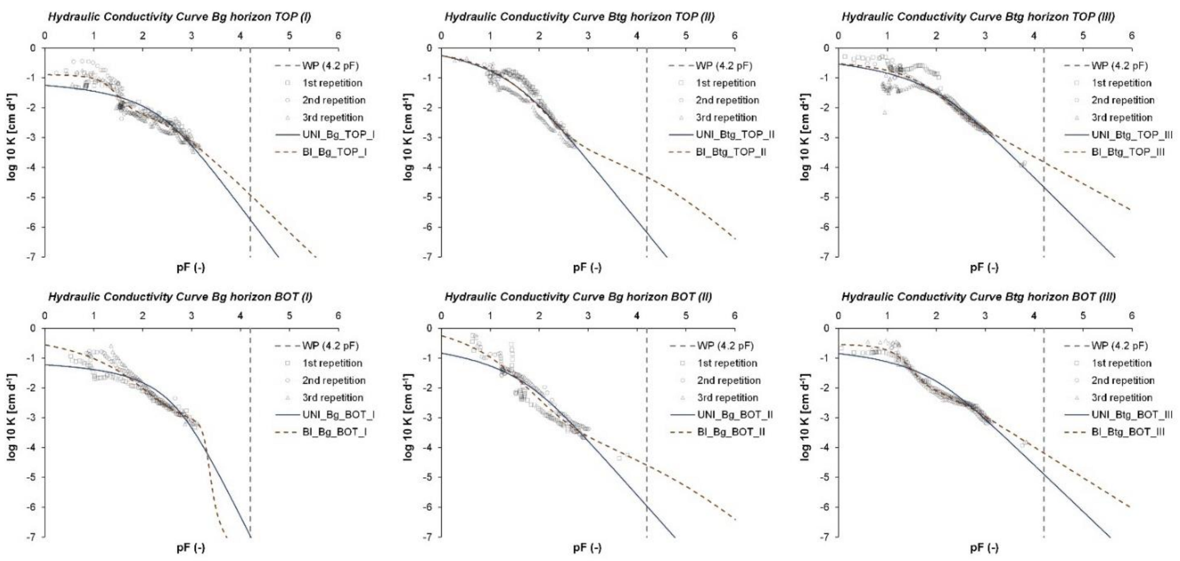
3.1. Soil Hydraulic Properties

The HYPROP-fitted SWRC for the three locations (I, II, and III) using the uni- and bi-modal water retention models for the first Apg (Figure 2), and for the second Bg/Btg horizons (Figure 3), match the measured data points for most samples, depths, and hillslope locations, except on location II at bottom slope position (Apg_BOT_II), where a larger range between data from three replicates was observed for the first horizon. Relatively large differences in θs between Apg and Bg/Btg horizon were estimated at the bottom of location II, although the particle size distribution and organic carbon content were similar. As mentioned above (Figure 2), SWRC for Apg horizon showed a larger data range between three replicates, which indicates the possibility of unreliable hydraulic parameter estimation at this particular location. As the cylinders cover a relatively small area (Ø 80 mm), replicates are necessary, especially in agricultural soils, where it could indicate soil heterogeneity. These differences in replications could be a result of soil erosion which can lead to the soil heterogeneity at the bottom; however, this needs to be further investigated. At location III, θs was largest at the top Apg horizon, which also had the highest porosity/lowest bulk density values, especially compared to the top Btg horizon. Although the top Btg horizon has the largest amount of clay particles, θs was the lowest, which can be caused by the highest bulk density values i.e., the lowest porosity [63], and being connected to the difference in organic carbon content [64]. Even though the data points (Apg_BOT_II) near saturation are more dispersed compared to the other soil horizons, the data at the dry range (around pF 4.2) are more uniform, thus giving validity to the measurements. This indicates the importance of covering the full range of soil water retention curve measurements. The evaporation-based HYPROP method provided a simultaneous fit of the soil water retention and the hydraulic conductivity functions (Figure 4 and Figure 5). As previously reported, the evaporation method provides high-resolution water retention and hydraulic conductivity data [56], highly applicable for the majority of soils [65,66,67].
The van Genuchten model and its bimodal form curves followed the data agreeably; although, we can clearly notice that bimodal performed better in particular cases where nonlinearity in soil hydraulic data was observed (e.g., Figure 2 and Figure 3; Apg_TOP_II; Bg_BOT_II; Btg_BOT_III). In some cases, fitted unimodal SWRC did not follow the dry range data derived from WP4C measurements (e.g., Figure 2 and Figure 3; Apg_BOT_I; Bg_BOT_I; Bg_BOT_II). The same behavior is reproduced at the SHCC curves, which in some cases showed bimodal character (e.g., Figure 4, Apg_TOP_I, Apg_TOP_II, and Btg_BOT_III). The soil water retention dry range data present an important part of the SWRC fitting as it can largely influence its shape and soil water content at pF 4.2, the wilting point, with similar already being documented [27]. Here, we had extended our wet range data using the WP4C to obtain the retention points near the wilting point, and reproduce more reliable results. For even more reliable results of the SHCC, some authors recommended that the evaporation data should be additionally combined with separate conductivity measurements near saturation by using, for example, tension disc infiltrometers [68].
The final SHP and its statistical evaluation (RMSE) derived from the HYPROP-FIT program using uni- and bimodal soil hydraulic models are presented in Table 2 and Table 3. Both uni- and bimodal fits of the soil water retention models resulted in relatively similar values of θs (0.356 to 0.518 cm3 cm−3 for unimodal and 0.364 to 0.529 cm3 cm−3 for bimodal, respectively). Similarly, fitted Ks values ranged from 0.0431 to 2.67 cm day−1 for uni- and from 0.0493 to 5.15 cm day−1 for bimodal models, respectively. These soil properties indicate relatively large water retention capacity and low permeability, thus having the potential for surface runoff generation as they are located on the sloped landscape. As far as for model fitting evaluation, soil water content’s RMSE ranged from 0.0084 to 0.0248 cm3 cm−3 for the uni-model and from 0.0037 to 0.0225 cm3 cm−3 for the bimodal model, respectively. The model fitting for the hydraulic conductivity ranged from 0.1505 to 0.3422 cm day−1 for uni- model and from 0.078 to 0.3632 cm day−1 for the bimodal model, respectively. The RMSE evaluation clearly indicates that both models performed very well in the goodness of fit to observed data. However, particular care should be taken when evaluating SHP and SWRC/SHCC data. In each case, more appropriate soil hydraulic and water flow models should be selected, as selecting less applicable models can further have a significant effect when applying numerical modeling and quantifying hydrological responses [69]. The selection of a less appropriate model, even if the fittings (data vs. model) are similar, can lead to differences in the water balance when simulating longer periods (this is illustrated in Section 3.2). For the undisturbed soil samples collected from multiple irrigated turfgrass plots in southern and central California, Haghverdi et al. [35] reported that the van Genuchten model with five free parameters had RMSE of 0.007 cm3 cm−3, while Van Genuchten bimodal with five free parameters had RMSE of 0.004 cm3 cm−3. It was concluded that the alternative variants (i.e., PDI and bimodal expressions) outperformed the original unimodal expressions.
With the exception of a few horizons (see above), the water retention did not show the effects of multimodal pore size distributions. Since the HYPROP method focuses on the drying SWRC, the SWRC range close to full water saturation was not fully captured, such that the variations in the range of the structural macro-porosity are hardly described here. The bimodality observed with the present method is related to the textural pore size ranges, i.e., non-uniform pore size distributions caused by textural variations [31,70].
For the SWRC as a capacity function, the structural macroporosity is on the one hand not fully in the range of measurement by the HYPROP, and on the other hand, the pore volume fraction occupied by macropores is often relatively small compared to the bulk pore volume [32] and is difficult to detect considering the measurement limitations. However, for the hydraulic conductivity function as an intensity function, the bimodality is more pronounced because the hydraulic conductivity is highly dependent on pore size and pore connectivity and much less on the pore volume [71,72]. Therefore, the SHCC is multimodal for almost all samples, but notably for Apg_TOP_I, Apg_TOP_II, and Btg_BOT_III (Figure 4 and Figure 5).

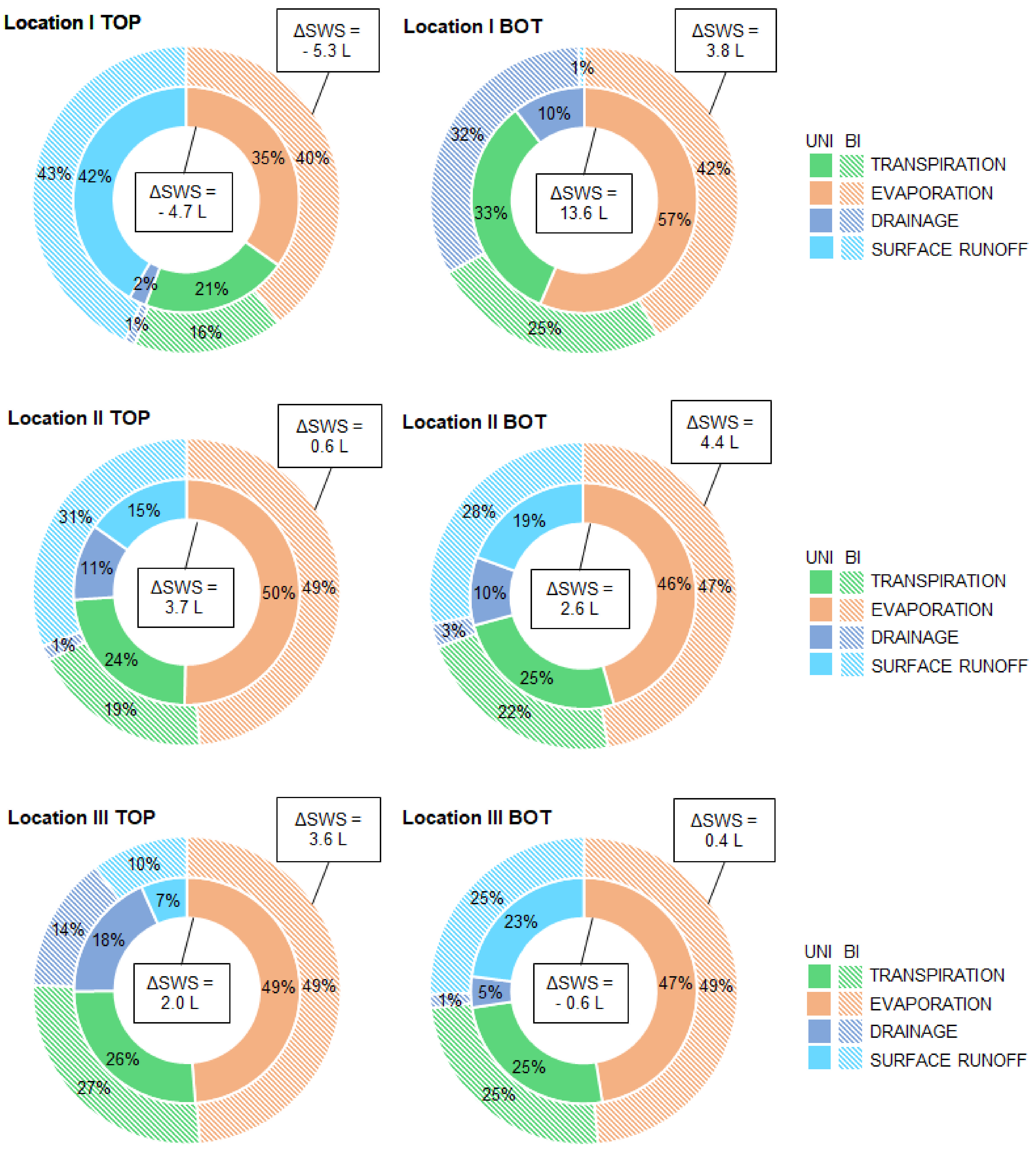
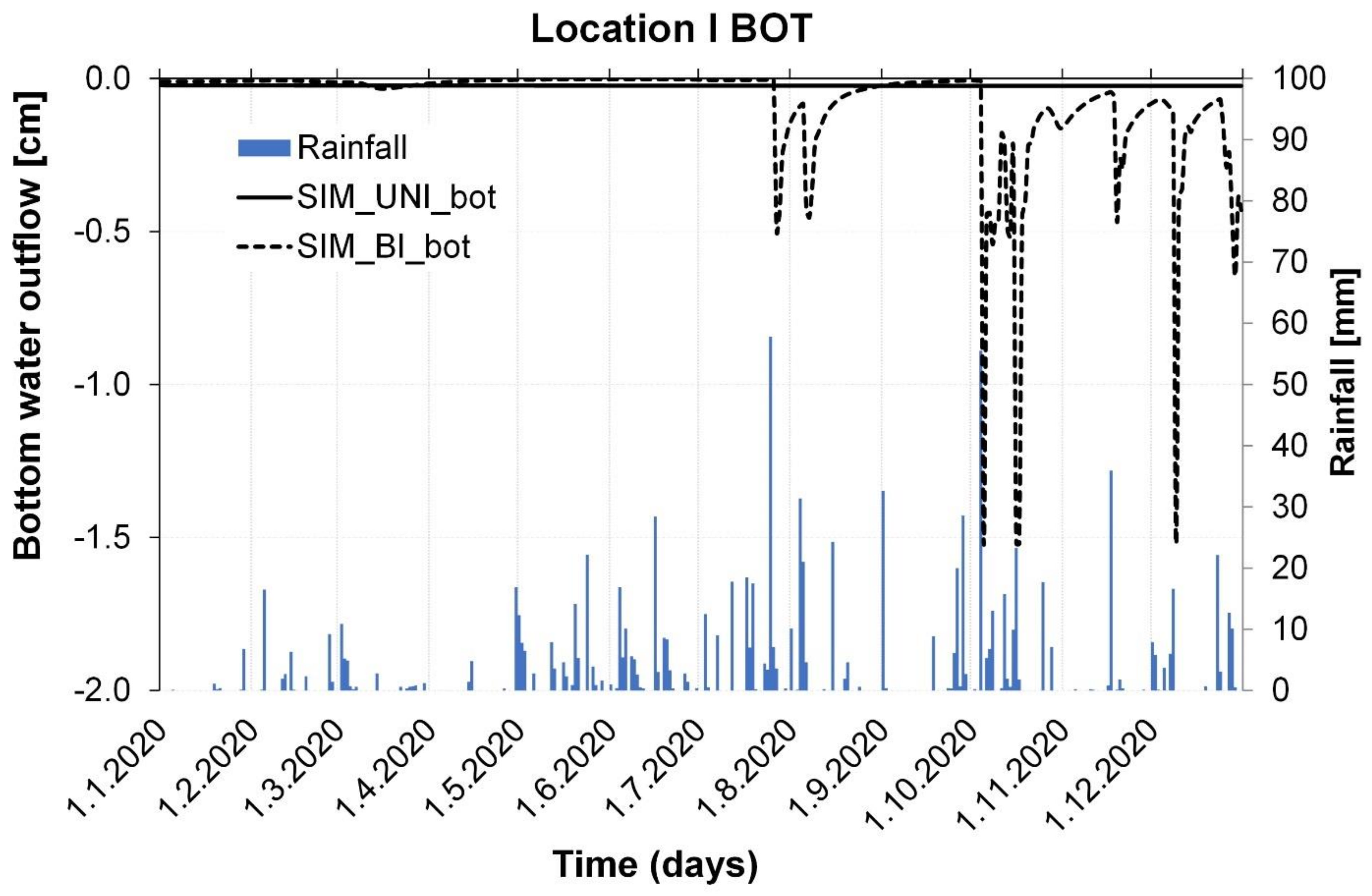
3.2. Water Flow Modeling

With the fitted uni- and bimodal SHP, the soil water balance and the soil water dynamics during a one-year period (2020) were simulated for each profile (TOP vs. BOT) at three locations (Figure 6 and Figure 7) using HYDRUS-1D assuming local equilibrium. The simulations were used to visualize the effect of uni- and bimodal soil hydraulic functions in terms of soil water dynamics in the erosion-affected landscape. The modeling results show an appreciable representation of cumulative flux distribution in profiles, i.e., surface runoff, infiltration, and bottom flux. In general, both models provided similar fluxes distribution at each position between infiltration, surface runoff, and drainage (bottom flux), with a few exceptions mostly connected to the positions where nonlinearity in SHP was noticed (e.g., I_BOT and II_TOP positions). The surface runoff amount is directly connected to the predicted value of the saturated hydraulic conductivity, Ks, which was very low (below 3 cm day−1) in most cases, with the exception of Ks of 5.15 cm day−1 for the bimodal model at the bottom profile at location I. This set of SHP (location I bottom profile) with similar infiltration generated considerably larger bottom flux with the bimodal function (Figure 6). This example will be further discussed below. When comparing the top and bottom positions at each site, for the first two locations (I and II), larger surface runoff is generated at the top position while it is the other way around at the third (III) location). This indicates that local scale SHP was of greater importance and had more relevance as compared to fluxes at the hillslope scale. Details of water balance in Figure 7 further illustrate the similarity of flux components and differences at particular locations (e.g., I_BOT).
Figure 8 shows the daily temporal resolution of a bottom flux at the bottom profile at location I, which indicates the largest nonlinearity and bimodality in water retention data (Figure 2 and Table 3). The simulation using the bimodal SHP predicted a larger and highly dynamic bottom flux (Figure 8) as compared to the unimodal representation. The presented difference supports the discussion related to the importance of appropriate hydraulic model selection. Large bottom flux is also connected to the profile horizon depth where Apg is 88 cm deep; thus, its Ks value of 5.15 cm day−1 is a cause of a large bottom flux in the bimodal approach. This large difference is caused by the shape of the two functions (SWRC, and SHCC), which control the relation between smaller values of the soil water capacity and higher hydraulic conductivities. In the case of the bimodal function during drainage, this leads to increased bottom flux. This example demonstrates the relevance of adequate parameterization of soil hydraulic functions in order to capture the hydrological response of erosion-affected soil systems.
The SHCC estimations via the van Genuchten–Mualem model can result in relatively low performance in the near saturation range due to the inability to account for macropore flow [73,74,75]. Furthermore, Ks is a highly variable soil hydraulic property dependent upon the pore geometry at the scale of interest [74] and seasonal variability [75]. Significant variabilities in Ks estimations might occur when using different estimation procedures [76] and measurement techniques [77], ultimately reflecting on the SHCC estimations. Further studies are needed to determine how adding extra near saturation hydraulic conductivity measurements to HYPROP+WP4C affects the numerical simulation results.
Note that with the present method, the SHP in still unsaturated soil close to full pore water saturation reflecting the effect of the macropores could not be identified with the HYPROP method and relatively small sample size. As reported by Yeh et al. [78], under the same saturated hydraulic conductivity function, the wetting front of the bimodal model moves down faster. This results in changes in the pressure head, water content, and internal stress of the soil. The results show that the water content and suction stress changes in the bimodal model are higher than those of the unimodal model due to the difference in water retention capacity. The present parameter determination and flow modeling still assume local equilibrium conditions in the pressure head of the pore water in the different pore systems. In the case of non-equilibrium-type preferential flow, when infiltrating water bypasses most of the unsaturated soil matrix [32], the kinetics of the capillary-driven macropore–matrix exchange flux needs to be considered, in addition to the bi- or multimodal porosity functions. In this case, the flow modeling requires using a dual-permeability approach with two interacting flow domains, in which the two-pore systems are treated separately, each having separate hydraulic functions. The validity of the increasingly complex modeling approaches, however, needs to be further tested by comparing with field or experimental tracer data, e.g., on soil columns.

4. Conclusions

The study illustrated that erosion-affected soil structural properties governing hillslope hydrology in the arable landscape, in this case, vineyards, were evident and had a significant impact on SHP and, consequently, soil water dynamics. Both unimodal and bimodal soil hydraulic models fitted the data agreeably; although, it can be clearly noticed that the bimodal model performed better in particular cases where data showed non-uniform pore size distributions. HYDRUS-1D simulations showed, in general, that both models provided a similar distribution of flux components between infiltration, surface runoff, and drainage (bottom flux) in most cases. Overall, the differences generated when using the bimodal hydraulic functions can lead to a large discrepancy in water flow quantification. Location I bottom profile simulation revealed the influence of the shape of two functions (SWRC, and SHCC), which control the relation between soil water capacity and hydraulic conductivities in the case of bimodal function during drainage, leading to increased bottom flux. It is evident that the SHP and water dynamics in highly erosion-affected heterogeneous soils with developed structure and pore space (e.g., compacted soil with cracks and biopores) cannot be adequately explained using the unimodal porosity functions or by applying single porosity models. However, the validity of more complex approaches should be further tested and parametrization should be performed with extra care, as using the non-appropriate model can lead to errors in the water balance. The study indicates that local scale SHP were of more considerable importance and had more relevance as compared to fluxes at the hillslope scale, and that an accurate parameterization of SHP is required to capture the hydropedological response of erosion-affected soil systems.

Author Contributions

Conceptualization, V.F., J.D., V.K., and L.F.; methodology, V.F., J.D., V.K., G.O., F.K., I.M. (Ivan Magdić), V.R., S.S., I.M. (Ivan Mustać), M.B.K., H.H., A.H., H.H.G., and L.F.; software, V.F., J.D., V.K., I.M. (Ivan Magdić), and H.H.G.; validation, V.F., J.D., V.K., I.M. (Ivan Magdić), H.H., A.H., H.H.G., and L.F.; formal analysis, V.F., J.D., V.K., G.O., F.K., I.M. (Ivan Magdić), V.R., S.S., I.M. (Ivan Mustać), M.B.K., H.H., A.H., H.H.G., and L.F.; investigation, V.F., J.D., V.K., F.K., I.M. (Ivan Magdić), I.M. (Ivan Mustać), and L.F.; data curation, V.F., J.D., V.K., F.K., I.M. (Ivan Magdić), I.M. (Ivan Mustać), and M.B.K.; writing—original draft preparation, V.F., J.D., and V.K.; writing—review and editing, G.O., V.R., S.S., H.H., A.H., H.H.G., and L.F.; visualization, V.F.,V.K., and H.H.G.; supervision, V.F.; funding acquisition, V.F. and G.O. All authors have read and agreed to the published version of the manuscript.

Funding

This research was funded by Croatian Science Foundation, grant number UIP-2019-04-5409, project: “Subsurface preferential transport processes in agricultural hillslope soils—SUPREHILL”. The APC was funded by University of Zagreb Faculty of Agriculture.

Institutional Review Board Statement

Not applicable.

Informed Consent Statement

Not applicable.

Data Availability Statement

Data available on demand.

Acknowledgments

We are thankful to the technical staff who provided support during our field experiments. We acknowledge the historical data availability and sharing on those sites provided by the Department of Soil Science and the Department of Viticulture and Enology, Faculty of Agriculture Zagreb, and Mladina plus d.o.o. company.

Conflicts of Interest

The authors declare no conflict of interest.

References

  1. Poesen, J. Soil erosion in the Anthropocene: Research needs. Earth Surf. Process. Landforms 2018, 43, 64–84. [Google Scholar] [CrossRef]
  2. Borrelli, P.; Alewell, C.; Alvarez, P.; Anache, J.A.A.; Baartman, J.; Ballabio, C.; Bezak, N.; Biddoccu, M.; Cerdà, A.; Chalise, D.; et al. Soil erosion modelling: A global review and statistical analysis. Sci. Total Environ. 2021, 780, 146494. [Google Scholar] [CrossRef] [PubMed]
  3. Oldeman, L.R. Global extent of soil degradation. In Soil Resilience and Sustainable Landuse; Greenland, D.J., Szabolcs, I., Eds.; CAB International: Wallingford, UK, 1994; pp. 99–119. [Google Scholar]
  4. Wuepper, D.; Borrelli, P.; Finger, R. Countries and the global rate of soil erosion. Nat. Sustain. 2020, 3, 51–55. [Google Scholar] [CrossRef]
  5. Govers, G.; Quine, T.A.; Desmet, P.J.J.; Walling, D.E. The relative contribution of soil tillage and overland flow erosion to soil redistribution on agricultural land. Earth Surf. Process. Landforms 1996, 21, 929–946. [Google Scholar] [CrossRef]
  6. Comino, J.R.; Senciales, J.M.; Ramos, M.C.; Martinez-Casasnovas, J.A.; Lasanta, T.; Brevik, E.C.; Ries, J.B.; Sinoga, J.D.R. Understanding soil erosion processes in Mediterranean sloping vineyards (Montes de Málaga, Spain). Geoderma 2017, 296, 47–59. [Google Scholar] [CrossRef] [Green Version]
  7. Casalí, J.; Giménez, R.; De Santisteban, L.; Álvarez-Mozos, J.; Mena, J.; Lersundi, J.D.V.d. Determination of long-term erosion rates in vineyards of Navarre (Spain) using botanical benchmarks. CATENA 2009, 78, 12–19. [Google Scholar] [CrossRef]
  8. Biddoccu, M.; Ferraris, S.; Opsi, F.; Cavallo, E. Long-term monitoring of soil management effects on runoff and soil erosion in sloping vineyards in Alto Monferrato (North–West Italy). Soil Tillage Res. 2016, 155, 176–189. [Google Scholar] [CrossRef]
  9. Paroissien, J.-B.; Lagacherie, P.; Le Bissonnais, Y. A regional-scale study of multi-decennial erosion of vineyard fields using vine-stock unearthing–burying measurements. Catena 2010, 82, 159–168. [Google Scholar] [CrossRef]
  10. Prosdocimi, M.; Cerdà, A.; Tarolli, P. Soil water erosion on Mediterranean vineyards: A review. Catena 2016, 141, 1–21. [Google Scholar] [CrossRef]
  11. Verheijen, F.G.A.; Jones, R.J.A.; Rickson, R.J.; Smith, C.J. Tolerable versus actual soil erosion rates in Europe. Earth Sci. Rev. 2009, 94, 23–38. [Google Scholar] [CrossRef] [Green Version]
  12. Novara, A.; Pisciotta, A.; Minacapilli, M.; Maltese, A.; Capodici, F.; Cerdà, A.; Gristina, L. The impact of soil erosion on soil fertility and vine vigor. A multidisciplinary approach based on field, laboratory and remote sensing approaches. Sci. Total Environ. 2018, 622, 474–480. [Google Scholar] [CrossRef] [PubMed] [Green Version]
  13. Rodrigo-Comino, J.; Senciales, J.M.; Sillero-Medina, J.A.; Gyasi-Agyei, Y.; Ruiz-Sinoga, J.D.; Ries, J.B. Analysis of Weather-Type-Induced Soil Erosion in Cultivated and Poorly Managed Abandoned Sloping Vineyards in the Axarquía Region (Málaga, Spain). Air Soil Water Res. 2019, 12, 117862211983940. [Google Scholar] [CrossRef]
  14. Bogunovic, I.; Telak, L.J.; Pereira, P. Experimental Comparison of Runoff Generation and Initial Soil Erosion Between Vineyards and Croplands of Eastern Croatia: A Case Study. Air Soil Water Res. 2020, 13, 117862212092832. [Google Scholar] [CrossRef]
  15. Cerdan, O.; Govers, G.; Le Bissonnais, Y.; Van Oost, K.; Poesen, J.; Saby, N.; Gobin, A.; Vacca, A.; Quinton, J.; Auerswald, K.; et al. Rates and spatial variations of soil erosion in Europe: A study based on erosion plot data. Geomorphology 2010, 122, 167–177. [Google Scholar] [CrossRef]
  16. Groh, J. Crop growth and soil water fluxes at erosion-affected arable sites: A model inter-comparison based on weighing-lysimeter observations. In Proceedings of the EGU General Assembly Conference Abstracts, Vienna, Austria, 3–8 May 2020. [Google Scholar]
  17. Van Oost, K.; Van Muysen, W.; Govers, G.; Heckrath, G.; Quine, T.A.; Poesen, J. Simulation of the redistribution of soil by tillage on complex topographies. Eur. J. Soil Sci. 2003, 54, 63–76. [Google Scholar] [CrossRef]
  18. Horn, R.; Smucker, A. Structure formation and its consequences for gas and water transport in unsaturated arable and forest soils. Soil Tillage Res. 2005, 82, 5–14. [Google Scholar] [CrossRef]
  19. Rieckh, H.; Gerke, H.H.; Siemens, J.; Sommer, M. Water and Dissolved Carbon Fluxes in an Eroding Soil Landscape Depending on Terrain Position. Vadose Zone J. 2014, 13, vzj2013–10. [Google Scholar] [CrossRef]
  20. Herbrich, M.; Gerke, H.H.; Bens, O.; Sommer, M. Water balance and leaching of dissolved organic and inorganic carbon of eroded Luvisols using high precision weighing lysimeters. Soil Tillage Res. 2017, 165, 144–160. [Google Scholar] [CrossRef]
  21. Deumlich, D.; Schmidt, R.; Sommer, M. A multiscale soil-landform relationship in the glacial-drift area based on digital terrain analysis and soil attributes. J. Plant Nutr. Soil Sci. 2010, 173, 843–851. [Google Scholar] [CrossRef]
  22. Filipović, V.; Gerke, H.H.; Filipović, L.; Sommer, M. Quantifying Subsurface Lateral Flow along Sloping Horizon Boundaries in Soil Profiles of a Hummocky Ground Moraine. Vadose Zone J. 2018, 17, 170106. [Google Scholar] [CrossRef] [Green Version]
  23. Schindler, U.; von Unold, G.; Durner, W.; Mueller, L. Recent Progress in Measuring Soil Hydraulic Properties. In Proceedings of the International Academy of Engineers (IA-E), Pattaya, Thailand, 24–25 April 2015; pp. 24–25. [Google Scholar]
  24. Campbell, C.S.; Cobos, D.R.; Rivera, L.D.; Dunne, K.M.; Campbell, G.S. Constructing fast, accurate soil water characteristic curves by combining the wind/schindler and vapor pressure techniques. In Unsaturated Soils: Research and Applications; Springer: Berlin/Heidelberg, Germany, 2012; pp. 55–62. [Google Scholar]
  25. Schaap, M.G.; Leij, F.J.; van Genuchten, M.T. Rosetta: A computer program for estimating soil hydraulic parameters with hierarchical pedotransfer functions. J. Hydrol. 2001, 251, 163–176. [Google Scholar] [CrossRef]
  26. Van Genuchten, M.T.; Simunek, J.; Schaap, M.G.; Skaggs, T.H. Unsaturated Zone Parameter Estimation Using the HYDRUS and Rosetta Software Packages. Proceedings of International Workshop “Uncertainty, Sensitivity, and Parameter Estimation for Multimedia Environmental Modeling”, Rockville, MD, USA, 19–21 August 2003. [Google Scholar]
  27. Shokrana, M.S.B.; Ghane, E. Measurement of soil water characteristic curve using HYPROP2. MethodsX 2020, 7, 100840. [Google Scholar] [CrossRef] [PubMed]
  28. Kodešová, R.; Šimůnek, J.; Nikodem, A.; Jirků, V. Estimation of the Dual-Permeability Model Parameters using Tension Disk Infiltrometer and Guelph Permeameter. Vadose Zone J. 2010, 9, 213–225. [Google Scholar] [CrossRef]
  29. Filipović, V.; Coquet, Y.; Gerke, H.H. Representation of Plot-Scale Soil Heterogeneity in Dual-Domain Effective Flow and Transport Models with Mass Exchange. Vadose Zone J. 2019, 18, 1–14. [Google Scholar] [CrossRef] [Green Version]
  30. Filipović, V.; Defterdarović, J.; Šimůnek, J.; Filipović, L.; Ondrašek, G.; Romić, D.; Bogunović, I.; Mustać, I.; Ćurić, J.; Kodešová, R. Estimation of vineyard soil structure and preferential flow using dye tracer, X-ray tomography, and numerical simulations. Geoderma 2020, 380, 114699. [Google Scholar] [CrossRef]
  31. Durner, W. Hydraulic conductivity estimation for soils with heterogeneous pore structure. Water Resour. Res. 1994, 30, 211–223. [Google Scholar] [CrossRef]
  32. Gerke, H.H. Preferential flow descriptions for structured soils. J. Plant Nutr. Soil Sci. 2006, 169, 382–400. [Google Scholar] [CrossRef]
  33. Jarvis, N.J. A review of non-equilibrium water flow and solute transport in soil macropores: principles, controlling factors and consequences for water quality. Eur. J. Soil Sci. 2007, 58, 523–546. [Google Scholar] [CrossRef]
  34. Gerke, H.H.; van Genuchten, M.T. A dual-porosity model for simulating the preferential movement of water and solutes in structured porous media. Water Resour. Res. 1993, 29, 305–319. [Google Scholar] [CrossRef]
  35. Haghverdi, A.; Najarchi, M.; Öztürk, H.S.; Durner, W. Studying Unimodal, Bimodal, PDI and Bimodal-PDI Variants of Multiple Soil Water Retention Models: I. Direct Model Fit Using the Extended Evaporation and Dewpoint Methods. Water 2020, 12, 900. [Google Scholar] [CrossRef] [Green Version]
  36. Flanagan, D.C.; Gilley, J.E.; Franti, T.G. Water erosion prediction project (WEPP): Development history, model capabilities, and future enhancements. Trans. ASABE 2007, 50, 1603–1612. [Google Scholar] [CrossRef]
  37. Arnold, J.G.; Moriasi, D.N.; Gassman, P.W.; Abbaspour, K.C.; White, M.J.; Srinivasan, R.; Santhi, C.; Harmel, R.D.; Van Griensven, A.; Van Liew, M.W.; et al. SWAT: Model use, calibration and validation. Trans. ASABE 2012, 55, 1491–1508. [Google Scholar] [CrossRef]
  38. Nyakatawa, E.Z.; Reddy, K.C.; Lemunyon, J.L. Predicting soil erosion in conservation tillage cotton production systems using the revised universal soil loss equation (RUSLE). Soil Tillage Res. 2001, 57, 213–224. [Google Scholar] [CrossRef]
  39. Šimůnek, J.; van Genuchten, M.T.; Šejna, M. Recent Developments and Applications of the HYDRUS Computer Software Packages. Vadose Zone J. 2016, 15. [Google Scholar] [CrossRef] [Green Version]
  40. Dettmann, U.; Bechtold, M.; Frahm, E.; Tiemeyer, B. On the applicability of unimodal and bimodal van Genuchten-Mualem based models to peat and other organic soils under evaporation conditions. J. Hydrol. 2014, 515, 103–115. [Google Scholar] [CrossRef] [Green Version]
  41. Rieckh, H.; Gerke, H.H.; Sommer, M. Hydraulic properties of characteristic horizons depending on relief position and structure in a hummocky glacial soil landscape. Soil Tillage Res. 2012, 125, 123–131. [Google Scholar] [CrossRef]
  42. Jakšík, O.; Kodešová, R.; Kubiš, A.; Stehlíková, I.; Drábek, O.; Kapička, A. Soil aggregate stability within morphologically diverse areas. Catena 2015, 127, 287–299. [Google Scholar] [CrossRef]
  43. Nikodem, A.; Kodešová, R.; Fér, M.; Klement, A. Using scaling factors for characterizing spatial and temporal variability of soil hydraulic properties of topsoils in areas heavily affected by soil erosion. J. Hydrol. 2021, 593, 125897. [Google Scholar] [CrossRef]
  44. Bogunovic, I.; Pereira, P.; Kisic, I.; Sajko, K.; Sraka, M. Tillage management impacts on soil compaction, erosion and crop yield in Stagnosols (Croatia). Catena 2018, 160, 376–384. [Google Scholar] [CrossRef]
  45. Haghverdi, A.; Öztürk, H.S.; Durner, W. Studying Unimodal, Bimodal, PDI and Bimodal-PDI Variants of Multiple Soil Water Retention Models: II. Evaluation of Parametric Pedotransfer Functions Against Direct Fits. Water 2020, 12, 896. [Google Scholar] [CrossRef] [Green Version]
  46. Lin, H.; Bouma, J.; Pachepsky, Y.; Western, A.; Thompson, J.; van Genuchten, R.; Vogel, H.-J.; Lilly, A. Hydropedology: Synergistic integration of pedology and hydrology. Water Resour. Res. 2006, 42, W05301. [Google Scholar] [CrossRef]
  47. Jahn, R.; Blume, H.P.; Asio, V.B.; Spaargaren, O.; Schad, P. Guidelines for Soil Description, 4th ed.; FAO: Rome, Italy, 2006. [Google Scholar]
  48. WRB-IUSS. World Reference Base for Soil Resources. World Soil Resources Reports 106; FAO: Rome, Italy, 2014; ISBN 9789251083697. [Google Scholar]
  49. Bogunović, M.; Vidaček, Ž.; Husnjak, S.; Sraka, M. Inventory of soils in Croatia. Agric. Conspec. Sci. 1998, 63, 105–112. [Google Scholar]
  50. Rubinić, V.; Lazarević, B.; Husnjak, S.; Durn, G. Climate and relief influence on particle size distribution and chemical properties of Pseudogley soils in Croatia. Catena 2015, 127, 340–348. [Google Scholar] [CrossRef]
  51. Gee, G.W.; Or, D. Methods of soil analysis: Particle-size analysis. In Methods of Soil Analysis; Dane, J.H., Topp, G.C., Eds.; Soils Science Society of America: Madison, WI, USA, 2002; pp. 1381–1402. [Google Scholar]
  52. Schindler, U.G.; Müller, L. Soil hydraulic functions of international soils measured with the Extended Evaporation Method (EEM) and the HYPROP device. Open Data J. Agric. Res. 2017, 3, 1–7. [Google Scholar] [CrossRef] [Green Version]
  53. Haghverdi, A.; Öztürk, H.S.; Durner, W. Measurement and estimation of the soil water retention curve using the evaporation method and the pseudo continuous pedotransfer function. J. Hydrol. 2018, 563, 251–259. [Google Scholar] [CrossRef]
  54. UMS Manual HYPROP. Version 2015_01. UMS GmbH, Gmunder Straße 37, Munich, Germany. Available online: http://library.metergroup.com/Manuals/UMS/Hyprop_Manual.pdf (accessed on 18 February 2021).
  55. Singh, A.; Haghverdi, A.; Öztürk, H.S.; Durner, W. Developing Pseudo Continuous Pedotransfer Functions for International Soils Measured with the Evaporation Method and the HYPROP System: II. The Soil Hydraulic Conductivity Curve. Water 2021, 13, 878. [Google Scholar] [CrossRef]
  56. Peters, A.; Iden, S.C.; Durner, W. Revisiting the simplified evaporation method: Identification of hydraulic functions considering vapor, film and corner flow. J. Hydrol. 2015, 527, 531–542. [Google Scholar] [CrossRef]
  57. van Genuchten, M.T. A closed-form equation for predicting the hydraulic conductivity of unsaturated soils. Soil Sci. Soc. Am. J. 1980, 44, 892–898. [Google Scholar] [CrossRef] [Green Version]
  58. Mualem, Y. A New Model for Predicting the Hydraulic Conductivity of Unsaturated Porous Media. Water Resour. Res. 1976, 12, 513–522. [Google Scholar] [CrossRef] [Green Version]
  59. Priesack, E.; Durner, W. Closed-Form Expression for the Multimodal Unsaturated Conductivity Function. Vadose Zone J. 2006, 5, 121–124. [Google Scholar] [CrossRef]
  60. Feddes, R.A.; Kowalik, P.J.; Zaradny, H. Simulation of field water use and crop yield. In Simulation Monographs; Wageningen Centre for Agricultural Publishing and Documentation: Wageningen, The Netherlands, 1978. [Google Scholar]
  61. Wesseling, J.G.; Elbers, J.A.; Kabat, P.; Van Den Broek, B.J. SWATRE: Instructions for Input Internal Note; Winand Staring Ctr.: Wageningen, The Netherlands, 1991. [Google Scholar]
  62. Monteith, J.L. Evaporation and surface temperature. Q. J. R. Meteorol. Soc. 1981, 107, 1–27. [Google Scholar] [CrossRef]
  63. Eden, M.; Gerke, H.H.; Houot, S. Organic waste recycling in agriculture and related effects on soil water retention and plant available water: a review. Agron. Sustain. Dev. 2017, 37, 11. [Google Scholar] [CrossRef] [Green Version]
  64. Wesseling, J.G.; Stoof, C.R.; Ritsema, C.J.; Oostindie, K.; Dekker, L.W. The effect of soil texture and organic amendment on the hydrological behaviour of coarse-textured soils. Soil Use Manag. 2009, 25. [Google Scholar] [CrossRef]
  65. Schwen, A.; Zimmermann, M.; Bodner, G. Vertical variations of soil hydraulic properties within two soil profiles and its relevance for soil water simulations. J. Hydrol. 2014, 516, 169–181. [Google Scholar] [CrossRef]
  66. Herbrich, M.; Gerke, H.H. Scales of Water Retention Dynamics Observed in Eroded Luvisols from an Arable Postglacial Soil Landscape. Vadose Zone J. 2017, 16. [Google Scholar] [CrossRef]
  67. Schindler, U.; Mueller, L.; da Veiga, M.; Zhang, Y.; Schlindwein, S.; Hu, C. Comparison of water-retention functions obtained from the extended evaporation method and the standard methods sand/kaolin boxes and pressure plate extractor. J. Plant Nutr. Soil Sci. 2012, 175, 527–534. [Google Scholar] [CrossRef]
  68. Weninger, T.; Bodner, G.; Kreiselmeier, J.; Chandrasekhar, P.; Julich, S.; Feger, K.-H.; Schwärzel, K.; Schwen, A. Combination of Measurement Methods for a Wide-Range Description of Hydraulic Soil Properties. Water 2018, 10, 1021. [Google Scholar] [CrossRef] [Green Version]
  69. Šimůnek, J.; Jarvis, N.J.; van Genuchten, M.T.; Gärdenäs, A. Review and comparison of models for describing non-equilibrium and preferential flow and transport in the vadose zone. J. Hydrol. 2003, 272, 14–35. [Google Scholar] [CrossRef]
  70. Jensen, J.L.; Schjønning, P.; Watts, C.W.; Christensen, B.T.; Munkholm, L.J. Soil Water Retention: Uni-Modal Models of Pore-Size Distribution Neglect Impacts of Soil Management. Soil Sci. Soc. Am. J. 2019, 83, 18–26. [Google Scholar] [CrossRef] [Green Version]
  71. Beck-Broichsitter, S.; Fleige, H.; Dusek, J.; Gerke, H.H. Anisotropy of unsaturated hydraulic properties of compacted mineral capping systems seven years after construction. Soil Tillage Res. 2020, 204. [Google Scholar] [CrossRef]
  72. Beck-Broichsitter, S.; Gerke, H.H.; Leue, M.; von Jeetze, P.J.; Horn, R. Anisotropy of unsaturated soil hydraulic properties of eroded Luvisol after conversion to hayfield comparing alfalfa and grass plots. Soil Tillage Res. 2020, 198, 104553. [Google Scholar] [CrossRef]
  73. Weynants, M.; Vereecken, H.; Javaux, M. Revisiting Vereecken Pedotransfer Functions: Introducing a Closed-Form Hydraulic Model. Vadose Zone J. 2009, 8, 86–95. [Google Scholar] [CrossRef] [Green Version]
  74. Niemann, W.L.; Rovey, C.W., II. A systematic field-based testing program of hydraulic conductivity and dispersivity over a range in scale. Hydrogeol. J. 2009, 17, 307–320. [Google Scholar] [CrossRef]
  75. Bormann, H.; Klaassen, K. Seasonal and land use dependent variability of soil hydraulic and soil hydrological properties of two Northern German soils. Geoderma 2008, 145, 295–302. [Google Scholar] [CrossRef]
  76. Baroni, G.; Facchi, A.; Gandolfi, C.; Ortuani, B.; Horeschi, D.; van Dam, J.C. Uncertainty in the determination of soil hydraulic parameters and its influence on the performance of two hydrological models of different complexity. Hydrol. Earth Syst. Sci. 2010, 14, 251–270. [Google Scholar] [CrossRef] [Green Version]
  77. Fodor, N.; Sándor, R.; Orfanus, T.; Lichner, L.; Rajkai, K. Evaluation method dependency of measured saturated hydraulic conductivity. Geoderma 2011, 165, 60–68. [Google Scholar] [CrossRef]
  78. Yeh, H.-F.; Huang, T.-T.; Lee, J.-W. Effect of Unimodal and Bimodal Soil Hydraulic Properties on Slope Stability Analysis. Water 2021, 13, 1674. [Google Scholar] [CrossRef]
Figure 1. Aerial imagery of three studied vineyards, i.e., Jastrebarsko (I), and two at Jazbina location (II and III), with the indication of hydropedological study location at the top (TOP) and the bottom (BOT) of the slope.
Agronomy 12 00033 g001
Figure 2. Soil water retention curves (SWRC) of the Apg soil horizons at three selected vineyards, i.e., Jastrebarsko (I), Jazbina (II), and Jazbina (III) for top (TOP) and bottom (BOT) positions on the slope using uni- (UNI) and bimodal (BI) soil hydraulic models.
Agronomy 12 00033 g002
Figure 3. Soil water retention curves (SWRC) of the Bg/Btg soil horizons at three selected vineyards, i.e., Jastrebarsko (I), Jazbina (II), and Jazbina (III) for top (TOP) and bottom (BOT) positions on the slope using uni- (UNI) and bimodal (BI) soil hydraulic models.
Agronomy 12 00033 g003
Figure 4. Soil Hydraulic conductivity curves (SHCC) of the Apg soil horizons at three selected vineyards, i.e., Jastrebarsko (I), Jazbina (II), and Jazbina (III) for top (TOP) and bottom (BOT) positions on the slope using uni- (UNI) and bimodal (BI) soil hydraulic models.
Agronomy 12 00033 g004
Figure 5. Soil Hydraulic conductivity curves (SHCC) of the Bg/Btg soil horizons at three selected vineyards, i.e., Jastrebarsko (I), Jazbina (II), and Jazbina (III) for top (TOP) and bottom (BOT) positions on the slope using uni- (UNI) and bimodal (BI) soil hydraulic models.
Agronomy 12 00033 g005
Figure 6. One-year (2020) water flow simulation (HYDRUS-1D) using uni- (UNI) and bimodal (BI) soil hydraulic models at three selected vineyards, i.e., Jastrebarsko (I), Jazbina (II), and Jazbina (III) for top (TOP) and bottom (BOT) positions on the slope. The figure reveals cumulative bottom flux (_bott), infiltration (_inf), and surface runoff (_runoff).
Agronomy 12 00033 g006
Figure 7. Water balance components: transpiration, evaporation, drainage (bottom flux), surface runoff, and soil water storage change (ΔSWS), for uni- (UNI) and bimodal (BI) soil hydraulic models of a one-year simulation (2020) using HYDRUS-1D at three selected vineyards, i.e., Jastrebarsko (I), Jazbina (II) and Jazbina (III), for top (TOP), and bottom (BOT) positions on the slope.
Agronomy 12 00033 g007
Figure 8. Comparison of water flow simulation (HYDRUS-1D) using uni- (UNI) and bimodal (BI) soil hydraulic models at Jastrebarsko (I) bottom (BOT) position during 2020.
Agronomy 12 00033 g008
Table 1. Selected soil properties, i.e., pH (H2O), organic carbon content (%), particle size distribution (%), bulk density (g cm−3), and porosity (%), presented with horizon designation.
Sample NameLocationSoil ProfileDepth (cm)pH
(H2O)
Organic
C (%)
Particle Size Distribution (%)Bulk Density
(g cm−3)
Porosity
(%)
Horizon
Designation (FAO, 2006)
Soil Classification (IUSS Working Group WRB, 2014)
Sand
(2–0.063 mm)
Silt
(0.063–0.002 mm)
Clay
(<0.002 mm)
Apg_TOP_I(I)
Jastrebarsko
TOP0–555.51.2456401.3147ApgEutric Protovertic Stagnosol (Aric, Humic, Inclinic, Loamic)
Bg_TOP_I55–110 5.60.4362351.2050Bg
Apg_BOT_IBOT0–885.11.11268201.5945ApgDystric Stagnosol (Aric, Colluvic, Humic, Inclinic, Siltic)
Bg_ BOT_I88–110 5.20.61069211.5441Bg
Apg_TOP_I(II)
Jazbina
TOP0–506.21.21167221.4147ApgEutric Luvic Stagnosol (Aric, Humic, Endoloamic, Episiltic)
Btg_TOP_I50–1105.70.51548371.5541Btg
Apg_BOT_IBOT0–756.90.9868241.5741ApgEutric Stagnosol (Siltic, Aric, Colluvic, Inclinic)
Bg _BOT_I75–1105.10.8669251.7036Bg
Apg_TOP_I(III)
Jazbina
TOP0–505.31.2671231.5345ApgDystric Luvic Stagnosol (Aric, Humic, Endoloamic, Episiltic)
Btg_TOP_I50–1105.20.2761321.7936Btg
Apg_BOT_IBOT0–655.41.0773201.6143ApgDystric Stagnosol (Aric, Colluvic, Humic, Inclinic, Siltic)
Btg_BOT_I65–1105.00.5668261.5042Btg
Table 2. Unimodal SHP obtained with HYPROP-FIT software at three locations (I, II, III) at the hillslope (TOP/BOT) with the indication of fitting goodness (RMSE).
Sample Nameθr
(cm3 cm−3)
θs
(cm3 cm−3)
α
(cm−1)
n
(-)
Ks
(cm day−1)
l
(-)
RMSE
(cm3 cm−3)
RMSE_K
(cm day−1)
Apg_TOP_I00.4760.002261.2280.0431−1.940.010.3181
Bg_TOP_I00.5180.002121.2630.0879−1.3110.01020.3184
Apg_BOT_I00.4000.008451.1751.950.50.01390.1735
Bg_BOT_I00.4040.001561.3010.08072.310.01210.2812
Apg_TOP_II0.0350.3780.01621.1840.867−60.01680.308
Btg_TOP_II00.4390.01571.1472.67−1.9010.00840.2537
Apg_BOT_II00.4520.006411.1730.648−2.6630.02480.3383
Bg_BOT_II00.3560.00861.1310.676−3.2430.00910.3422
Apg_TOP_III00.4810.005831.2611.07−2.4610.01120.1505
Btg_TOP_III00.420.003671.1630.814−4.2980.00970.2968
Apg_TOP_III00.4780.002111.30.173−3.4090.01480.2101
Btg_TOP_III00.4410.004331.2210.291−3.9740.0140.2561
Table 3. Bimodal SHP obtained with HYPROP-FIT software at three locations (I, II, III) at the hillslope (TOP/BOT) with the indication of fitting goodness (RMSE).
Sample Nameθr
(cm3 cm−3)
θs
(cm3 cm−3)
α1
(cm−1)
n1
(-)
Ks
(cm day−1)
l
(-)
ω 2
(-)
α2
(cm−1)
n2
(-)
RMSE
(cm3 cm−3)
RMSE_K
(cm day−1)
Apg_TOP_I0.0440.4810.001241.3420.0493−4.4160.0510.04362.9750.00860.2186
Bg_TOP_I00.5290.001261.3280.14−3.3270.0570.03832.960.00730.2039
Apg_BOT_I0.0330.4140.06992.045.15−0.2290.80.000811.5270.00370.078
Bg_BOT_I00.410.01221.1221.522.7920.3910.00056.9990.00730.2114
Apg_TOP_II0.0850.3850.003141.3530.397−60.1830.08042.4060.01450.2679
Btg_TOP_II0.1250.4410.000191.9461.07−3.7730.5750.02561.3460.00750.2569
Apg_BOT_II00.4610.05121.9350.612−4.80.8870.001771.230.02250.3632
Bg_BOT_II00.3640.000161.5093.46−5.340.460.04531.1640.00470.2603
Apg_TOP_III0.0120.4890.002281.3431.28−1.8520.1280.03192.2590.00630.1576
Btg_TOP_III0.0740.4220.009521.4720.375−5.0490.6910.000311.3550.0080.3035
Apg_TOP_III00.4890.001231.3470.37−5.1740.0880.03311.850.01210.1985
Btg_TOP_III00.4480.001521.2940.308−5.2990.0980.04182.6420.00990.1317
Publisher’s Note: MDPI stays neutral with regard to jurisdictional claims in published maps and institutional affiliations.

