Article

Grape Bunch Detection at Different Growth Stages Using Deep Learning Quantized Models

by
André Silva Aguiar
1,2,*,
Sandro Augusto Magalhães
1,3,
Filipe Neves dos Santos
1,
Luis Castro
1,
Tatiana Pinho
1,
João Valente
4,
Rui Martins
1 and
José Boaventura-Cunha
1,2
1
INESC TEC—INESC Technology and Science, 4200-465 Porto, Portugal
2
School of Science and Technology, University of Trás-os-Montes e Alto Douro, 5000-801 Vila Real, Portugal
3
Faculty of Engineering, University of Porto, 4200-465 Porto, Portugal
4
Information Technology Group, Wageningen University and Research, 6708 WG Wageningen, The Netherlands
*
Author to whom correspondence should be addressed.
Agronomy 2021, 11(9), 1890; https://doi.org/10.3390/agronomy11091890
Submission received: 31 August 2021 / Revised: 16 September 2021 / Accepted: 17 September 2021 / Published: 21 September 2021

Abstract

:
The agricultural sector plays a fundamental role in our society, where it is increasingly important to automate processes, which can generate beneficial impacts in the productivity and quality of products. Perception and computer vision approaches can be fundamental in the implementation of robotics in agriculture. In particular, deep learning can be used for image classification or object detection, endowing machines with the capability to perform operations in the agriculture context. In this work, deep learning was used for the detection of grape bunches in vineyards considering different growth stages: the early stage just after the bloom and the medium stage where the grape bunches present an intermediate development. Two state-of-the-art single-shot multibox models were trained, quantized, and deployed in a low-cost and low-power hardware device, a Tensor Processing Unit. The training input was a novel and publicly available dataset proposed in this work. This dataset contains 1929 images and respective annotations of grape bunches at two different growth stages, captured by different cameras in several illumination conditions. The models were benchmarked and characterized considering the variation of two different parameters: the confidence score and the intersection over union threshold. The results showed that the deployed models could detect grape bunches in images with a medium average precision up to 66.96%. Since this approach uses low resources, a low-cost and low-power hardware device that requires simplified models with 8 bit quantization, the obtained performance was satisfactory. Experiments also demonstrated that the models performed better in identifying grape bunches at the medium growth stage, in comparison with grape bunches present in the vineyard after the bloom, since the second class represents smaller grape bunches, with a color and texture more similar to the surrounding foliage, which complicates their detection.

1. Introduction

The agricultural sector plays a fundamental role in our society. Thus, research, development, and innovation should be promoted and implemented in the vast range of areas connected to agriculture. In this context, it is increasingly important to automatize processes in agricultural environments, which can generate beneficial impacts in the productivity and quality of products, minimizing the environmental impacts and production costs [1,2]. In particular, vineyards occupy large terrain extensions, which make human labor, many times, intense. Vineyards such as the ones located for example in the Douro Demarched Region, the oldest controlled wine-making region in the world, a UNESCO heritage place [3], are located along hills presenting harsh inclinations. In these environments, the automatization of processes becomes more challenging, as well as more necessary. Perception algorithms can be important to provide visual data processed to be further analyzed by specialists. These algorithms can be deployed onboard robots to provide detailed and large-scale information of the agricultural environments [4]. Perception applied to fruit detection can be a valuable resource. The automatic detection of fruits at early stages can be used to predict the yield estimation [5]. More advanced approaches should be able to detect fruits at different growth stages. With this, agronomists can analyze the data and collect information about, for example, the crop evolution over time.
In the past few years, Deep Learning (DL) has had a huge impact in the development of perception and computer vision algorithms [6]. This concept can be applied for object detection in images, which can be used for fruit detection in agriculture. Convolutional Neural Networks (CNNs) are widely used to perform such a task. They have shown the highest performance levels in several contests in machine learning and pattern recognition [7]. Image classification and object detection based on DL techniques are widely present in the agriculture sector, endowing machines with the capability to perform operations in the agriculture context such as plant disease detection, weed identification, seed identification, fruit detection and counting, and obstacle detection, among others [8,9,10]. In particular, in recent years, CNNs have been increasingly incorporated into plant phenotyping concepts. They have been very successful in modeling complicated systems, owing to their ability to distinguish patterns and extract regularities from data. Examples further extend to variety identification in seeds [11] and in intact plants by using leaves [12]. The presence of these techniques in real applications leads the state-of-the-art to develop more computationally efficient models and specific hardware to deploy such models. These low-cost and low-power hardware devices promote fast and efficient model inference and allow the deployment of DL in robotic platforms. This concept is usually known as Edge Artificial Intelligence (Edge-AI) [13].
Our previous works focused on the detection of vine trunks [14,15,16] and tomatoes in greenhouses [17]. This work intends to solve the problem of automatically detecting grape bunches in images considering different growth stages, so that more intelligent and advanced tasks can be performed by robots such as: harvesting, yield estimation, fruit picking, semantic mapping of cultures, and others. In particular, the motivation of this work is oriented toward several applications in the agricultural sector. The grape bunch detection can be used by Simultaneous Localization and Mapping (SLAM) systems to build precise semantic maps of the environment providing the detailed 3D location of the fruits on crops. This can be used to build prescription maps of the vineyards, which can optimize, for example, the application of fertilizers, seeds, or sprayers in different regions of the agricultural environment. In addition, considering the detection of grape bunches at different growth stages can be useful to track the evolution of the crop. Specialists in the agricultural sector can use the detection at the early growth stages for early yield estimation and then compare with the actual yield of the vineyard at more advanced growth stages.
One of the main features of this work is the use of cameras operating in the visible portion of the electromagnetic spectrum (400–700 nm). In this way, it is possible to implement an affordable solution without the requirement of trained personnel [18]. In the current state-of-the-art, however, not only a specific orientation of the object of interest in relation to the camera is required, but also defined illumination conditions, which limit the applicability to controlled-light environments [19]. The method presented in this paper is independent of the ambient light environment, making this solution cost-effective, portable (thus, in situ), and rapid. Thus, the contributions of the proposed approach are threefold:
  • A publicly available dataset (https://doi.org/10.5281/zenodo.5114142) (accessed on 23 August 2021) containing 1929 images and annotations of grape bunches at different growth stages, captured by different cameras in several illumination conditions;
  • A benchmark of Deep Learning (DL) quantized models for grape bunch detection at different growth stages;
  • The deployment of the models in a low-cost and low-power hardware embedded device.
To sum up, this work innovates the state-of-the-art by proposing the first publicly available dataset containing images and annotations of grape bunches at different growth stages. In addition, this work proposes the benchmarking between 8 bit quantized models and their deployment in a dedicated hardware, which still is an underdeveloped area in the literature.
The rest of the paper is organized as follows. Section 2 presents the current state-of-the-art on DL-based object detection in agriculture and the current techniques for grape bunch, grape flower, and grape berry detection. Section 3 describes the proposed approach for grape bunch detection. Section 4 summarizes the obtained results. Finally, Section 5 presents the main conclusions of this work.

2. Related Work

The use of DL is present in several agricultural areas and contexts. In particular, this approach is often used for the detection of natural features in the cultures. Fruit detection and counting in orchards are the most common applications. Moreover, some works focus on obstacle and insect detection, as well as pest identification. Dias et al. [20] implemented a technique for apple flower identification, which is robust to changes in illumination and clutter. The authors used a pretrained CNN and Transfer Learning (TL) concepts to create the detector. In the context of mango fruit detection, Koirala et al. [21] compared the performance of six state-of-the-art DL techniques and proposed MangoYOLO, a new architecture based on YOLO [22]. Zeng et al. [23] proposed a large dataset for species classification and detection, called CropDeep. The dataset contains more than 30,000 images of 31 different classes. Bargoti and Underwood [24] used the standard Faster R-CNN architecture [25] to detect several types of fruits in orchards, such as apples, mangoes, and almonds. Additionally, Sa et al. [26] proposed a fruit detection system called DeepFruits while using the Faster R-CNN architecture. The proposed detectors were integrated in the software pipeline of an agricultural robot to estimate yield and automate the harvesting process. To detect ripe soft fruits, Kirk et al. [27] proposed a detector implemented as a combination of a conventional computer vision algorithm and a DL-based approach.
In vineyards, several works have tackled the problem of grape detection in images using computer vision approaches. Either DL-based or more traditional implementations are used to detect, segment, or track these natural features such as grape bunches, grape flowers, or single berries. Table 1 presents an overview of the current state-of-the-art in this area.
Concerning the yield estimation of grapes at early growth stages, several works approached the problem with the implementation of grape flower detectors. Liu et al. [28] proposed a detection algorithm based on the extraction of texture information from images to access the location of visible grape flowers. Diago et al. [29] aimed to assess the flower number per inflorescence in grapevine. In this work, the grape bunches were placed over uniform backgrounds and were separated from each other by the application of a threshold. Palacios et al. [30] presented a DL-based approach where the region of interest containing aggregations of flowers was extracted using a semantic segmentation architecture. For the detection of grape bunches at more advanced growth stages, Pérez-Zavala et al. [31] clustered pixels into grape bunches using shape and texture information from images. This work used conventional approaches such as local binary pattern descriptors, but also machine-learning-based such as support vector machine classifiers. More focused on DL, Cecotti et al. [34] studied the best CNN architecture to deploy in agricultural environments. In this context, the authors tested several architectures for the detection of two types of grapes in images. The results showed that Resnet [39] was the best architecture, reaching an accuracy of 99.0%.
The proposed work relates to the state-of-the-art in the way that it uses DL techniques to detect grape bunches in images. However, this paper proposes the novelty of making publicly available (https://doi.org/10.5281/zenodo.5114142) a dataset (accessed on 21 August 2021) with 1929 vineyard images. The dataset contains images of grape bunches at different growth stages, with variations of illumination and different resolutions. This dataset is more realistic than the state-of-the-art because grapes are inserted on the canopy, so not very visible. The grape bunch annotations are also provided so that the scientific community can directly use the dataset for training DL models. In addition, this work benchmarks state-of-the-art DL models for grape bunch detection at different growth stages and deploys them in a low-cost and low-power embedded device. This requirement is important since our main goal was to have this solution running on our robotic platform (Figure 1).
Thus, power consumption was taken into consideration so that the grape detection solution required as little power as possible, and robot autonomy was not highly affected by it. With this low-power solution, the robot would operate autonomously for a longer time without needing to charge. On the other hand, high-power solutions can decrease the autonomy time of the platforms, which is essential for long-term operations. In addition, since this was intended to be a solution that runs online on the robot, runtime requirements were important, so that the detection could be performed in a time-effective manner. In this way, mobile agricultural robots could perform tasks dependent on the grape detection algorithm in an online fashion. For example, SLAM algorithms that usually run at a high frequency could use the grape detections to build prescription maps that could be used for later processing and other agricultural applications. Furthermore, harvesting procedures require the correct location of the grape bunches in relation to the robotic arm that is moving. Thus, it was essential to have a high detection frequency to have a precise location of the grapes with reference to the arm gripper.

3. Deep-Learning-Based Grape Bunch Detection

The semantic perception of agricultural environments is increasingly important for the development of intelligent and autonomous robotic solutions capable of performing agricultural tasks. Robots should be able to understand their surroundings. For example, to develop autonomous fruit picking, robots should know how to distinguish fruits from the other natural agents and calculate their position with precision. Furthermore, Simultaneous Localization and Mapping (SLAM) approaches can use semantic information to build maps with meaningful information for agricultural analysis. In this context, this work focused on the detection of grape bunches at different growth stages in images. A monocular visual setup was mounted on an agricultural robot (Figure 1) pointing to the vineyard canopy during several trials. Using this, different states of the crop were captured along different stages of the year, so that the robot could detect grape bunches at different growth stages. From the data collection until the autonomous vineyard perception, three main steps were carried out as represented in Figure 2:
  • Data collection: video data recorded by cameras mounted on top of an agricultural robotic platform; image extraction and storage from videos in order to build the input dataset;
  • Dataset generation: image annotation by drawing bounding boxes around grape bunches in images considering two different classes; image augmentation by the application of several operations to the images and annotations to increase the dataset size and avoid overfitting when training the DL models; image splitting of the image size, to avoid losing resolution due to the image resize operation performed by the models to their kernel size (in this case, 300 × 300 px, with three channels);
  • Model training and deployment: training and quantization of the DL models to deploy them in a low-cost and low-power embedded device with the main goal of performing time-effective grape bunch detection in images.
The following sections describe each step carefully.

3.1. Data Collection

This work proposes a novel dataset for grape bunch detection considering different growth stages. To build the dataset, several experiments were carried out considering different stages of the vineyard. To capture the data, the robot platform represented in Figure 1 was used.
This platform was equipped with two monocular RGB cameras mounted on the anthropomorphic manipulator pointing to the vineyard canopy during all the experiments. The cameras used to build the proposed dataset were the QG Raspberry Pi—Sony IMX477 and the OAK-D color camera.
To gather visual information and to be able to follow the evolution of the vineyard crop, the robot traveled the same path several times, in different stages of the vineyard. For this reason, the data collected presented variation of the illumination conditions, the visual perspective of the canopy, and the fruit growth stage. At an early stage, the robot captured the vineyard in a premature grape bunch stage, as represented in Figure 3a. At this stage, the grape bunches were captured right after the bloom. Thus, the grape berries had a light green color and a diameter of approximately 0.5 cm. In the next experiments, the grape bunches were captured at a medium growth stage, as is visible in Figure 3b. At this stage, the grape bunches were in an intermediate development stage, with a regular green color and a diameter of approximately 1.2 cm.
The data collection procedure was tackled in three different steps: video recording, image extraction, and image storage. Firstly, the robot recorded video sequences of the vineyard canopy in the ROSBag format. Then, to obtain the set of images for each experiment, the videos were sampled with a period of one second. This process had as the output a set of images per experiment that was then stored for the later processing. The data collection procedure generated 1929 original vineyard images considering different growth stages. It is worth noting that raw images were used, i.e., no calibration nor rectification were performed during the data collection procedure. Thus, it was expected that the models also received unrectified images during the inference procedure.

3.2. Dataset Generation

To use the data collected to train the DL models, a dataset generation procedure was carried out. Since we used a supervised learning approach, the models required the annotation of each input image. Each annotation consisted of a bounding box around each object that represented its area, position, and class. To annotate all the original 1929 collected images, the Pascal VOC format [40] was used due to its compatibility with the framework used for training (Tensorflow) and its simplicity. The annotation was carried out in a manual manner using two different software frameworks: CVAT [41], which is collaborative and thus allows the simultaneous annotation between multiple users, and LabelImg [42], which is an offline annotation tool. In the annotation procedure, two classes were considered for grape bunches, given that two different growth stages were captured during the experiments: tiny-grape-bunch, representing grape bunches at an early stage; and medium-grape-bunch, representing the same feature at a medium growth stage.
After having the entire dataset annotated, the amount of data used for training was increased using data augmentation. In past experiments, image augmentation was revealed to be an essential step when compared to the use of only the original dataset images, due to the increase in the dataset size and variability and the reduction of overfitting during the models’ training. For these reasons, this technique is widely used in the literature to improve models’ performance [43]. When dealing with images, data augmentation consists of applying a set of operations to each image so that several images with slight modifications can be extracted from a single one. Thus, this approach generates synthetic data from the original data and can increase the variability of the datasets. In this work, five operations were applied to each original image:
1
Rotation;
2
Translation;
3
Scale;
4
Flipping;
5
Multiplication.
Since for the rotation operation two values were applied to each image, the dataset increased 7 times, for a total of 13,503 images. Table 2 details the augmentation operations performed.
In Figure 4 are represented the set of operations performed on an original image.
Finally, the last step of the dataset generation procedure was the image splitting. As referenced before, this work used lightweight models and deployed them in a low-cost and low-power embedded device, in an Edge-AI manner. Thus, the models trained can only process small images during the training procedure. In particular, the pretrained models SSD MobileNet-V1 [44] and SSD Inception-V2 [45] resized the input images to 300 × 300 px. In this case, if the dataset contained high-resolution images, many important data would be lost in this resizing process. To avoid this, in this work, the augmented dataset was extended by splitting the images into the input sizes of the trained CNN. From our past experience, this technique highly improves models’ performance, especially when using high-resolution images. Without splitting these images, they would be resized to a lower resolution, and a significant amount of data would be lost in this process. On the contrary, if we split high-resolution images, no resize operation would performed by the DL model when performing image inference, and then all the data collected would be used. As represented in Figure 5, for an image with a resolution of 1920 × 1080 px, 40 other images were generated with a resolution of 300 × 300 px.
Table 3 contains the information about the number of annotated objects per class in the three different stages of the dataset: original images, augmented images, and split images.
In this process, an overlap of 20% between image patches was considered. By doing this, the models did not need to resize the input image, and no information was lost. Considering this operation, the dataset size increased to 302,252 images of 300 × 300 px.
It is worth noting that, during the two preprocessing operations where the dataset size was increased, the grape bunch annotations of both classes were automatically generated considering the original annotations. During the augmentation procedures, the operations were applied both to the images and the annotations. Similarly, the annotations were also split, together with the images.

3.3. Models’ Training and Deployment

The final step to perform grape bunch detection considering different growth stages was the models’ training and deployment. To achieve full compatibility with the hardware device used to deploy the models, only quantized models could be considered. Due to the higher number of compatible operations of Single-Shot Multibox (SSD) models [46] with the hardware device in comparison to other architectures, in this work, only this type of model was used. Thus, in this work, only SSD models were explored due to the constraints imposed by the hardware device used, Google’s Tensor Processing Unit (TPU)—https://coral.ai/products/accelerator/ (accessed on 25 August 2021). Due to the same cause, the models were quantized to 8 bit precision. Google’s Coral USB Accelerator provides an Edge TPU machine learning accelerator coprocessor. It is connected via USB to a host computer, allowing high-speed inference. This device is capable of performing four trillion operations per second (TOPS) and two TOPS per watt. It is connected to the host computed by USB requiring 5 V and 500 mA. To achieve the proposed goal—grape bunch detection considering different growth stages—two models were used and benchmarked: SSD MobileNet-V1 [44] and SSD Inception-V2 [45]. The models are briefly described bellow.
SSD MobileNet-V1:
This model is one of the most popular among the state-of-the-art models designed to run on low-power and low-cost embedded devices. One of its main novelties is the use of depthwise separable convolutions. This concept is achieved by factorization of standard convolutions into depthwise and 1 × 1 convolutions denominated pointwise convolutions. The outputs of both convolution types are then combined. The input of the CNN is a tensor with shape D f × D f × M , where D f represents the input channel spatial width and height, and M is the input depth. After the convolution, a feature map of shape D f × D f × N is obtained, where N is the output depth. Thus, the model contained two hyperparameters that the user can tune in order to optimize the CNN performance. The first, width multiplier α , can be used to decrease the model size uniformly at each layer by a factor of α 2 . This was performed by multiplying the number of both the input and output channels by this constant. The second hyperparameter, resolution multiplier ρ , was also used to reduce the computational cost of the model by a factor of ρ 2 by changing the input image resolution accordingly. Both parameters can be used simultaneously to achieve a balance between performance and inference time.
SSD Inception-V2:
Ioffe et al. [45] developed the original approach of Inception. The design of the model is supported by the fact that each object present in a different image can present different sizes. With this assumption, the choice if the CNN kernel size becomes difficult. To overcome this, the authors developed the model with three convolutional filter sizes of −1 × 1, 3 × 3, and 5 × 5. The results from the operations performed by the three filter were then concatenated, which resulted in the output of the network. SSD Inception-V2 was developed in order to reduce the computational complexity of the original version. This goal was achieved using factorization over the convolution operations. For example, a 5 × 5 convolution was factorized into two 3 × 3 convolutions, improving runtime performance. In the same way, a  m × m convolution can be factorized into a combination of 1 ×m and m× 1 convolutions.
To train and deploy these two models, they were downloaded from the Tensorflow model zoo (https://github.com/tensorflow/models/blob/master/research/object_detection/g3doc/tf1_detection_zoo.md, accessed on 24 August 2021). The versions considered were already pretrained on the COCO dataset [47]. To fine-tune the pretrained models, the Tensorflow [48] framework was used due to its compatibility with the TPU device used for inference. Tensorflow, a machine learning system that operates at a large scale and in heterogeneous environments, is one of the most used frameworks in the state-of-the-art. It is compatible with multiple hardware architectures such as CPUs, GPUs, and TPUs. In addition, this framework provides a version dedicated to on-device machine learning, Tensorflow Lite. This platform supports Android and iOS devices, embedded Linux, and microcontrollers. It uses hardware acceleration and model optimization to deploy high-performance models. In this work, Tensorflow Lite was used to deploy the models in the TPU embedded device.
Given all of the above, the models were trained considering the set of steps represented in Figure 6.
The input of the workflow was a pretrained model on the COCO dataset. The models were then fine-tuned using quantization-aware training [49] in order to convert them to 8 bit precision. This technique allowed reducing the models accuracy drop while converting from float to 8 bit precision. When the train was complete, the resultant binary files were combined in a single file containing only the useful information for inference. This procedure is called freezing, which produces a frozen graph. After this, since the hardware device used (TPU) supports only the lighter version of Tensorflow, the frozen graph was converted to Tensorflow Lite. Finally, the Tensorflow Lite model was compiled to the TPU. This compilation procedure was essential since it assigned operations either to the host CPU or to the TPU device. At the first point in the graph where an unsupported operation for the TPU occurs, the compiler separates the graph into two parts. The first is executed on the TPU, while the second is assigned to the host CPU. It is worth noting that the higher the number of operations assigned to the TPU, the faster the inference procedure will be. Thus, it is essential that models with a high level of compatibility be used.
Finally, after having the models prepared, they were deployed on the TPU device to perform grape bunch detection. As referenced before, the original images on the dataset were split to match the models’ input channels’ size. Thus, to perform inference, we performed exactly the same operation to ensure that the data characteristics learned by the model matched the ones received for object detection. This means that each input image was split into a fixed number of overlapping tiles, and the model performed inference on each tile. After this, the results obtained for each tile were combined in order to compute the bounding box detections on the original image. Nonoverlapping bounding boxes were directly mapped onto the original image without any further operation. For the ones that overlapped between tiles, nonmaximum suppression [50] was used to suppress the overlapping bounding boxes for the same objects. Figure 7 shows the effects of this algorithm on the final inference result of the model SSD MobileNet-V1.

4. Results

This section describes the experiments performed to test the proposed approach. Firstly, the metrics used to evaluate the system are presented. Then, an evaluation is performed of the entire approach. Finally, an overall discussion of the obtained results is carried out.

4.1. Methodology

The evaluation performed used state-of-the-art metrics to evaluate the DL models deployed. In this work, seven different metrics were used: precision, recall, F1 score, precision × recall curve, AP, medium AP (mAP), and inference time. To calculate these metrics, the following set of concepts was used:
  • Interception over Union (IoU): a measure based on the Jaccard index that calculates the overlap between two bounding boxes using the ground truth and the predicted bounding boxes;
  • True Positive (TP): a valid detection, i.e., IoU ≥ threshold;
  • False Positive (FP): an invalid detection, i.e., IoU < threshold;
  • False Negative (FN): a ground truth bounding box not detected.
Given all of the above, the metrics were calculated as follows:
  • Precision: defined as the ability of a given model to detect only relevant objects, precision is calculated as the percentage of TP and is given by:
    P r e c i s i o n = T P T P + F P ;
  • Recall: defined as the ability of a given model to find all the ground truth bounding boxes, recall is calculated as the percentage of TP detected divided by all the ground truths and is given by:
    R e c a l l = T P T P + F N ;
  • F1 score: defined as the harmonic mean between precision and recall, F1 score is given by:
    2 · p r e c i s i o n · r e c a l l p r e c i s i o n + r e c a l l ;
  • Precision × recall curve: a curve plotted for each object class that shows the tradeoff between precision and recall;
  • AP: calculated as the area under the precision × recall curve. A high area represents both high precision and recall;
  • mAP: calculated as the mean AP for all the object classes;
  • Inference time: defined in this work as the amount of time that a model takes to process a tile or an image, on average.
In this work, the previously described metrics were used to evaluate both SSD MobileNet-V1 and SSD Inception-V2. In addition, the models were characterized by changing two parameters: the detection confidence and the IoU thresholds. Some visual results were also present to demonstrate the system robustness to occluded objects and variations in illumination conditions. To perform a fair evaluation of the DL models, the input dataset was divided into three groups: training, test, and evaluation. The larger one, the training set, was used to train the DL models. The test set was used to perform the evaluation of the models during the training by Tensorflow. The evaluation set was exclusively used to test the models by computing the metrics described above.

4.2. Evaluation

This work used quantized models to detect grape bunches at different growth stages. To evaluate these models, they were characterized by changing the confidence threshold and the IoU parameter. Table 4 shows the detection performance of SSD MobileNet-V1 and SSD Inception-V2 for three values of the confidence: 30%, 50%, and 70%.
This table shows the effect of varying the confidence threshold. In particular, it is visible that when the confidence score increased, the precision also increased. This was due to the elimination of low-confidence detections. Thus, if we considered only the high-confidence detections, the model would be more suitable to detect only relevant objects, which would lead to an increase of the precision. On the contrary, when the confidence threshold increased, the number of TP decreased, which led to a decrease of the recall. Comparing both models, one can see that SSD Inception-V2 presented a higher precision than SSD MobileNet-V1 for all confidence scores, but a lower recall. This led to the conclusion that Inception presented a high rate of TP from all the detections, but a low rate of TP considering the ground truths. Overall, SSD MobileNet-V1 outperformed the Inception model, presenting a higher F1 score, AP, and mAP. This model achieved, as the best result, a mAP of 44.93% for a confidence score of 30%. 
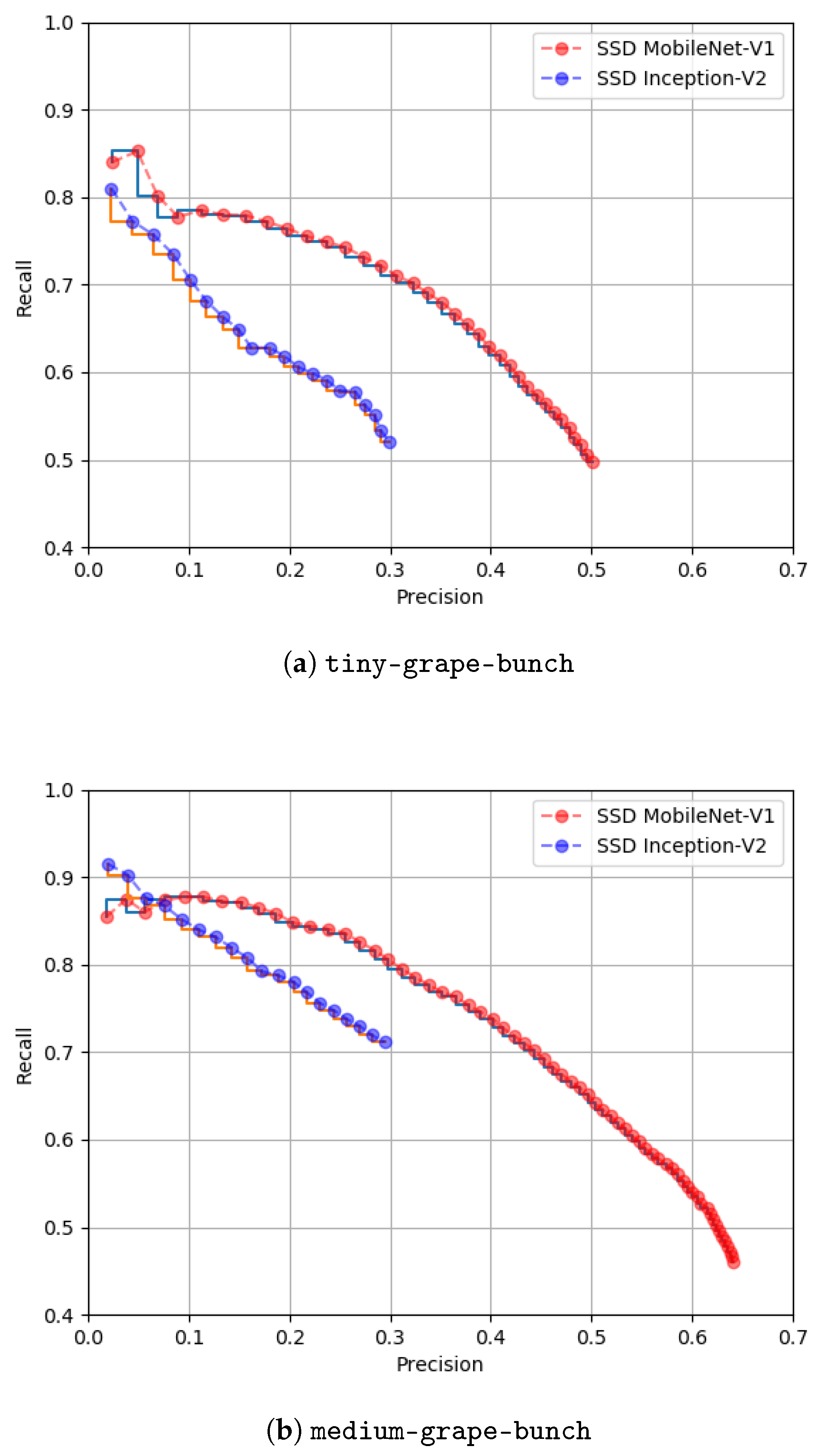
Figure 8 shows the precision × recall curves for both models considering the two classes and a confidence score of 50%.
Once again, this figure shows that SSD MobileNet-V1 outperformed the Inception model. Comparing the models performance detecting objects of both classes, we verified that detecting grape bunches at an early stage (tiny-grape-bunch) was more challenging than at an intermediate growth stage (medium-grape-bunch). The first class represented smaller grape bunches, with a color and texture more similar to the surrounding foliage, which complicated their detection. SSD MobileNet-V1 presented a AP of 40.38% detecting grape bunches at an early growth stage and 49.48% at an intermediate growth stage. Finally, Figure 9 shows the impact of the confidence score on the detections for a single image.
One can verify that this parameter can be used to eliminate FPs that usually present low-confidence scores.
Table 5 presents the detection performance considering a variation of the IoU evaluation parameter.
This characterization was performed since different values for the overlap between detections and ground truths can give more information about the models’ performance. For example, lower IoU values would consider detections that, besides not corresponding exactly to the location of the ground truths, represent annotated objects that were actually detected. To evaluate this, three values for the IoU parameter were considered: 20%, 40%, and 60%. Once again, one can verify that the SSD Inception-V2 model presented a higher precision. For an IoU value of 20%, this model had a precision of 92.57% detecting grape bunches at an intermediate growth stage. This is a satisfactory result since it means that 92.57% of the detections were TPs. On the other side, SSD MobileNet-V1 presented high recall levels. For an IoU of 20%, it achieved a recall of 87.01% for the class medium-grape-bunch. For higher IoU values, the performance of both models decreased. This was expected since, for example, for an IoU of 60%, the detections that did not overlap more than 60% with the ground truths were considered as FPs, which led to a decrease in performance. Overall, the best result was achieved by SSD MobileNet-V1, which performed with a mAP of 66.96% for an IoU of 20%.
As referenced before, the models were deployed in a low-cost and low-power embedded device, a TPU. It was intended that these models run in a time-effective manner to be integrated in more complex systems such as harvesting and spraying procedures. Thus, evaluating the runtime performance of both models was important in the context of this work. Table 6 shows the inference time results for both models.
In this table, the performances per tile and per image are both described. The inference time per tile was also considered in this evaluation since it represents the time that each model would take to process an entire image if the input images were not split. The inference times were measured for each evaluation image, and the final value considered was the average for all images. The results showed that the SSD MobileNet-V1 was more than four-times faster than the Inception model. This was due to the simpler architecture of MobileNets in relation to Inception, and the higher compatibility of MobileNet compared with Inception. This model can process a single tile in 6.29 ms and an entire split image in 93.12 ms. This proved both the high performance of the model, but also that the TPU hardware device used was capable of deploying models in a very efficient way, even considering low-power costs.
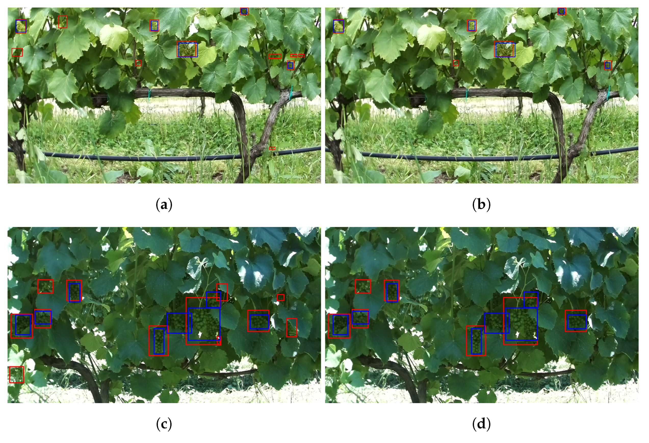
This approach was intended to be robust to different light conditions since the robot would operate at different times of the day and stages of the year. Because of this reason, the built dataset considered several light conditions, and the models were trained to be robust to them. Furthermore, the dataset considered occluded grape bunches so that the models could also detect not fully visible grape bunches. To demonstrate these challenging conditions present in the proposed dataset, Figure 10 and Figure 11 present an overview of the performance of SSD MobileNet-V1 considering occlusions in the grape bunches and variation in the illumination conditions.
For the models to be able to accommodate these conditions, the annotation procedure was crucial. In this process, the decision to consider occluded objects was made. Several times, the annotation of an occluded object was complex since there was the need to consider parts of other objects inside the bounding box corresponding to the occluded object. Figure 10 shows that occluded objects were taken into consideration during the annotation procedure and that the models were able to identify these objects in the images. Regarding the variations of the illumination conditions, one of the key steps to accomplish this goal was the capture of visual data during different days and stages of the year. To build the proposed dataset, the robot represented in Figure 1 was taken four times to the vineyard in order to capture the crop state in different conditions. The visit dates were 11 May 2021, 27 May 2021, 23 June 2021, and 26 July 2021.
On each day, images were recorded both in the morning and during the evening to account for multiple light conditions. In May, grape bunches at an early growth stage were captured, while in June and July, the intermediate growth stage was present in the vineyard. After recording all these data, the annotation process was once again essential since during the annotation, the objects were present under different light conditions. Figure 11 shows the different levels of illumination captured during the field visits performed. This figure proves that the models were able to detect grape bunches at different growth stages in these conditions.

4.3. Discussion

This work proposed a novel dataset for grape bunch detection at different growth stages. Two state-of-the-art models were used to perform this detection. Due to the requirement of a time-effective, low-power, and low-cost detection, this work used lightweight models that were quantized to be deployed in an embedded device. Quantization was used to reduce the size of the DL models and improve runtime performance by taking advantage of high throughput integer instructions. However, quantization can reduce the detection performance of DL models. Wu et al. [51] showed that the error rates increase when the model size decreases by quantization. In this work, this decrease in detection performance was accepted due to the high gain in runtime performance. In comparison with state-of-the-art works such as the one proposed by Palacios et al. [30], which detected grape flower at the bloom with an F1 score of 73.0%, this work presented a lower detection performance. On the other hand, the tradeoff between detection performance and runtime performance was extremely satisfactory since, especially for SSD MobileNet-V1, the model could perform with a mAP up to 66.96%, performing the detection at a rate higher than 10 Hz per image. In addition, the models were able to detect grape bunches at different stages, considering occlusions and variations in illumination conditions. Since the proposed dataset is publicly available, we believe that it has potential to be used in the future by the scientific community to train more complex and nonquantized DL models in order to achieve higher detection performances for applications without runtime restrictions. Furthermore, the proposed system can be adopted in future works and applications since it is cost-effective, portable, low-power, and independent of light conditions. The solution is modular and can be placed in any robotic platform, meaning that the price of the module is completely independent of the platform where it is placed. For applications that require higher levels of detection precision and that are not dependent on a time-effective solution, more complex models can be trained with the proposed dataset. Some works may also propose new DL-based architectures or modify state-of-the-art models to better suit the application purposes. For example, Taheri-Garavand et al. [11] proposed a modification to the VGG16 model to identify chickpea varieties by using seed images in the visible spectrum, and Nasiri et al. [12] proposed a similar approach to automate grapevine cultivar identification.
One of the main goals of this work was to achieve a low-power solution. The device used operates at high inference rate with a requirement of 5 V and 500 mA. This result was aligned with the state-of-the-art works that proposed advanced solutions for object detection using accelerator devices. Kaarmukilan et al. [52] used Movidius Neural Compute Stick 2, which similar to the TPU used in this work, is connected to the host device by USB and is capable of 4 TOPS with a 1.5 W power consumption. Dinelli et al. [53] compared several field-programmable gate array families by Xilinx and Intel for object detection. From all the evaluated devices, the authors achieved a minimum power consumption of 0.969 W and a maximum power consumption of 4.010 W.

5. Conclusions

This work approached the problem of detecting grape bunches at different growth stages by cameras mounted onboard mobile robots. A novel dataset with 1929 images and respective annotations was proposed considering different stages of grape bunches, constructed by visiting a vineyard four different times to record the data. To achieve time-effective, low-cost, and low-power grape bunch detection, two models were trained, quantized, and deployed in an embedded device. The results showed that the tradeoff between detection and runtime performance was satisfactory. SSD MobileNet-V1 achieved the best results, with a maximum detection performance of 66.96% and a runtime average cycle of 6.29 ms and 93.12 ms per tile and image, respectively.
In future work, we would like to extend the dataset to consider more grape bunch growth stages. Since our robotic platform was intended to run also at night, we will also consider including vineyard images captured at night using artificial illumination. Furthermore, we would like to test the proposed system in vineyards that were not considered in this work, to evaluate if the models are robust to different scenarios. Additionally, the proposed dataset could be extended to consider grape bunches of these different vineyards.

Author Contributions

Conceptualization, A.S.A., S.A.M. and F.N.d.S.; methodology, A.S.A., S.A.M., F.N.d.S., T.P., L.C. and J.V.; software, A.S.A., S.A.M. and L.C.; validation, F.N.d.S., T.P., J.V., R.M. and J.B.-C.; formal analysis, F.N.d.S., T.P., J.V., R.M. and J.B.-C.; investigation, A.S.A., S.A.M., F.N.d.S. and J.V.; resources, F.N.d.S.; data curation, A.S.A. and S.A.M.; writing—original draft preparation, A.S.A., S.A.M. and F.N.d.S.; writing—review and editing, F.N.d.S., L.C., T.P., J.V., R.M. and J.B.-C.; visualization, A.S.A., S.A.M., F.N.d.S., L.C., T.P., J.V., R.M. and J.B.-C.; supervision, F.N.d.S., J.V., R.M. and J.B.-C.; project administration, F.N.d.S.; funding acquisition, F.N.d.S. All authors have read and agreed to the published version of the manuscript.

Funding

This research was funded by “Metbots-Metabolomic Robots with Self-learning Artificial Intelligence for Precision Agriculture” Reference PTDC/EEI-ROB/31124/2017 and FEDER funds through the COMPETE 2020 Programme under Project Number POCI-01-0145-FEDER-031124.

Institutional Review Board Statement

Not applicable.

Informed Consent Statement

Not applicable.

Data Availability Statement

The data presented in this study are openly available in https://doi.org/10.5281/zenodo.5114142 (accessed on 1 August 2021).

Acknowledgments

André Silva Pinto de Aguiar thanks the FCT—Foundation for Science and Technology, Portugal, for the Ph.D. Grant DFA/BD/5318/2020. Sandro Augusto Magalhães thanks the FCT—Foundation for Science and Technology, Portugal, for the Ph.D Grant SFRH/BD/147117/2019. Martins RC acknowledges the Fundação para a Ciência e Tecnologia (FCT) research contract grant (CEEIND/017801/2018).

Conflicts of Interest

The authors declare no conflict of interest.

References

  1. Duckett, T.; Pearson, S.; Blackmore, S.; Grieve, B.; Chen, W.H.; Cielniak, G.; Cleaversmith, J.; Dai, J.; Davis, S.; Fox, C.; et al. Agricultural Robotics: The Future of Robotic Agriculture. arXiv 2018, arXiv:cs.RO/1806.06762. [Google Scholar]
  2. Billingsley, J.; Visala, A.; Dunn, M. Robotics in Agriculture and Forestry. In Springer Handbook of Robotics; Siciliano, B., Khatib, O., Eds.; Springer: Berlin/Heidelberg, Germany, 2008; pp. 1065–1077. [Google Scholar] [CrossRef] [Green Version]
  3. Andresen, T.; de Aguiar, F.B.; Curado, M.J. The Alto Douro Wine Region greenway. Landsc. Urban Plan. 2004, 68, 289–303. [Google Scholar] [CrossRef]
  4. Patrício, D.I.; Rieder, R. Computer vision and artificial intelligence in precision agriculture for grain crops: A systematic review. Comput. Electron. Agric. 2018, 153, 69–81. [Google Scholar] [CrossRef] [Green Version]
  5. Bargoti, S.; Underwood, J.P. Image segmentation for fruit detection and yield estimation in apple orchards. J. Field Robot. 2017, 34, 1039–1060. [Google Scholar] [CrossRef] [Green Version]
  6. LeCun, Y.; Bengio, Y.; Hinton, G. Deep learning. Nature 2015, 521, 436–444. [Google Scholar] [CrossRef]
  7. Schmidhuber, J. Deep learning in neural networks: An overview. Neural Netw. 2015, 61, 85–117. [Google Scholar] [CrossRef] [Green Version]
  8. Santos, L.; Santos, F.N.; Oliveira, P.M.; Shinde, P. Deep Learning Applications in Agriculture: A Short Review. In Proceedings of the Robot 2019: Fourth Iberian Robotics Conference, Porto, Portugal, 20–22 November 2020; Silva, M.F., Luís Lima, J., Reis, L.P., Sanfeliu, A., Tardioli, D., Eds.; Springer: Cham, Switzerland, 2020; pp. 139–151. [Google Scholar]
  9. Kamilaris, A.; Prenafeta-Boldú, F.X. Deep learning in agriculture: A survey. Comput. Electron. Agric. 2018, 147, 70–90. [Google Scholar] [CrossRef] [Green Version]
  10. Kamilaris, A.; Prenafeta-Boldú, F.X. A review of the use of convolutional neural networks in agriculture. J. Agric. Sci. 2018, 156, 312–322. [Google Scholar] [CrossRef] [Green Version]
  11. Taheri-Garavand, A.; Nasiri, A.; Fanourakis, D.; Fatahi, S.; Omid, M.; Nikoloudakis, N. Automated In Situ Seed Variety Identification via Deep Learning: A Case Study in Chickpea. Plants 2021, 10, 1406. [Google Scholar] [CrossRef]
  12. Nasiri, A.; Taheri-Garavand, A.; Fanourakis, D.; Zhang, Y.D.; Nikoloudakis, N. Automated Grapevine Cultivar Identification via Leaf Imaging and Deep Convolutional Neural Networks: A Proof-of-Concept Study Employing Primary Iranian Varieties. Plants 2021, 10, 1628. [Google Scholar] [CrossRef] [PubMed]
  13. Wang, X.; Han, Y.; Wang, C.; Zhao, Q.; Chen, X.; Chen, M. In-Edge AI: Intelligentizing Mobile Edge Computing, Caching and Communication by Federated Learning. IEEE Netw. 2019, 33, 156–165. [Google Scholar] [CrossRef] [Green Version]
  14. Pinto de Aguiar, A.S.; Neves dos Santos, F.B.; Feliz dos Santos, L.C.; de Jesus Filipe, V.M.; Miranda de Sousa, A.J. Vineyard trunk detection using deep learning—An experimental device benchmark. Comput. Electron. Agric. 2020, 175, 105535. [Google Scholar] [CrossRef]
  15. Aguiar, A.S.; Santos, F.N.D.; De Sousa, A.J.M.; Oliveira, P.M.; Santos, L.C. Visual Trunk Detection Using Transfer Learning and a Deep Learning-Based Coprocessor. IEEE Access 2020, 8, 77308–77320. [Google Scholar] [CrossRef]
  16. Aguiar, A.S.; Monteiro, N.N.; Santos, F.N.d.; Solteiro Pires, E.J.; Silva, D.; Sousa, A.J.; Boaventura-Cunha, J. Bringing Semantics to the Vineyard: An Approach on Deep Learning-Based Vine Trunk Detection. Agriculture 2021, 11, 131. [Google Scholar] [CrossRef]
  17. Magalhães, S.A.; Castro, L.; Moreira, G.; dos Santos, F.N.; Cunha, M.; Dias, J.; Moreira, A.P. Evaluating the Single-Shot MultiBox Detector and YOLO Deep Learning Models for the Detection of Tomatoes in a Greenhouse. Sensors 2021, 21, 3569. [Google Scholar] [CrossRef] [PubMed]
  18. Fanourakis, D.; Kazakos, F.; Nektarios, P.A. Allometric Individual Leaf Area Estimation in Chrysanthemum. Agronomy 2021, 11, 795. [Google Scholar] [CrossRef]
  19. Taheri-Garavand, A.; Nejad, A.R.; Fanourakis, D.; Fatahi, S.; Majd, M.A. Employment of artificial neural networks for non-invasive estimation of leaf water status using color features: A case study in Spathiphyllum wallisii. Acta Physiol. Plant. 2021, 43, 78. [Google Scholar] [CrossRef]
  20. Dias, P.A.; Tabb, A.; Medeiros, H. Apple flower detection using deep convolutional networks. Comput. Ind. 2018, 99, 17–28. [Google Scholar] [CrossRef] [Green Version]
  21. Koirala, A.; Walsh, K.B.; Wang, Z.X.; McCarthy, C. Deep learning for real-time fruit detection and orchard fruit load estimation: Benchmarking of ‘MangoYOLO’. Precis. Agric. 2019, 20, 1–29. [Google Scholar] [CrossRef]
  22. Redmon, J.; Divvala, S.; Girshick, R.; Farhadi, A. You Only Look Once: Unified, Real-Time Object Detection. In Proceedings of the IEEE Conference on Computer Vision and Pattern Recognition (CVPR), Las Vegas, NV, USA, 26 June–1 July 2016. [Google Scholar]
  23. Zheng, Y.Y.; Kong, J.L.; Jin, X.B.; Wang, X.Y.; Su, T.L.; Zuo, M. CropDeep: The Crop Vision Dataset for Deep-Learning-Based Classification and Detection in Precision Agriculture. Sensors 2019, 19, 1058. [Google Scholar] [CrossRef] [Green Version]
  24. Bargoti, S.; Underwood, J. Deep fruit detection in orchards. In Proceedings of the 2017 IEEE International Conference on Robotics and Automation (ICRA), Singapore, 29 May–3 June 2017; pp. 3626–3633. [Google Scholar] [CrossRef] [Green Version]
  25. Ren, S.; He, K.; Girshick, R.; Sun, J. Faster R-CNN: Towards Real-Time Object Detection with Region Proposal Networks. arXiv 2015, arXiv:cs.CV/1506.01497. [Google Scholar] [CrossRef] [Green Version]
  26. Sa, I.; Ge, Z.; Dayoub, F.; Upcroft, B.; Perez, T.; McCool, C. DeepFruits: A Fruit Detection System Using Deep Neural Networks. Sensors 2016, 16, 1222. [Google Scholar] [CrossRef] [Green Version]
  27. Kirk, R.; Cielniak, G.; Mangan, M. L*a*b*Fruits: A Rapid and Robust Outdoor Fruit Detection System Combining Bio-Inspired Features with One-Stage Deep Learning Networks. Sensors 2020, 20, 275. [Google Scholar] [CrossRef] [Green Version]
  28. Liu, S.; Li, X.; Wu, H.; Xin, B.; Tang, J.; Petrie, P.R.; Whitty, M. A robust automated flower estimation system for grape vines. Biosyst. Eng. 2018, 172, 110–123. [Google Scholar] [CrossRef]
  29. Diago, M.P.; Sanz-Garcia, A.; Millan, B.; Blasco, J.; Tardaguila, J. Assessment of flower number per inflorescence in grapevine by image analysis under field conditions. J. Sci. Food Agric. 2014, 94, 1981–1987. [Google Scholar] [CrossRef] [PubMed]
  30. Palacios, F.; Bueno, G.; Salido, J.; Diago, M.P.; Hernández, I.; Tardaguila, J. Automated grapevine flower detection and quantification method based on computer vision and deep learning from on-the-go imaging using a mobile sensing platform under field conditions. Comput. Electron. Agric. 2020, 178, 105796. [Google Scholar] [CrossRef]
  31. Pérez-Zavala, R.; Torres-Torriti, M.; Cheein, F.A.; Troni, G. A pattern recognition strategy for visual grape bunch detection in vineyards. Comput. Electron. Agric. 2018, 151, 136–149. [Google Scholar] [CrossRef]
  32. Reis, M.; Morais, R.; Peres, E.; Pereira, C.; Contente, O.; Soares, S.; Valente, A.; Baptista, J.; Ferreira, P.; Bulas Cruz, J. Automatic detection of bunches of grapes in natural environment from color images. J. Appl. Log. 2012, 10, 285–290. [Google Scholar] [CrossRef] [Green Version]
  33. Liu, S.; Whitty, M. Automatic grape bunch detection in vineyards with an SVM classifier. J. Appl. Log. 2015, 13, 643–653. [Google Scholar] [CrossRef]
  34. Cecotti, H.; Rivera, A.; Farhadloo, M.; Pedroza, M.A. Grape detection with convolutional neural networks. Expert Syst. Appl. 2020, 159, 113588. [Google Scholar] [CrossRef]
  35. Santos, T.T.; de Souza, L.L.; dos Santos, A.A.; Avila, S. Grape detection, segmentation, and tracking using deep neural networks and three-dimensional association. Comput. Electron. Agric. 2020, 170, 105247. [Google Scholar] [CrossRef] [Green Version]
  36. Xiong, J.; Liu, Z.; Lin, R.; Bu, R.; He, Z.; Yang, Z.; Liang, C. Green Grape Detection and Picking-Point Calculation in a Night-Time Natural Environment Using a Charge-Coupled Device (CCD) Vision Sensor with Artificial Illumination. Sensors 2018, 18, 969. [Google Scholar] [CrossRef] [PubMed] [Green Version]
  37. Kangune, K.; Kulkarni, V.; Kosamkar, P. Grapes Ripeness Estimation using Convolutional Neural network and Support Vector Machine. In Proceedings of the 2019 Global Conference for Advancement in Technology (GCAT), Bangalore, India, 18–20 October 2019; pp. 1–5. [Google Scholar] [CrossRef]
  38. Aquino, A.; Millan, B.; Gutiérrez, S.; Tardáguila, J. Grapevine flower estimation by applying artificial vision techniques on images with uncontrolled scene and multi-model analysis. Comput. Electron. Agric. 2015, 119, 92–104. [Google Scholar] [CrossRef]
  39. He, K.; Zhang, X.; Ren, S.; Sun, J. Deep residual learning for image recognition. In Proceedings of the IEEE Conference on Computer Vision and Pattern Recognition (CVPR), Las Vegas, NV, USA, 26 June–1 July 2016; pp. 770–778. [Google Scholar]
  40. Everingham, M.; Van Gool, L.; Williams, C.K.; Winn, J.; Zisserman, A. The pascal visual object classes (voc) challenge. Int. J. Comput. Vis. 2010, 88, 303–338. [Google Scholar] [CrossRef] [Green Version]
  41. Computer Vision Annotation Tool (CVAT). Available online: https://github.com/openvinotoolkit/cvat (accessed on 6 August 2021).
  42. Tzutalin. LabelImg. Git Code. 2015. Available online: https://github.com/tzutalin/labelImg (accessed on 6 August 2021).
  43. Shorten, C.; Khoshgoftaar, T.M. A survey on Image Data Augmentation for Deep Learning. J. Big Data 2019, 6, 1–48. [Google Scholar] [CrossRef]
  44. Howard, A.G.; Zhu, M.; Chen, B.; Kalenichenko, D.; Wang, W.; Weyand, T.; Andreetto, M.; Adam, H. Mobilenets: Efficient convolutional neural networks for mobile vision applications. arXiv 2017, arXiv:1704.04861. [Google Scholar]
  45. Szegedy, C.; Vanhoucke, V.; Ioffe, S.; Shlens, J.; Wojna, Z. Rethinking the Inception Architecture for Computer Vision. arXiv 2015, arXiv:cs.CV/1512.00567. [Google Scholar]
  46. Liu, W.; Anguelov, D.; Erhan, D.; Szegedy, C.; Reed, S.; Fu, C.Y.; Berg, A.C. Ssd: Single shot multibox detector. In Proceedings of the European Conference on Computer Vision, Amsterdam, The Netherlands, 11–14 October 2016; Springer: Berlin/Heidelberg, Germany, 2016; pp. 21–37. [Google Scholar]
  47. Lin, T.Y.; Maire, M.; Belongie, S.J.; Hays, J.; Perona, P.; Ramanan, D.; Dollár, P.; Zitnick, C.L. Microsoft COCO: Common Objects in Context. In Proceedings of the ECCV 2014, Zurich, Switzerland, 6–12 September 2014. [Google Scholar]
  48. Abadi, M.; Barham, P.; Chen, J.; Chen, Z.; Davis, A.; Dean, J.; Devin, M.; Ghemawat, S.; Irving, G.; Isard, M.; et al. Tensorflow: A system for large-scale machine learning. In Proceedings of the 12th {USENIX} symposium on operating systems design and implementation ({OSDI} 16), Savannah, GA, USA, 2–4 November 2016; pp. 265–283. [Google Scholar]
  49. Tucker, G.; Wu, M.; Sun, M.; Panchapagesan, S.; Fu, G.; Vitaladevuni, S. Model Compression Applied to Small-Footprint Keyword Spotting. In Proceedings of the Interspeech 2016, San Francisco, CA, USA, 8–12 September 2016; pp. 1878–1882. [Google Scholar]
  50. Neubeck, A.; Van Gool, L. Efficient non-maximum suppression. In Proceedings of the 18th International Conference on Pattern Recognition (ICPR’06), Hong Kong, China, 20–24 August 2006; Volume 3, pp. 850–855. [Google Scholar]
  51. Wu, H.; Judd, P.; Zhang, X.; Isaev, M.; Micikevicius, P. Integer quantization for deep learning inference: Principles and empirical evaluation. arXiv 2020, arXiv:2004.09602. [Google Scholar]
  52. Kaarmukilan, S.; Hazarika, A.; Poddar, S.; Rahaman, H. An Accelerated Prototype with Movidius Neural Compute Stick for Real-Time Object Detection. In Proceedings of the 2020 International Symposium on Devices, Circuits and Systems (ISDCS), Howrah, India, 4–6 March 2020; pp. 1–5. [Google Scholar]
  53. Dinelli, G.; Meoni, G.; Rapuano, E.; Benelli, G.; Fanucci, L. An FPGA-Based Hardware Accelerator for CNNs Using On-Chip Memories Only: Design and Benchmarking with Intel Movidius Neural Compute Stick. Int. J. Reconfig. Comput. 2019, 2019, 1–13. [Google Scholar] [CrossRef] [Green Version]
Figure 1. Agricultural robot used to collect visual data with onboard cameras pointing to the canopy.
Agronomy 11 01890 g001
Figure 2. High-level workflow of the proposed system. The first step is data collection, where images are extracted and stored from videos recorded by onboard cameras. Then, the dataset is generated by the grape bunch annotation; data augmentation is performed to increase the dataset size; the images are split to improve the training performance. Finally, the models are trained, then quantized and compiled so that they can be deployed in a lightweight embedded device.
Agronomy 11 01890 g002
Figure 3. Two images of the proposed publicly available dataset considering (a) an early and (b) a medium grape bunch growth stage.
Agronomy 11 01890 g003
Figure 4. Set of augmentation operations applied to a single image to extend the original dataset.
Agronomy 11 01890 g004
Figure 5. Split of a collected image to a 300 × 300 px resolution. The original image with a resolution of 1920 × 1080 px generated 40 split images considering an overlapping ratio of 20%.
Agronomy 11 01890 g005
Figure 6. Steps to train and deploy a pretrained model into Google’s Coral USB Accelerator (TPU).
Agronomy 11 01890 g006
Figure 7. Impact of nonmaximum suppression on the final inference result.
Agronomy 11 01890 g007
Figure 8. Precision × recall curves for both models and both classes considering a confidence score of 50% and an IoU of 50%
Agronomy 11 01890 g008
Figure 9. Impact of the confidence score on the final detection results. Blue bounding boxes represent the ground truth and the red ones the SSD MobileNet-V1 detections considering a confidence score of (a,c) 20% and (b,d) 50%.
Agronomy 11 01890 g009
Figure 10. Detection of grape bunches (a) in early, and (b) intermediate growth stages considering occlusions caused by the dense foliage present in the vineyard. Blue bounding boxes represent the ground truth and the red ones the detections.
Agronomy 11 01890 g010
Figure 11. Demonstration of the differences in illumination captured by the proposed dataset and the corresponding ability of the models to deal with it. Each image (ad) represents a different light condition. Blue bounding boxes represent the ground truth and the red ones the detections.
Agronomy 11 01890 g011
Table 1. Summary of the current state-of-the-art of Deep-Learning (DL)-based grape detection.
ReferenceApplicationPerformance
Liu et al. [28] (2018)Automated grape flower counting to determine potential yields at early stages.Accuracy of 84.3% for flower estimation.
Diago et al. [29] (2014)Assessment of flower number per inflorescence in grapevine.Precision exceeding 90.0%.
Palacios et al. [30] (2020)Estimation of the number of flowers at the bloom.F1 score of 73.0% for individual flower detection.
Pérez-Zavala et al. [31] (2018)Grape bunch detection for automating grapevine growth monitoring, spraying, leaf thinning, and harvesting tasks.AP of 88.6% and Average Recall (AR) of 80.3%.
Reis et al. [32] (2012)Support harvesting procedures by grape bunch detection.97.0% and 91.0% correct classifications for red and white grapes.
Liu and Whitty et al. [33] (2015)Precise yield estimation in vineyards by detecting bunches of red grapes in images.Accuracy of 88.0% and recall of 91.6%.
Cecotti et al. [34] (2020)Study of the best CNN architecture to detect grapes in images.Accuracy of 99.0% for both red and white grapes.
Santos et al. [35] (2020)Infer the crop state for yield prediction, precision agriculture, and automated harvesting.F1 score of 91.0% for instance grape segmentation.
Xiong et al. [36] (2018)Develop a technology for night-time fruit picking using artificial illumination.Accuracy of 91.7% for green grape detection.
Kangune et al. [37] (2019)Grape ripeness estimation.Classification accuracy of 79.5% between ripened and unripened grapes.
Aquino et al. [38] (2015)Early yield prediction and flower estimation in vineyards.Precision and recall were 83.4% and 85.0%.
Table 2. Description of the augmentation operations used to expand the original collection of data.
Augmentation OperationDescription
RotationRotates the image by +30 and −30 degrees.
TranslationTranslates the image by −30% to +30% on the x- and y-axis.
ScaleScales the image to a value of 50 to 150% of their original size.
FlippingMirrors the image horizontally.
MultiplyMultiplies all pixels in an image with a random value sampled once per image,
which can be used to make images lighter or darker.
Table 3. Number of annotated objects per class. The original dataset contains 1929 images with two different classes. To increase the dataset size, several augmentation operations were applied, increasing the number of images to 13,503. Finally, the images were split, and the final dataset was composed of 302,252 images.
Class# of Objects# of Objects in Augmented Images# of Objects in Split Images
tiny_grape_bunch249713,39325,349
medium_grape_bunch429225,18951,272
Table 4. Grape bunch detection performance considering an IoU of 50% and a variation of the confidence threshold for three different values.
ModelConfidence (%)ClassPrecision (%)Recall (%)F1 Score (%)AP (%)mAP (%)
SSD MobileNet-V130tiny-grape-bunch17.3861.7227.1240.3844.93
medium-grape-bunch28.5366.4439.9249.48
SSD Inception-V230tiny-grape-bunch35.8144.8839.8326.9528.32
medium-grape-bunch64.6237.5947.5329.68
SSD MobileNet-V150tiny-grape-bunch49.2850.4449.8536.2942.47
medium-grape-bunch45.5964.2653.3448.64
SSD Inception-V250tiny-grape-bunch51.3630.5738.3320.5022.48
medium-grape-bunch70.8629.9042.0624.45
SSD MobileNet-V170tiny-grape-bunch78.1211.8520.589.8622.45
medium-grape-bunch71.9541.9953.0335.04
SSD Inception-V270tiny-grape-bunch67.1712.0520.449.3012.19
medium-grape-bunch79.1217.4628.6015.08
Table 5. Grape bunch detection performance considering a confidence of 50% and a variation of the IoU threshold for three different values.
ModelIoU (%)ClassPrecision (%)Recall (%)F1 Score (%)AP (%)mAP (%)
SSD MobileNet-V120tiny-grape-bunch63.7365.2264.4756.8766.96
medium-grape-bunch61.7287.0172.2277.05
SSD Inception-V220tiny-grape-bunch71.9042.8053.6636.4237.22
medium-grape-bunch92.5739.0654.9438.01
SSD MobileNet-V140tiny-grape-bunch57.1758.5157.8347.0155.78
medium-grape-bunch54.9677.4764.3064.55
SSD Inception-V240tiny-grape-bunch64.2538.2447.9530.5031.98
medium-grape-bunch85.1435.9350.5333.45
SSD MobileNet-V160tiny-grape-bunch37.5438.4137.9722.3924.79
medium-grape-bunch32.1745.3437.6427.19
SSD Inception-V260tiny-grape-bunch33.3819.8724.918.729.79
medium-grape-bunch45.7819.3227.1710.85
Table 6. Runtime performance of both models.
ModelInference Time per Tile (ms)Inference Time per Image (ms)
SSD MobileNet-V16.2993.12
SSD Inception-V226.07385.69
Publisher’s Note: MDPI stays neutral with regard to jurisdictional claims in published maps and institutional affiliations.

