1. Introduction
With yield being considered a quality grape and wine indicator [
1,
2,
3,
4,
5], it is crucial to obtain an early estimation of the quantity of grapes per area unit. Knowing in advance vineyard yield is a key issue so that growers and winemakers can achieve the best balance between vegetative and reproductive growth, make more informed decisions as to thinning, irrigation, and nutrient management, schedule harvest, optimize winemaking operations, program crop insurance, and grape picking workforce demand, and help fraud detection [
6,
7,
8].
The traditional methods [
9] are considered destructive, labor-demanding, and time-consuming [
4], with low accuracy [
10] primarily due to operator errors [
11] and sparse sampling (when compared to the inherent spatial variability in a production vineyard [
5,
12]). These are supported by manual sampling, where yield is estimated by sampling clusters weight and the number of clusters per vine, historical data, and extrapolation considering the number of vines in a plot. The main efforts towards improved yield models applied to the vineyard, considered one of the most complex phenotypic traits in viticulture [
13], are in most cases focused on image analysis for grape detection at field level, with a significant drawback derived from cluster occlusion [
14,
15].
The growing adoption of Precision Agriculture (PA) practices, closely related with the ongoing advances in Geospatial Technologies (GT), Remote Sensing (RS), Proximal Sensing (PS), Internet of Things (IoT), Unmanned Aerial Vehicles (UAVs), Big Data Analytics (BDA) and Artificial Intelligence (AI) [
16,
17,
18,
19], are fueling the particular application in Precision Viticulture (PV) [
20] where the importance of the wine industry drives the development of innovative methods and technologies to cope with the heterogeneity within vineyards that results from high inter-annual and spatial variability derived from the effects of soil and climate conditions, grapevine variety, biotic and abiotic stresses, vineyard management practices, among others [
18,
21]. However, despite being a hot topic in research over recent years, it still lacks solutions that can transfer the acquired knowledge and methods to the field and provide tools for wine-growers decision support.
Models based on statistically significant relationships between predictors and grapevine parameters are increasingly being overtaken by crop models that can dynamically simulate and integrate into different time frames, plant traits, and other variables regarding management, soil, and climate data [
22]. This is particularly relevant, as grape production for wine is closely related to climate variables characterized in the past years by high inter-annual variability with direct adverse effects for wine producers that tend to be amplified by future climate changes’ perceived scenarios [
23,
24,
25,
26]. Nowadays, zoning the wine production areas, especially in denomination areas, is increasingly becoming more critical for the identification and characterization of homogenous areas that are the basis of regulatory measures over wine [
8], to allow marketing strategies regarding controlled origins [
27], and also regarding climate changes that require decisions at a regional level concerning adaptability of different varieties and mitigation management options in one of the most important crops in Europe [
28]. PV must apply at the field level and at a larger scale, where the spatial variability may reveal general trends of variation not perceived at more minor scales [
29].
The purpose of this present paper is three-fold: first, to perceive the research approaches for predicting yield in vineyards for wine production that can serve as an alternative to traditional estimation methods; second, to characterize the different new approaches identifying and comparing their applicability under field conditions, scalability concerning the objective, accuracy, advantages and shortcomings, and third, to identify research gaps for future developments and support a future research agenda on this topic. To achieve this goal, a systematic literature review was conducted using the PRISMA statement as a guideline [
30].
2. Methodology
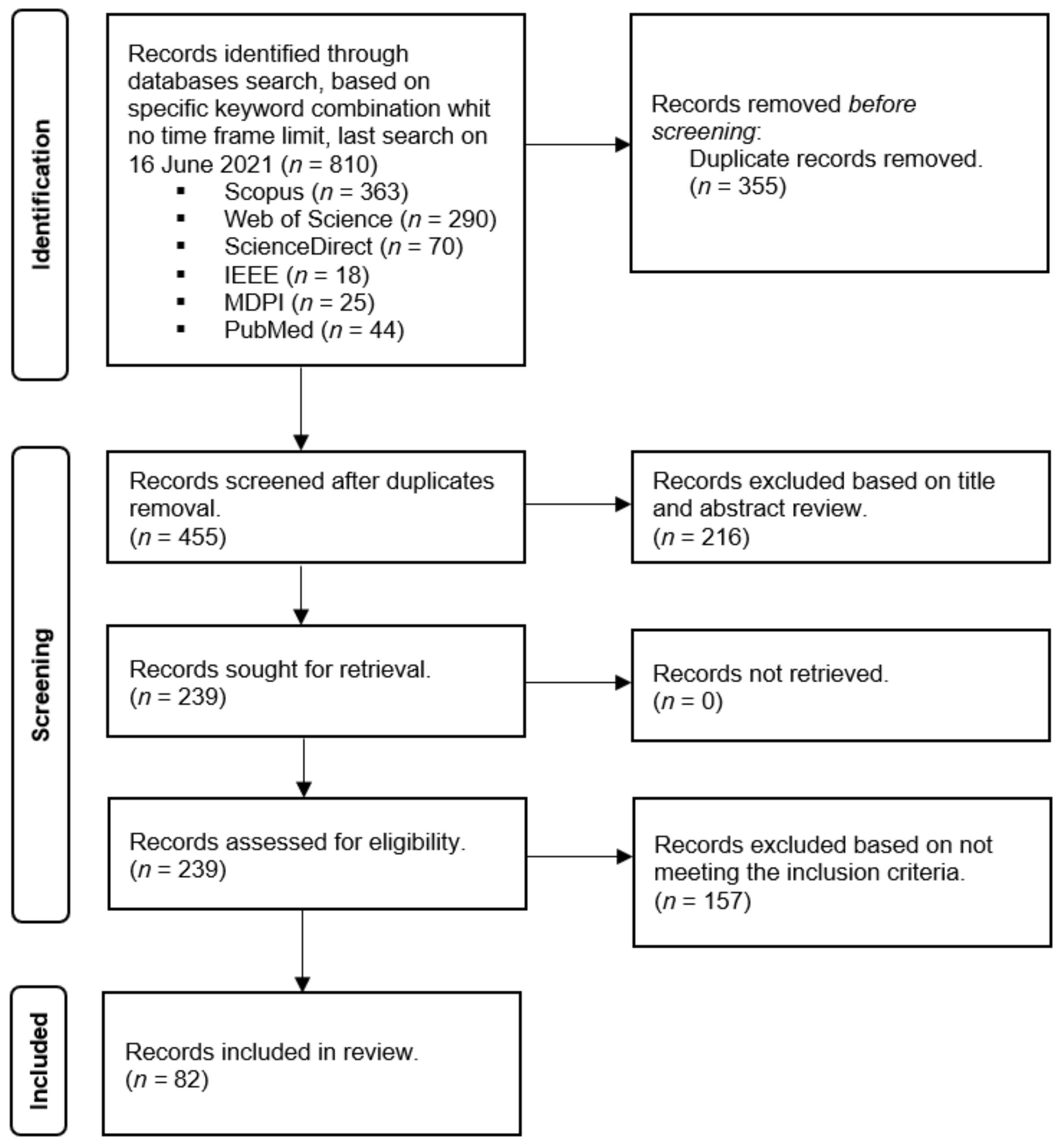
To identify the relevant scientific work already published on vineyard yield estimation, prediction, and forecasting, the authors carried out a systematic literature review of academic articles indexed on the Scopus, Web of Science, ScienceDirect, IEEE, MDPI, and PubMed databases, using the Preferred Reporting Items for Systematic Reviews and Meta-analyses (PRISMA) statement as a guideline [
30]. Other databases such as Google Scholar and ResearchGate were not considered because a preliminary study undertaken by the authors showed that they would only contribute to a significant increase in duplicate articles.
Depending on the approach, the terminology behind knowing as far in advance as possible the quantity of grapes that will be harvested can be referred to as (1) estimation—when the goal is to find the most suitable parameter that best describes a multivariate distribution of a historical dataset, (2) as prediction—when a dataset is used to compute random values of the unseen data, and (3) as forecasting—when a temporal dimension in a prediction problem is explicitly added. In the present review, the authors adopted the broader term of yield estimation, although the other terms were considered keywords in the search criteria.
The authors adopted a search criteria query string conducted on the title, abstract, and keywords, using all the combinations of the following keywords: “yield” OR “production” AND “estimation” OR “prediction” OR “forecasting” AND “vineyard” OR “grapevine”. Only peer-reviewed journals, conference articles, and book chapters were considered for screening.
As the goal is to perceive alternatives to the traditional manual sampling method of determining in advance the vineyard yield, those were excluded from the final data set.
A total of 455 articles published between 1981 and 2021 were found. These articles were reviewed firstly based on title and abstract meeting the search criteria with the inclusion of the indicated keywords, resulting in 239 articles that were retrieved from the respective databases. Further reading resulted in the final 82 records included in the review that verify the research criteria for including scientific studies for vineyard yield estimation, prediction, and forecasting. (
Figure 1).
The final record data set was categorized based on ten different methodological approaches identified for yield estimation in the screening phase that fall into a broader group of indirect estimation models derived mainly from dynamic or crop simulation models and data-driven models. Those were subdivided according to what can be considered more specific approaches: A—data-driven models based on computer vision and image processing; B—data-driven models based on vegetation indices; C—data-driven models based on pollen; D—crop simulation models; E—data-driven models based on trellis tension; F—data-driven models based on laser data processing; G—data-driven models based on radar data processing; H—data-driven models based on RF data processing; I—data-driven models based on ultrasonic signal processing; J—other data-driven models. Data regarding the year, journal distribution, data sources, test environment, applicability scale, and related variables used in estimation and accuracy were evaluated for each methodological approach. The abbreviations and acronyms used are listed on
Table 1.
3. Results and Discussion
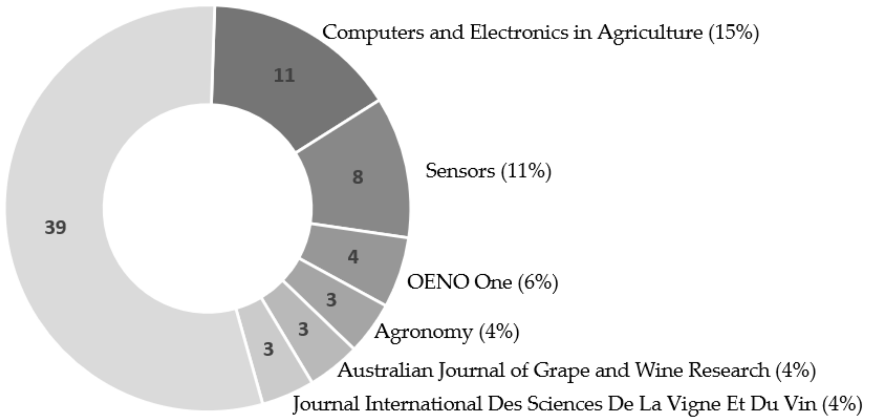
Looking at the scientific peer-reviewed journal distributions (
Figure 2) it is interesting to see the vast scope of this topic in the researcher’s community with publications in 38 different journals, most of them with diverse subjects and scopes, ranging from agronomy to robotics, climate, and sensors. The top six cover 45% of the total papers published, with the remaining 39 (55%) published in 32 different journals.
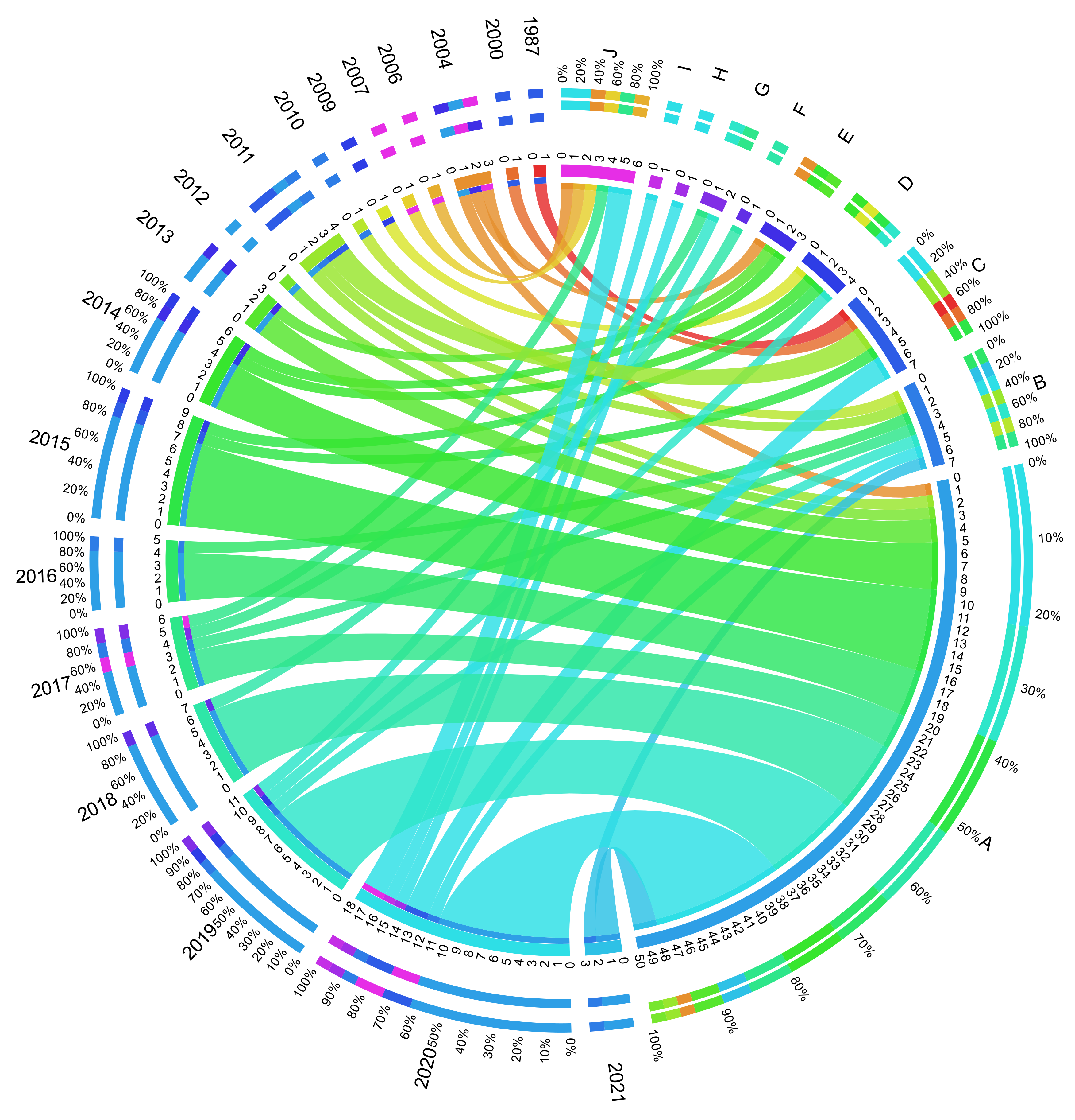
For an overall perception of the ten different methodological approaches identified for yield estimation, they are represented in
Figure 3, created with Circos [
31].
On the right side of the semicircle, we can see the methodologies (from A to J), and on the left side, the years of the publications (from 1987 to 2021-not considering years in which there are no identified records). The included records are arranged circularly in segments and joined with scaled and colored thickness ribbons to relate the year of publication with the different methodological approaches quantitatively. The relationship between both appears in the inner circle. The thickness and the color represent the percentage of the relationship. Taking the year 2020 as an example, we can see that a universe of 18 records was included in the present review. From those, 11 (61% of the year 2020 records) are related to A (data-driven models based on image processing algorithms), representing 22% of the 50 records on data-driven models based on image processing algorithms. Visually we can see that since 2009, there has been a continuous production of articles on this topic, with an increasing interest in research since 2018 with a peak in 2020 (for 2021, the data only covers five months). Regarding methodological approaches, the focus of the researchers dealing with this complex topic is on data-driven models based on image processing algorithms (A) (61%), followed by data-driven models based on vegetation indices (B) (9%) and data-driven models based on pollen (C) (9%).
Crop yield estimation has a high degree of complexity. It involves, in most cases, the characterization of driving factors related to climate, plant, and crop management [
32] that directly influence the number of clusters per vine, berries per cluster, and berry weight, as the three yield components [
12], explaining 60%, 30% and 10% of the yield respectively [
24,
33].The different general methodological approaches used for vineyard yield estimation can be divided firstly regarding the scale (in-field level vs. regional level), and secondly, by direct (based on manual sampling) or indirect methods (statistical models, regression models, proximal/remote sensing, and dynamic or crop simulation models) that depend primarily on image identification and/or related climate, soil, vegetation, and crop management variables [
32,
34,
35] that can also support crop simulation models, data-driven [
23] and mechanistic growth models [
36].
The standard or traditional methods retrieve limited data and produce a static prediction in a multi-step process of determining average number of clusters per vine, number of berries per cluster, and weight per cluster or berry with the growth overall 10% error greatly dependent on adequate staffing and extensive historical databases of cluster weights and yields [
37]
Computer vision and image processing are leading the alternative methods and are one of the most utilized techniques for attempting an early yield estimation. Still, different approaches such as Synthetic Aperture Radar (SAR), low frequency ultrasound [
38], RF Signals [
39], counting number of flowers [
40,
41,
42,
43,
44,
45,
46,
47], Boolean model application [
48], shoot count [
49], shoot biomass [
50,
51], frequency-modulated continuous-wave (FMCW) radar [
52,
53], detection of specular spherical reflection peaks [
54], the combination of RGB and multispectral imagery [
55] along with derived occlusion ratios, are alternative methods.
Whatever the indirect method used, they all allow a fast and non-invasive alternative to manual sampling. They allow identifying single berries in images, even taken from a simple device such as a smartphone [
56,
57,
58] and then using different methods such as convolutional neural networks [
1,
59], cellular automata [
60], or even sensors capable of collecting phenotypic traits of grape bunches, that are known to be related with grapevine yield [
14,
61], to estimate yields.
Approaches such as non-productive canopy detection using green pixel thresholding in video frames, local thresholding and Self-Organizing-Maps on aerial imagery [
62], light detection and ranging (LiDAR) for vineyard reconstruction [
63], and map pruning wood [
64] do not allow direct estimation of the yield but instead provide data layers to relate or use directly or as a correction coefficient in other methodologies, as they can show a relationship to yield.
Indices have been experiencing exponential growth in research related to productive and vegetative parameters in vineyards [
65,
66]. Derived from satellite imagery, UAVs [
65,
67], Unmanned Ground Vehicles (UGVs), or those mounted on tractors and Utility Terrain Vehicles (UTVs)[
68], Normalized Difference Vegetation Index (NDVI)[
11], Leaf Area Index (LAI) [
5,
68] and Water Index (WI) (with added importance in rainfed vineyards where water deficits play a significant role) [
69], are predictors of spatial yield variability using passive and/or active sensors.
Other indirect methods include Bayesian growth models [
70], weather-based models [
71], models based on a combination of variables (meteorological, phenological and phytopathological) [
6,
72], dynamic crop models such as the “Simulateur mulTIdisciplinaire pour les Cultures Standard” (STICS) [
73,
74], crop biometric maps [
75], and the continuous measurement of the tension in the horizontal (cordon) support wire of the trellis [
37,
76,
77], also used to determine the best moment of hand sampling for yield estimation [
78].
Predicting yield at a larger scale makes more sense now than ever as inter-annual variations attributed to climate change are entering a complex equation where quality, sustainability, efficiency, commercial and marketing strategies, regulations, insurances, stock management, and quotas are all related to yield forecasting [
24]. However, at a regional level, there are few examples of yield forecasting. Those can be divided mainly into climate-based models estimating grape and wine production [
23,
79,
80,
81], pollen-based models [
24,
82,
83,
84], a combination of one or both with phenological and phytopathological variables [
6,
8], STICS models [
74], and models based on correlations with indices such as NDVI, LAI, and NDWI [
85].
Harvest estimation is a problem to which machine learning, computer vision, and image processing can be applied using one or a combination of techniques [
86,
87,
88]. In proximal sensing methods, detection, segmentation, and counting of either individual grapes or bunches are complex in most image-based methodologies [
38,
59,
89], especially in non-disturbed canopies where occlusion [
15,
90], illumination, colors, and contrast [
91,
92] are challenging and in most cases are only demonstrated conceptually at a small scale [
89].
Along with Data Science, Artificial Intelligence, and Deep Learning, vineyard yield estimation can be applied at larger scales, not only through image analysis algorithms but also by identifying relevant predictive variables using data associated with climate, yield, phenology, fertilization, soil, maturation [
23,
40] and diseases [
93], by making use of a growing number of remote sensing [
85] and phenotyping platforms that allow quantitatively assessing plant traits in which yield falls [
94,
95].
3.1. A-Data-Driven Models Based on Computer Vision and Image Processing (n = 50)
Table 2 shows the summary of the records included in the systematic review regarding the use of computer vision and image processing techniques for yield estimation based on image, recorded mainly with still or mounted standard Red, Green, and Blue (RGB) and RGB-Depth Sensor (D) cameras, for the most under field conditions with a local application scale. The main goal is to extract variables from the images that can be related to the actual yield, such as the number of berries, bunch/cluster area, leaf area, number of flowers, stems, and branches. This can be accomplished with various computer vision, machine learning, and deep learning approaches.
From the retrieved results, we can say that computer vision and image processing are the most utilized techniques for attempting an early yield estimation alternatively to traditional sampling methods. The application of this type of methodology mimics for the most the manual sampling, removing the time-consuming and labor demanding tasks of collecting destructive samples from designated smart points that are weighted and used in extrapolation models adjusted with historical data and empirical knowledge from the viticulturist. The process can be divided into the actual data collection—preferably conducted under field conditions—and the interpretation of the data collected—analyzing the features collected—resulting in a yield estimation.
The images can be acquired using a still camera [
4,
10,
96] in a laboratory or under field conditions, and also by other optical or multispectral proximal sensors, on-the-go using ATVs [
12,
40,
97], other terrestrial autonomous vehicles [
7,
48] including autonomous robot systems [
15,
102,
106], UAVs [
101,
105] that cope with the limitations of ground vehicles regarding field conditions (slopes and soil) or in a more simple way on foot with a smartphone [
57].
Acquiring on-the-go without user intervention represents considerable expectable improvements regarding traditional methods, as it allows the limit to monitor the entire plot autonomously, creating estimation maps at earlier stages that can be updated regularly until harvest, permitting in some cases viticultural practices that can rectify key parameters and facilitate selective harvest [
97]. Also, data collection can be made simultaneous with other agronomic operations, reducing acquisitions costs. The data collected can be used to determine multiple parameters directly correlated with yield and cultural practices assessment, vineyard status [
10], and quality [
96].
The more challenging aspect of the approach is to transform the data collected into an actual yield estimation. The more common approach is to identify automatically individual grapes or clusters for size determination e.g., [
10,
15,
100,
113] or other vine structures [
115], along with 3D reconstruction [
13,
57,
96,
104,
108,
109,
110] to estimate the actual yield. This requires for the most, in the model development phase, training and validation supported by manually assessing cluster weight and berry number per cluster after the image acquisition. The shortcoming related to the traditional approach is that the models are mostly variety dependent, and a commercial solution needs to cope with all the different varieties in a vineyard. According to Millan et al. [
46], this can be resolved using a base model for identifying flower number per inflorescence that has theoretical potential to be variety-independent. However, according to the same author, the number of flowers per inflorescence alone is insufficient for correct yield estimation and needs to be combined with the fruit set rate and/or the average berry weight. The single variety-independent linear model is also referred to by Aquino et al. [
42] but reported by Liu et al. [
44] as not feasible unless a similarity in both structure and development stage occurs. Different authors, in fact, report flower number as an important explanatory variable for estimating yield [
40,
43,
44] that can give a very early estimative, although not often used in traditional manual approaches as it tends to amplify the already referred-to shortcomings for cluster sampling.
Another aspect that needs to be pointed out is that a considerable part of the studies was made under laboratory conditions, and the results must be validated under field conditions that are typically very challenging. Also, the ones made “under field conditions” have in some cases more similarities with controlled environments with the vineyard adapted to the methodology and the purposed goal, e.g., counting berry number, instead of the other way around.
One major disadvantage is that 2-D or even stereo images do not bring measurement data in the depth of the scene [
53], and image analysis algorithms are very dependent on occlusion [
98,
99], which can constitute self-occlusions: berries hidden behind berries within the same grape cluster, cluster-occlusions: berries hidden behind other grape clusters, and vine-occlusions: berries hidden behind the leaves and shoots of the vine [
7]. Furthermore, environmental dynamics such as leaf movements due to wind and changing illumination conditions are challenging when working under field conditions [
108]. This led some researchers to conduct image acquisition at night time [
12], allowing them to isolate vines under evaluation from those in the adjacent row [
97] (more relevant in more defoliated vineyards). Occlusion problems can also be in part resolved by detecting the specular reflection peaks from the spherical surface of the grapes from high-resolution images taken under artificial lighting at night [
54], or by using a Boolean model to assess berry number that can estimate partially hidden berries from images collected on-the-go at 7 km/h [
48].
Regarding yield explanatory variables, it is unclear which provide better accuracy, as the estimation errors presented vary in the same intervals for different variables. The accuracy seems to be more dependent on the methodological approach used for data collection and the robustness of the algorithms used to derive yield. Comparing the estimation to traditional methods with 0.58 < R
2 < 0.75 [
9], this approach can provide better but also worse results.
An issue pointed out by some authors [
12] is that management practices (e.g., trellis, leaf-pulling, shoot/cluster thinning and shoot positioning) can directly impact data acquisition, mainly affecting the relation between what is measured and the predicted yield. It means that the choice of methodology must be aligned with the winegrower’s type of management.
One important answer to give is how early we can get an accurate yield estimation. Aquino et al. [
97] and Palacios et al. [
40] suggested that it is possible to accurately predict yield by monitoring vines at phenological stages between full flowering and cluster-closure (near four months preharvest at the earliest), taking into consideration that a global multi-varietal model requires training large datasets to be operationalized with success. Liu et al. [
49] go further, using video images to detect shoots, allowing for a five months earlier yield estimation that also removes the necessity for prior training using an unsupervised feature selection algorithm combined with unsupervised learning. However, as the author points out, the approach relies heavily on an accurate estimate of the bunch to shoot ratio (time-consuming and prone to selection bias).
Although not often discussed, as all of the different approaches are conducted at a small scale the use of data-driven models based on computer vision and image processing at larger scales poses a problem regarding computational power [
13,
89], which must be addressed to cope with the same limitation already identified in traditional methods regarding poor sampling. Rose et al. [
13] proposed a pipeline for yield parameter estimation using 3D data for future automated, high-throughput, large-data phenotyping tasks in the field.
From the list of methods in
Table 2, none are referenced as being used by winegrowers under field conditions in commercial vineyards, even the ones that resulted in APPs, despite the potential still lack the knowledge transfer jump required to help winegrowers.
3.2. B-Data-Driven Models Based on Vegetation Indices (n = 7)
Table 3 shows the summary of the records included in the systematic review regarding the use of data-driven models based on vegetation indices. Remote and proximal sensing are used to measure plant reflected light in different portions of the spectrum, allowing the development of various vegetation indices that can provide useful information on plant structure and conditions [
116] in a form of mathematical expressions that produces values regarding crop growth, vigor, and several other vegetation properties. There are 519 different indices reported in the Index Database [
117]. The more recently used in agriculture for yield are listed by Sishodia [
16] and reported as better indicators for full cover crops (e.g., horticulture and cereal) than for discontinuous crops (e.g., olives and vineyards) where, in addition to soil effects, the spectral measurement describes only a part of the canopy, mostly the top [
65], although regarding soil the impact tends to be low as the vineyard critical growing stage (were indices/yield correlations tend to increase) occurs when cover crops are in most cases, senescent [
5]. For vineyard yield estimation, the records found refer mainly to NDVI and LAI. [
5,
16].
Data sources vary mainly from a handheld or mounted spectroradiometer [
87], multispectral cameras mounted on UAV [
65], or satellite data [
5]. Each has its own main advantages and disadvantages: spectroradiometers allow a finer sampling with less noise but also a sparser one, UAVs are more practical, fast, and deployed as needed allowing applicability on a medium scale without the disadvantages of satellite temporal, spatial resolution, and cloud coverage dependency, and satellites cover larger areas, and their data can be accessed and processed at low/no cost.
Using hyperspectral reflectance spectra, Maimaitiyiming et al. [
87] propose an in-depth study to address the effects of irrigation levels and rootstocks on vine productivity. As part of the study, vine productivity, including fruit yield and ripeness parameters, were measured with 20 vegetation indices calculated and used as input for predictive model calibration. The berry yield and quality prediction models were developed with multiple linear regression (MLR), partial least squares regression (PLSR), random forest regression (RFR), weighted regularized extreme learning machine (WRELM) and a new activation function by fusing of a hyperbolic tangent (Tanh) function and rectified linear unit (ReLU) for WRELM (WRELM-TanhRe), demonstrating moderate to relatively strong correlations between berry yield and vegetation indices, namely water index (WI) (r = 0.67), modified triangular vegetation index (MTVI) (r = 0.64) and green normalized difference vegetation index (GNDVI) (r = 0.53). Regarding yield estimation, RFR outperformed the different models’ calibration (R
2 = 0.86), while in the validation test, the WRELM-TanhRe model achieved the highest estimation accuracy (R
2 = 0.62).
Indices as NDVI can also strengthen traditional manual sampling trough informed sampling strategies that may mitigate errors resulting from the within-field variability, improving yield estimation on average by 10% using NDVI data [
11].
Using satellite data allows for regional scale estimation that can cover large areas. Gouveia et al. [
80] developed multi-linear regression models of wine production, using NDVI and meteorological variables (monthly averages of maximum, minimum, and daily mean temperature and precipitation) as predictors to estimate yield in a 250,000 ha region with R
2 = 0.62 for early season estimation and R
2 = 0.90 for mid-season. A similar approach was made by Cunha et al. [
85] with a Satellite Pour l’Observation de la Terre (SPOT) 10-day synthesis vegetation product (S10) for three different regions in Portugal with significant interannual variability, based on a correlation matrix between the wine yield of a current year and the full set of 10-day synthesis NDVI.
Although they recognized potential of NDVI, Matese et al. [
65] argue that acquiring and analyzing spectral data, besides being costly (multispectral cameras), requires skills (“spectral know-how on radiometric correction and data analysis, primarily for filtering the canopy with low-temperature sensors resolution from common multispectral cameras”) not often available for all farmers. As an alternative, a model based on geometric data (canopy thickness and volume) retrieved with RGB sensors outperformed NDVI data. However, the authors’ statements can be debated, as low-cost NDVI cameras are becoming more available, namely Agrocam (
https://www.agrocam.eu/ - accessed on 16 June 2021) and Mapir (
https://www.mapir.camera - accessed on 16 June 2021) both with powerful and easy-to-use free cloud software included, although the data quality can be argued and requires validation and comparison with more recognized commercial multispectral alternatives that are pricier but also with more features, such as DJIMultispectral (
https://www.dji.com/pt/p4-multispectral - accessed on 16 June 2021), Micasense (
https://micasense.com - accessed on 16 June 2021) Parrot Sequoia+ (
https://www.pix4d.com/product/sequoia - accessed on 16 June 2021) and Sentera (
https://sentera.com/data-capture/6x-multispectral/ - accessed on 16 June 2021). Ballesteros et al. [
86] used a hybrid approach combining NDVI (reflectance approach) with vegetated fraction cover as a measure of plant vigor (geometric approach), resulting in higher accuracy when compared to simple NDVI use with good results but requiring calibration for each season.
An important question is the time frame for data acquisition to give the best correlation day to estimate yield. Matese et al. [
65] collected data during three seasons in the veraison phenological stage; Carrillo et al. [
11] collected data before veraison; Ballesteros et al. [
86] made UAV flights in several stages: fruit set, berry pea size, veraison, final berry ripening and after harvest. Maimaitiyiming et al. [
87] collected data during the late veraison stage and the fruit ripening stage with the dates determined based on the number of no-rain days after irrigation treatment initiation (considering that the study was not focused only on yield estimation). For NDVI, Gouveia et al. [
80] identified through comparing NDVI cycles and meteorological parameters for years of low and high wine production the significant differences during three stages: (1) from dormancy; (2) from budbreak and (3) starting with flowering and continuing during veraison, with a maximum at the end of spring and a minimum during winter for the selected vineyard area pixels, also indicating that good years for wine production reflect high photosynthetic activity during the previous autumn and spring followed by reduced greenness and reduced growth during summer (considering the Douro region in Portugal where the study was conducted). Sun et al. [
5] found similar performance in NDVI and LAI regarding spatial yield variability, with peak correlations during the growing season that differed in different years. Maximum and seasonal-cumulative vegetation showed slightly lower correlations to yield. The authors state that the best time interval depends on the crop type, climate/weather conditions and management practices. Cunha et al. [
85] used NDVI measurement 17 months before harvest with very good results in obtaining very early forecasts of potential regional wine yield (model explained 77−88% of the inter-annual variability in wine yield).
In line with what has already been mentioned for the data-driven models based on computer vision and image processing, this approach can provide better results on estimation yield. As pointed out by Sun et al. [
5], performance is very dependent on environmental conditions and management strategies. For satellite data, spatial resolution can be the major bottleneck in smaller scales [
85], along with less flexibility derived from temporal resolution and soil effect [
86]. However, presently, there are alternatives such as Sentinel-2 with 12 spectral bands in 10–20 m spatial resolution, with global coverage and a five-day revisit frequency.
3.3. C-Data-Driven Models based on Pollen (n = 7)
Table 4 shows the summary of the records included in the systematic review regarding the use of data-driven models based on pollen. These models rely on the relationship between airborne pollen and yield [
82]. The assumption is that there are more flowers per area unit in more productive years, thus higher airborne pollen concentrations [
24].
Pollen monitoring and the determination of the pollen index (annual sum of the daily pollen concentrations in m
3/year) was conducted by Cristofolini et al. [
83] between the days when 5% and 95% of the seasons total pollen concentration were found (between 12 and 29 days per season), with very good results (R
2 = 0.92). The combination of aerobiological, phenological, and meteorological data used by Gonzaléz et al. [
84] and Fernandez et al. [
6,
8,
72] also allowed an accurate production estimated more than one or two months in advance, with Fernandez et al. [
72] achieving better results from a hirst trap (volumetric) for local predicting and with cour (passive) trap for regional yield predictions. Cunha [
24] made a more comprehensive study to assess the model adaptability in fast expanding regions (regarding area and technology) with non-irrigated areas, with heavy water and thermal stress during summer. The study resulted in a regional forecast model to determine the potential yield at flowering through airborne pollen concentration and climate impact, applied to Alentejo in Portugal (one of the most arid wine regions of Europe). The determined regional pollen index (RPI) and fruit-set data as explanatory variables allowed a very good regional estimation (R
2 = 0.86)
Choosing the best placement for sampling devices at the regional level representing effectively spatial variability, the number of observations needed for model calibration (usually years as historical data, as opposed for instance to weather data, is not commonly available), costly and complex laboratory processes, plant dynamics (e.g., high variations of the area with vineyards around the pollen traps) are the main disadvantages of using data-driven models based on pollen [
24,
85]. The number of pollen traps must be related to the area of influence and the availability of grapes or wine production at the relevant spatial scale [
24]. Rainfall and temperature (primarily average and maximum) have an influence on pollen season, and so in pollen index values, typically higher temperature increases pollen concentration in the vineyard, and rainfall leads to less airborne pollen concentrations [
72,
83]. Also, fertilization during the flowering period can negatively decrease the airborne pollen concentrations [
84]. For regional estimative, the models’ performance is linked with the different approaches on calculating RPI, and special care must be taken regarding the identification of the beginning and final of the pollen season to avoid pollen deposition, recirculation, and long-distance transport that does not contribute effectively to local pollination but increases RPI [
24].
In line with what has already been mentioned above, these approaches can provide better results on estimation yield with application to local and regional scales.
3.4. D-Crop Simulation Models (n = 4)
Table 5 shows the summary of the records included in the systematic review regarding the use of crop simulation models. Crop models are important decision-support systems in agriculture [
28] that allow the simulation through mathematical equations of plant development and the interaction with the environment by integrating phenotypic traits along with climate, soil, management decisions, and others variables considered to be related to yield estimation in this particular case. This approach is becoming more popular because it allows for virtual experiments that can be made in a specific phenological stage, testing hypotheses that could take years under real field conditions. Another advantage is the possibility of integrating decision support systems (DSS) [
71,
74].
The retrieved studies are complex and not limited to yield estimates, as they simulate grapevine growth and development. The models need to be appropriately calibrated and validated. That is one of the disadvantages of using this approach, as it needs to be adapted for new environments with distinct climate, soil, grapevine varieties, training systems and management. As such, complexity and cost in terms of time and biophysical data requirements become operationality and transferability very difficult [
23].
The model developed by Cola et al. [
71] achieved good results in a five-year validation assessment demonstrating flexibility and thrift regarding meteorological data. The approach used to simulate the fruit load was based on light interception derived gross assimilation and thermal and water limitations.
Sirsat et al. [
23] focused on grape yield predictive models for flowering, coloring and harvest phenostages (due to lack of data regarding other phenostages, namely setting, berries pea-size and veraison) using machine learning techniques and climatic conditions, grapevine yield, phenological dates, fertilizer information, soil analysis and maturation index data to construct the relational dataset. The authors stated that meteorology data is the critical element for measuring the quantity of grapes, as the derived features of dew point, relative humidity, and air temperature were identified as the most favorable variables in constructing the model.
Some models such as the STICS have been used for different types of crops with good results: Fraga et al. [
74] used it for three Portuguese native varieties. The application of this model requires thorough parameterization regarding yield components and historical phenological data computed by STICS using a concept called growing degree day (GDD). The results for simulating yield demonstrated a good capability of the model, with an overestimation in one of the regions studied and underestimation in the other. The authors pointed out a critical factor related to the duality between quality and yield, and the need for viticultural practices such as cluster thinning to be included in the model parametrization. The same model was used by Valdes et al. [
73] in non-irrigated and irrigated vineyards in Chile and France, with similar results for yield estimation with an overestimation, that resulted from the underestimation of moderate water stress simulated by STICS after veraison.
3.5. E-Data-Driven Models Based on Trellis Tension (n = 4)
Table 6 summarizes the records included in the systematic review regarding using data-driven models based on trellis tension, all from the same author This approach is an indirect real-time method that uses sensors in the wires to measure the production in each vine row. The changes in tension are recorded by automated data systems connected to the load cells installed in-line. Each line needs calibration, the data must be corrected to remove the effects of temperature (using a 48 h moving average), and the effects of wind gust are negligible because measurements are not made in continuous periods [
37]. The linear regression found in the studies demonstrates good results and estimation, with better results than the traditional manual sampling.
The trellis tension methodology can also be used to determine the timing for traditional hand sampling for yield estimation to determine the lag phase, thus eliminating the field scouting subjective visual and tactile assessments to assess whether berries are at lag phase [
78].
Despite the better estimative that can be achieved and the ability to monitor near to real-time, the applicability of this method to commercial vineyards still needs to be evaluated regarding needed calibration for different vineyards and trellis systems, consistency across seasons, installation costs, number of sensors and spatial deployment [
37].
The trellis tension monitor (TTM) is a spatial response to removing uniformly distributed fruit load of up to ~24 m or ~12 m to either side of the sensor. This means that eight to ten vines are a meaningful sample size [
76].
3.6. F-Data-Driven Models Based on Laser Data Processing (n = 1)
Table 7 shows the summary of the records included in the systematic review regarding using data-driven models based on laser data processing with only one study identified. Vine canopy properties are a good indicator of quality and yield [
64]. The application retrieved shows the potential of laser scanner technology to collect plant geometric characteristics with sufficient precision capable of being correlated with yield using a shoot sensor called Physiocap
®, designed and developed by the CIVC (Comité Interprofessionel du Vin de Champagne) that maps vigor spatial variability used during winter just before pruning [
50]. In this study, the authors refer to the fact that at the scale of the Champagne (region in France where the study was conducted) vineyard, the aboveground biomass estimation was strongly correlated with the yield of the following year. The estimation results are good, but extreme climate events tend to lower the correlation found at a more local scale. Being the only study regarding this approach, and dependent on data from a single region that has been collected since 2011, applications to other regions must be evaluated.
3.7. G-Data-Driven Models Based on Radar Data Processing (n = 2)
Table 8 summarizes the records included in the systematic review regarding the use of data-driven models based on radar data processing, all from the same author. Three-dimensional radar imagery techniques for yield determination are reported here as an alternative to remote estimations based on proximal optical or multispectral proximal or remote sensors, to deal with limitations regarding performance, occlusion, and light issues in field conditions.
Henry et al. [
52,
53] used ground-based frequency-modulated continuous-wave radars operating at 24, 77, and 122 GHz to estimate grape mass without contact. The major advantage is that most grapes can be detected under field conditions even if leaves, shoots, or other grapes partially or fully hide them. As for limitations, the study only addressed yield estimation at the maturation phase for five different varieties.
3.8. H-Data-Driven Models Based on Radio Frequency Data Processing (n = 1)
Table 9 shows the summary of the records included in the systematic review regarding the use of data-driven models based on radio frequency data processing, with only one record retrieved. It relies on a new exploratory approach using a scheme that senses grape moisture content by utilizing Radio Frequency (RF) signals to estimate yield without physical contact in a laboratory environment. According to the authors, it can be used for early yield estimation [
39].
This study represents an exploratory approach in a laboratory environment that does not provide an actual yield estimative. Therefore, its applicability to real world scenarios needs to be addressed. Nevertheless, it could be an alternative path for one of the main issues reported in data-driven models based on computer vision and image processing and occlusion.
3.9. I-Data-Driven Models Based on Ultrasonic Signal Processing (n = 1)
Table 10 summarizes the records included in the systematic review regarding the use of data-driven models based on ultrasonic signal processing, with only one record retrieved. Using low-frequency ultrasound is an alternative approach to detect grape clusters in the presence of foliage occlusion at a lower cost compared to alternatives such as Synthetic Aperture Radar (SAR) [
38].
Despite not being a study to determine yield and being developed in a laboratory environment, the results are very interesting as they can provide an alternative for one of the main issues reported in data-driven models based on computer vision and image processing, which is occlusion.
3.10. J-Other Data-Driven Models (n = 6)
Table 11 summarizes of the records included in the systematic review that did not fall into one of the previous identified groups.
For regional level decision support, Fraga et al. [
81] proposed a simple grape production model (PGP) based on favorable meteorological conditions. This model runs on a daily step, comparing the thermal/hydric conditions in a given year against the average conditions in high and low production years in three regional wineries, allowing one to perceive regional heterogeneity. The recognition of the importance of climate data for estimating yield at the regional level was also addressed by Santo et al. [
79] with an empirical model, where temperature and precipitation averaged over the periods of February–March, May–June, and July–September, along with the anomalies of wine production in the previous five years, were used as predictors. At a local level, both climate and soil data were considered by Ubalde [
34] as yield predictors, with Cation Exchange Capacity (CEC) and Winkler Index providing the best correlations with similar importance.
A different approach was made by Ellis [
70], collecting bunch mass data during three seasons and using a Bayesian growth model, assuming the double sigmoidal curve that characterizes grape growth according to literature, to predict the yield at the end of those seasons. The author advocates using Bayesian methods due to the capability of systematically incorporating prior knowledge and updating the model with new data. The study is not very clear regarding yield estimation and does not indicate the accuracy.
By determining water status, leaf area (LA), and fruit load influence on berry weight (BW) and sugar accumulation, Santeesteban et al. [
29] found that average leaf water potential in summer and LA/BN ratio, when considered together, estimated BW properly (R
2 = 0.91), showing that under semiarid conditions, water availability plays the primary role in regulation of berry growth.
4. Conclusions
As an overall conclusion, the alternative methodologies for yield estimation mentioned in this paper can, as demonstrated by the revised articles, surpass the limitations assigned to traditional manual sampling methods with the same or better results on accuracy. They all have advantages and shortcomings, but more importantly, they still lack a fundamental key aspect: the real application in a commercial vineyard.
Despite extensive research in this area, adoption at an operational level to effectively substitute the manual sampling estimation is residual. Methods made available to winegrowers should estimate production as far in advance as possible and must be as simple as possible and with as little data as possible, preferably with data that producers can access quickly, easily, and cheaply and, if possible, without the need for intensive training or validation. The best approach must consider the availability and/or possibility to have the required inputs (required data is sometimes not available), the adequate spatial resolution (field level or regional level), the necessary granularity (information regarding the spatial variability in each area) and required precision (e.g., a simple smartphone camera, despite the loss in quality, can be in many cases a cost-effective alternative to hyper and multispectral cameras, LiDAR, ultrasonic and radar sensors).
The synergistic use of proximal and remote sensing with AI can be one of the best ways to model a vineyard production system. Still, due to its inherent complexity, it is a difficult challenge to apply because of the diversity of field conditions, as remote sensing data is dependent on spatial, temporal, and spectral resolution, and yield is correlated with an extensive list of climate, soil and plant variables that have high temporal and spatial heterogeneity. Also, the relation to quality is one of the biases that yield estimation needs to deal with, as the producer’s management decision directly impacts both quality and yield.
For local estimation at the farm level, data-driven models based on computer vision and image processing are the ones that the research community is putting more effort into, and can be classified as the easiest to be deployed by growers under real field conditions. Data acquisition can be made easily on-the-go with a vast array of solutions ranging from a simple smartphone to an autonomous robot platform, a UAV, or even agriculture equipment. Despite good results in estimating yield, these methods are not fully matured yet. Management practices (e.g., trellis, leaf-pulling, shoot/cluster thinning and shoot positioning) can directly impact data acquisition by affecting the relationship between what is measured and the predicted yield. There are still problems with occlusion; algorithms are generally variety dependent, and environmental dynamics are challenging. Data acquisition speed, computational processing constraints, and the availability of predictive yield maps as output should be addressed in commercial applications.
Vegetation indices are also a good alternative, as they can be easy to deploy and used at different scales with good results, especially NDVI. Data acquisition is generally feasible and affordable, but transforming data into usable information requires technical knowledge not often available for all farmers. The past limitations linked to the direct use of multispectral satellite remote sensing data, such as insufficient spatial resolution, inadequate temporal resolution, and complex data access and processing, were significantly overcome since the launch in mid-2015 of the EU Copernicus Program Sentinel-2 mission combined with the development of appropriate desktop and cloud-based data processing platforms (e.g., Google Earth Engine:
https://earthengine.google.com/ (accessed on 16 June 2021) [
118]; Sen2-Agri:
http://www.esa-sen2agri.org/ (accessed on 16 June 2021) [
119]; and Sen4CAP:
http://esa-sen4cap.org/ (accessed on 16 June 2021) [
120]). As for models based on computer vision and image processing, correspondent operational solutions are not yet available for growers as needed. Future commercial solutions can pass by including yield estimation algorithms in UAVs data management software or web platforms such as EO Browser (
https://apps.sentinel-hub.com/eo-browser/ - accessed on 16 June 2021) or EOS Platform (
https://crop-monitoring.eos.com/ - accessed on 16 June 2021), providing multispectral satellite data and derived products and indices, with required parametrization when needed.
Crop models were also referenced as one of the best alternatives for estimating yield. Still, few examples were identified, mainly because of the complexity of their development, especially hard in vineyards because of the inherent specificities and the required data for calibration in different locations and for different varieties.
There is also a lack of solutions for estimating yield at broader scales (e.g., regional level). The perception is that decisions are more likely to take place at a smaller scale, which in some cases is not accurate. It might be the case in regulated areas and areas where support for small viticulturists is needed and made by institutions with proper resources and a large area of influence. This is corroborated by the fact that data-driven models based on Trellis Tension and Pollen traps are being used for yield estimation at regional scales in real environments in different regions of the world.
Other more residual approaches like laser, radar, radio frequency and ultrasonic data can provide new alternatives to cope with some of the difficulties encountered especially in computer vision and image processing approaches.
Despite the use of remote and proximal sensing models with an inherent spatial component, predictive yield maps are scarcely referenced and used as an output of yield estimation models. New approaches such as GeoAI [
121] are not yet referred to in the reviewed articles. As spatial variability and heterogeneity are some of the more critical parameters for decision-making in PV (the producer wants to know the quantity and where that quantity is), it is a relevant research gap that must be addressed appropriately.


