Article

Mapping Permanent Gullies in an Agricultural Area Using Satellite Images: Efficacy of Machine Learning Algorithms

1
Department of Physical Geography and Geoinformatics, Doctoral School of Earth Sciences, University of Debrecen, Egyetem tér 1, 4032 Debrecen, Hungary
2
Eötvös Loránd Research Network (ELKH), Centre for Agricultural Research, Plant Protection Institute, Herman Ottó út 15, 1022 Budapest, Hungary
3
Institute of Horticulture, University of Debrecen, Böszörményi út 138, 4032 Debrecen, Hungary
4
Department of Physical Geography and Geoinformatics, Faculty of Science and Technology, University of Debrecen, Egyetem tér 1, 4032 Debrecen, Hungary
*
Authors to whom correspondence should be addressed.
Agronomy 2021, 11(2), 333; https://doi.org/10.3390/agronomy11020333
Submission received: 31 December 2020 / Revised: 4 February 2021 / Accepted: 10 February 2021 / Published: 13 February 2021
(This article belongs to the Special Issue Remote Sensing in Agriculture)

Abstract

:
Gullies are responsible for detaching massive volumes of productive soil, dissecting natural landscape and causing damages to infrastructure. Despite existing research, the gravity of the gully erosion problem underscores the urgent need for accurate mapping of gullies, a first but essential step toward sustainable management of soil resources. This study aims to obtain the spatial distribution of gullies through comparing various classifiers: k-dimensional tree K-Nearest Neighbor (k-d tree KNN), Minimum Distance (MD), Maximum Likelihood (ML), and Random Forest (RF). Results indicated that all the classifiers, with the exception of ML, achieved an overall accuracy (OA) of at least 0.85. RF had the highest OA (0.94), although it was outperformed in gully identification by MD (0% commission), but the omission error was 20% (MD). Accordingly, RF was considered as the best algorithm, having 13% error in both adding (commission) and omitting pixels as gullies. Thus, RF ensured a reliable outcome to map the spatial distribution of gullies. RF-derived gully density map reflected the agricultural areas most exposed to gully erosion. Our approach of using satellite imagery has certain limitations, and can be used only in arid or semiarid regions where gullies are not covered by dense vegetation as the vegetation biases the extracted gullies. The approach also provides a solution to the lack of laser scanned data, especially in the context of the study area, providing better accuracy and wider application possibilities.

1. Introduction

Defined as the process of detachment, transportation and deposition of soil material by the erosive forces of raindrops and runoff [1], soil erosion by water remains a major form of land degradation. Globally, soil erosion poses a serious threat to natural and human environments owing to the resulting on-site and off-site problems [2,3,4]. The on-site problems include, but are not restricted to, reduction in soil fertility, loss of soil and nutrients, and destruction of man-made infrastructure (e.g., buildings, roads, bridges), whereas off-site problems include sedimentation of freshwater bodies, which in turn decreases water quality and quantity, leading to loss of freshwater biodiversity [5,6]. These effects further undermine the economic and ecological value brought about by the natural environment to societies. More importantly, soil erosion threatens food security. It is reported that almost 800 million people around the world directly depend on steep lands for their sustenance [7]. Owing to these concerns, the need for better understanding and assessment of soil erosion has never been so urgent.
The problem of soil erosion has long been recognized and its assessment using various methods is increasingly gaining momentum. Soil erosion by water results from the complex interactions between natural and anthropogenic factors, which vary over space and time [8]. Generally, rainfall and slope are regarded as the most important natural factors in erosion although anthropogenic activities like land use and soil management may have a considerable impact on erosion rates [9,10]. Most water erosion assessment methods such as the widely used Universal Soil Loss Equation (USLE) [11] only consider sheet and rill erosion in specific environments with certain climatic conditions. The important role of gullies in soil erosion is widely recognized in arid and semiarid parts of the world where gullies account for 50–80% of sediment production [12]. The assessment of gully erosion using remotely sensed data has received increased attention in the past few years [13,14,15,16,17,18], partly because of the free availability of remotely sensed data, which has substantially reduced the cost of soil erosion assessment. In some cases, satellite and airborne high resolution images have completely replaced fieldwork or in situ measurements. Furthermore, the availability of remotely sensed data together with the increased demand for accurate results has accelerated the development and application of machine learning algorithms in image processing.
Although random forest (RF) and support vector machines (SVMs) are possibly the most widely used algorithms, a considerable interest in the use of deep learning algorithms has been shown in recent years. Such algorithms include, but are not restricted to, artificial neural networks (ANNs) and convolutional neural networks (CNNs). Already, the latter has been successfully applied in visual recognition, outperforming most algorithms [19,20]. An important advantage of the aforementioned deep learning algorithms over traditional machine learning algorithms is their ability to deal with the complicated relationship between the original and the specific class label [19], but the deep learning architecture requires huge amount of training data for the algorithm to perform well [21,22,23]. In many remote sensing applications such as land cover classification, which do not typically require a sizable amount of data, the use of traditional machine learning still remains largely relevant. In remote sensing of land cover classification, RF and SVM are by far the most commonly used algorithms.
The popularity of RF and SVM algorithms can be attributed to their relatively high classification accuracy compared to other algorithms. In contrast, simple and/or traditional classifiers such k-dimensional tree K-Nearest Neighbor (KNN), Minimum Distance (MD), and Maximum Likelihood (ML) are increasingly receiving less attention. Yet, there are some cases where either the KNN, MD or ML algorithm performs better than the SVM or RF [24,25]. The performance of a given algorithm depends on the study area, the feature being observed (i.e., how well a given feature can be discriminated from other surrounding features in a given area), the quality of imagery (identifiability of features), and the reliability of the training and testing data set (how well the assigned pixels represent a specific feature) [26]. When comparing different algorithms, most studies only rely on overall accuracies (OAs) of the applied models. Yet different land cover features including gullies yield varying accuracies with different algorithms. While mapping of gullies using machine learning is common, thus far, there has not been a direct comparison of the performance of KNN, MD, ML and RF algorithms in gully classification in an arid/semiarid agricultural area based on high spatial resolution image. In developing countries like South Africa with significant reliance on agriculture, gully erosion mapping and monitoring is essential for operational control or mitigation of erosion. Usually, decision makers are more interested in the spatial distribution of gullies, thus accurate mapping is the first but essential step in the fight against soil erosion and gullies in particular.
Although previous studies had relevant results on the remote sensing-based gully mapping, the potential of visual range (RGB—red, green, blue) imagery has not been exploited, especially in a semi-automatic classification manner. Instead, visual interpretation of high spatial resolution satellite images and/or aerial and Google Earth images have been considered [27,28,29,30]. Visual interpretation can be particularly useful in areas where gullies contain vegetation or occur in vegetated areas like forests with dense canopy cover. However, visually interpreted results are biased by the subjective views of the analysts, and also the process itself is tedious and time consuming. Apparently, the use of Light Detection and Ranging (LiDAR) data proved to be a viable alternative to optical data where gullies are covered by dense canopies. LiDAR-derived digital terrain models (DTMs) were successfully used to map gullies based on either automatic extraction, visual interpretation or both methods [30,31,32,33,34]. Whereas LiDAR data are desirable for gully mapping, the availability or costs associated with obtaining such data remains a challenge, especially in less developed countries like South Africa. Besides, most parts of South Africa affected by erosion, including our study area, fall under arid/semi-arid climate, and gullies in such areas are typically not covered by dense vegetation. Thus, readily available satellite images still remain an important source of data for gully mapping.
In this study, we evaluated the performance of KNN, MD, ML, and RF at class level, focusing on gully mapping while taking into account different gullies (in shape/appearance, size, depth and length) across various parts of the study area. We presented a gully density map showing gully hotspots across the study area. Based on published literature, there are no studies that have automatically mapped permanent gullies using a visual range satellite image, paying specific attention to gully morphological characteristics (shape, size, length, width, and depth) and their influence on gully classification results. Our hypotheses were the following: (i) gully features endangering agricultural areas can be extracted with desired accuracy from pan-sharpened visual range Systeme Pour l’Observation de la Terre (SPOT) image; (ii) different characteristics of gullies affect gully classification results.

2. Materials and Methods
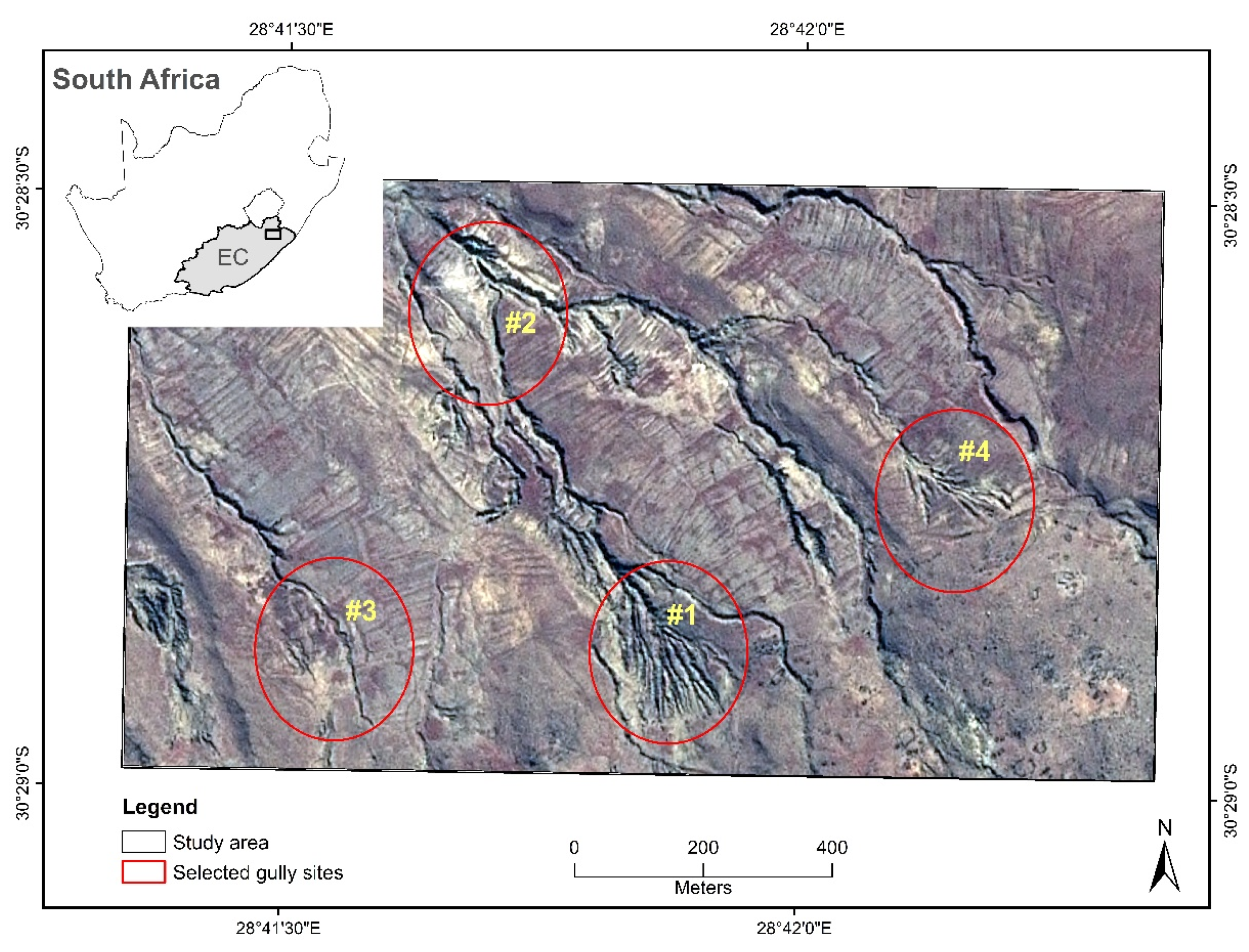
2.1. Study Area

Approximately 70% of South African land is classified as degraded, with the Eastern Cape (EC) Province being the province most endangered by water erosion [35]. Our study area (1.47 km2) is located in the EC province and is one the erosion hotspots in the province (Figure 1). The most common type of water erosion occurring within the study area is gully erosion, particularly permanent gullies. These permanent gullies have varying lengths (30–274 m), depths (1.22–6.90 m), widths (4.66–15 m) and appearances (narrow, elongated, short, wide, linear) and are distributed across agricultural lands. These differences in appearance can be readily observed in four selected gully sites (#1–#4). Gullies in sites #1 and #4 share almost the same appearance/pattern (i.e., dense network of gullies forming a dendritic-like pattern) but generally differ in depth, i.e., steep-sided gullies (with shadows) are more frequent in site #1 than in site #4. In sites #2 and #3, gullies are mostly of linear pattern and elongated. The longest gully is located within site #3, whereas the deepest and widest gullies occur in site #2. The climate of the study area is semiarid with temperatures ranging from 7 °C to 30 °C and an annual rainfall of approximately 670 mm. The elevation ranges from 1445 m to 1584 m and the highest elevation values correspond to the western parts, whereas the lowest values are found in the far southeastern parts of the study area. The land use is predominately agriculture (crop and livestock farming). Heavily grazed by livestock, vegetation mainly consists of Highland Sourveld Grassland [36], occurring in hilly and mountainous parts of the area. Most agricultural areas are located on gentle sloping lands dissected by continuous and discontinuous gullies. Gully erosion in this area is driven by a host of factors, mainly anthropogenic-based, relating to unsustainable land use and inappropriate agricultural practices [37,38]. Shallow and potentially erodible soils of Mispath and Glenrose soil forms [39], and the prevalence of subsurface (piping) erosion also predispose the area to gully erosion [40]. The geology of the area is predominantly mudstone and sandstone of the Beaufort Group [41].

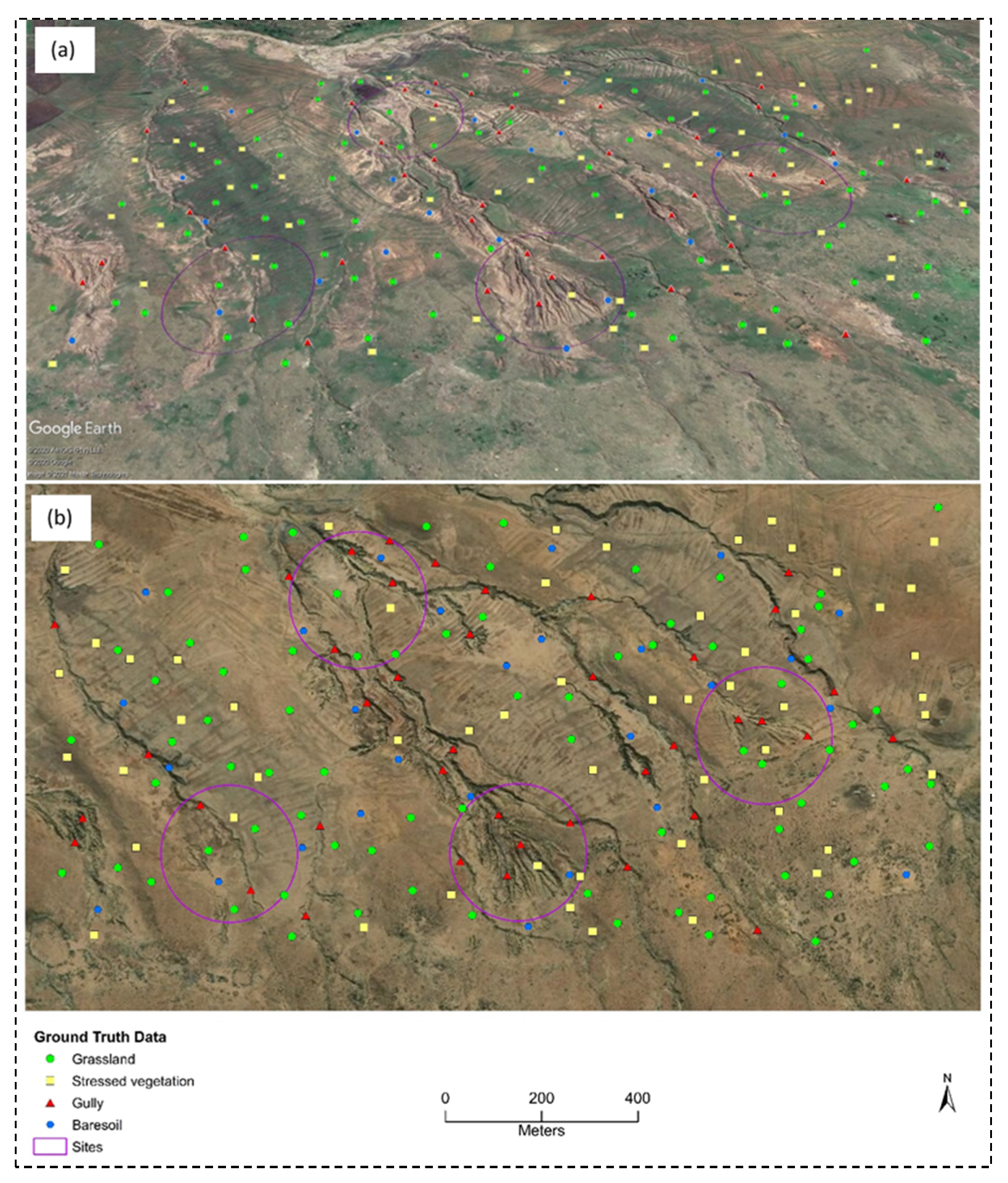
2.2. Data and Pre-Processing

The data set used consisted of a cloud-free Systeme Pour l’Observation de la Terre (SPOT-7) RGB (Red, Green, Blue) image acquired on 25 June 2017. The image was acquired from the South African National Space Agency (SANSA) and had already been orthorectified and pan-sharpened to 1.3 m spatial geometric resolution by the supplier. Reflectance values were obtained using the Apparent Reflectance module in ArcGIS. A 30 m Shuttle Radar Topography Mission (SRTM) digital elevation model (DEM) was downloaded on 26 January 2021 from Earth Explorer website (https://earthexplorer.usgs.gov/).

2.3. Classification and Accuracy Assessment

We identified four land cover classes: grassland (GL), stressed vegetation (SV), gully (G), and bare soil (BS). High resolution Google Earth images together with aerial images available in ArcGIS Online were used to collect ground truth data (Figure 2). Using random sampling, we collected 200 points for four land cover classes: GL (78), SV (54), G (41), and BS (27). The points were prepared in ArcGIS and later exported to Google Earth. Image classification was performed on 10 October 2020 in the Sentinels Application Platform (SNAP) software (http://step.esa.int) using four classifiers, including k-dimensional tree K-Nearest Neighbor (k-d tree KNN), Minimum Distance (MD), Maximum Likelihood (ML), and Random Forest (RF). A description of each classifier is summarized in Table 1. Although this study focused on mapping gullies, involving other land cover categories in the classification was necessary for discriminating gullies from the surrounding land cover. Also, the SNAP software required four land cover categories as minimum input training data. Although the Normalized Green Red Difference Index (NGRDI) was not involved directly in the classification, we computed it to gain insight on vegetation distribution in relation to gullied areas. We calculated the NGRDI in ArcMap based on the formula: (G − R)/(G + R), where G is the Green band and R is the Red band. We extracted the NGRDI spectral profiles of gullies based on gully transects ranging from 20 m to 100 m in length using ENVI 5.3.
In order to obtain a gully map, we reclassified the land cover map into binary level (gully and non-gully class). This gully map was clipped into four selected gully sites to further investigate the influence of gully characteristics, i.e., shape, size, length, width, and depth. We manually digitized gullies based on high resolution (0.5 m) aerial photography for each of the selected four sites. Digitization was carried out in ArcMap at a scale of 1:500. The digitized polygons were then converted to raster format. These manually digitized gullies were used to check how well automatically extracted gullies compare to the actual extent of gullies.
The accuracy of the automatic classification was assessed using the confusion matrix [46,47], a widely used method that provides various accuracy metrics such as the overall accuracy (OA), kappa coefficient, user’s accuracy (UA), and producer’s accuracy (PA). OA refers to a ratio of correctly classified pixels. OA is computed by dividing the sum of correctly classified pixels by the sum of reference pixels. PA is calculated by dividing the number of correctly classified pixels in each class by the column total representing reference data. UA is calculated like PA except that the row total representing predicted classes is used to divide the number of correctly classified pixels. PA indicates how well reference pixels of the ground cover type represent the classified class, while UA represents the probability that a given pixel was classified into the class that actually represents it on the ground.
The gully density map was computed to visualize the intensity or severity of gullies across the study area. We computed the gully density map in ArcGIS software using the Line Density tool. We calculated the lengths of the gullies and determined their density per unit area. We chose RF-classified gullies since the algorithm provided good gully classification results. We chose meters as a unit of measure for both length and area, i.e., gully length (m)/m2. Input data were the gully map (RF classification) having the best overall and class-level accuracies.

3. Results

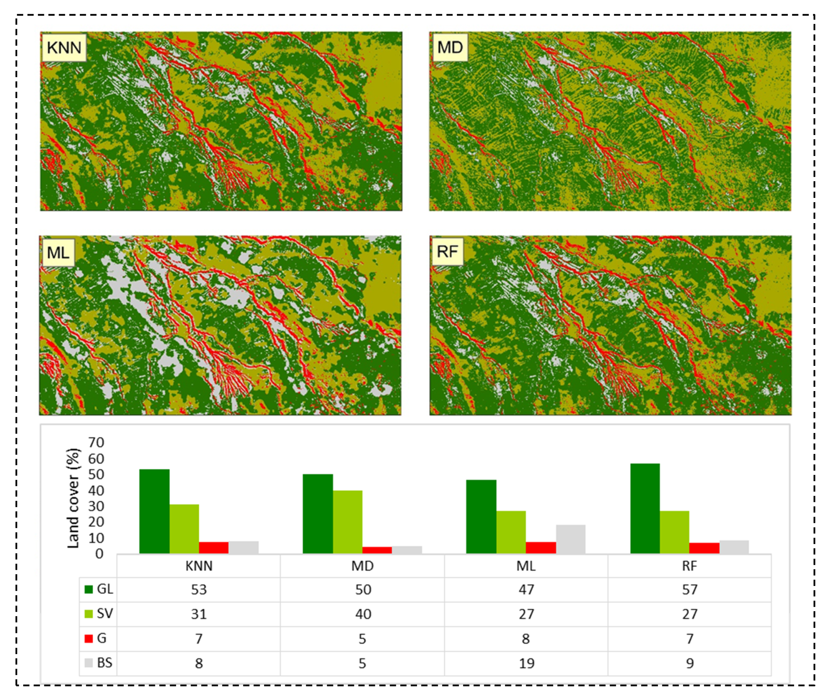
3.1. Land Cover Distribution

Different classifiers resulted in varying outcomes in terms of land cover classification (Figure 3). In all classifiers, grassland (GL) contributed the largest proportion (47–57%) of land cover, followed by the stressed vegetation (SV) class ranging from 27–31%. The gully (G) class (5–8%) was the least land cover and the bare soil (BS) class (5%) in the case of the MD classifier. Of all classifiers, the ML recorded the highest BS (19%) and G (8%) whereas RF and KNN accounted for the largest proportions of GL (57%) and SV (31%) classes, respectively. In contrast, the MD classifier had the lowest coverage (5%) in terms of gully classification.

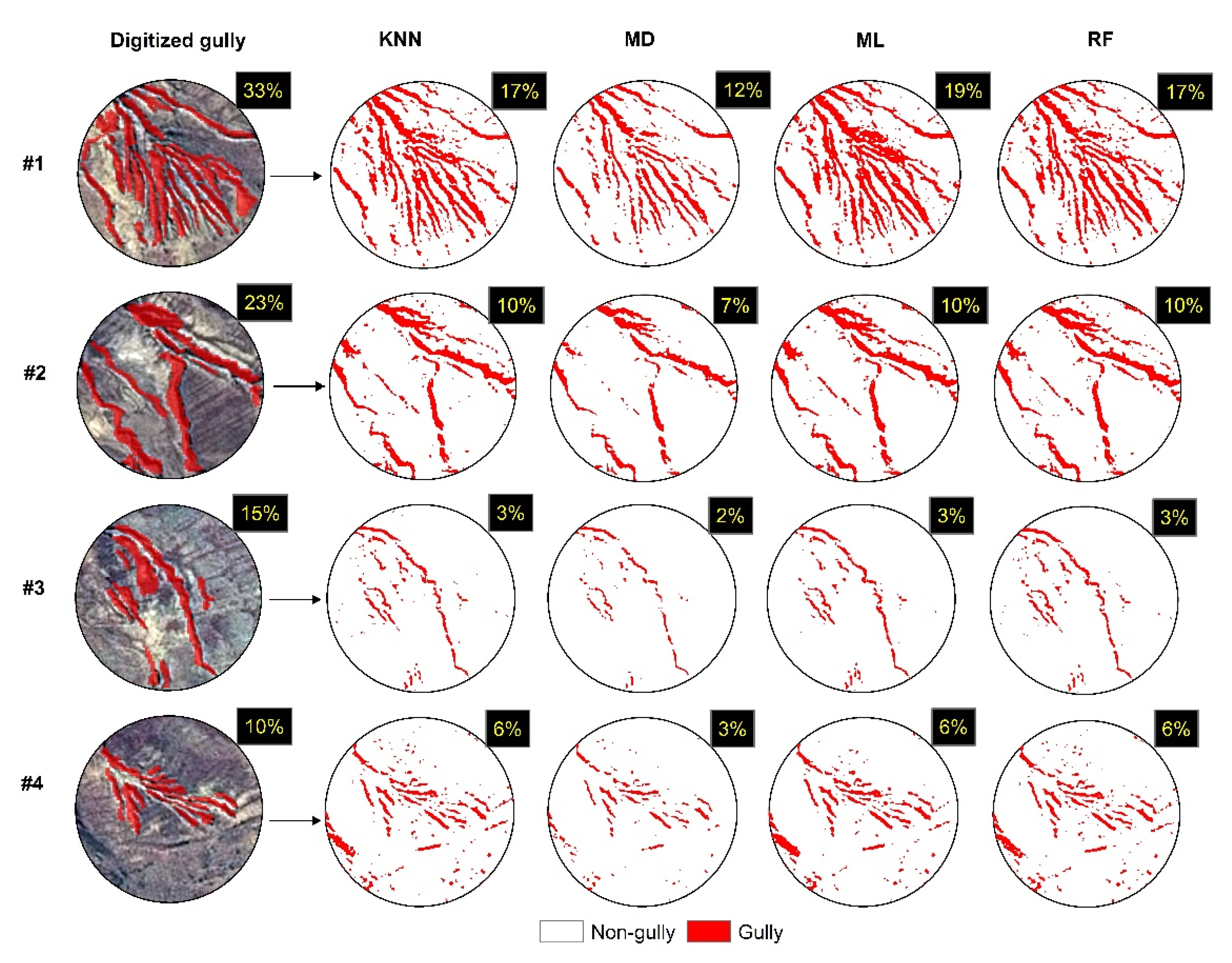
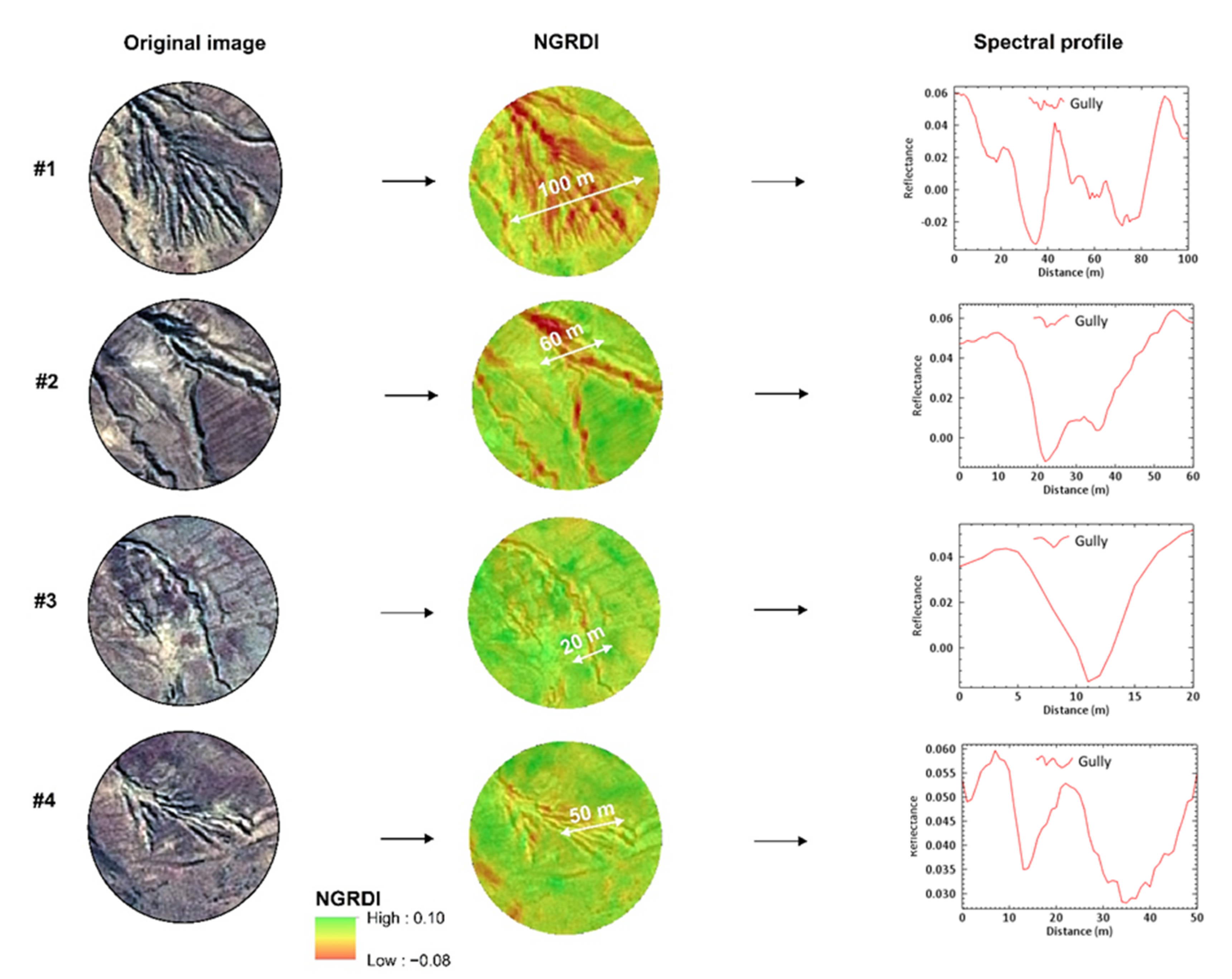
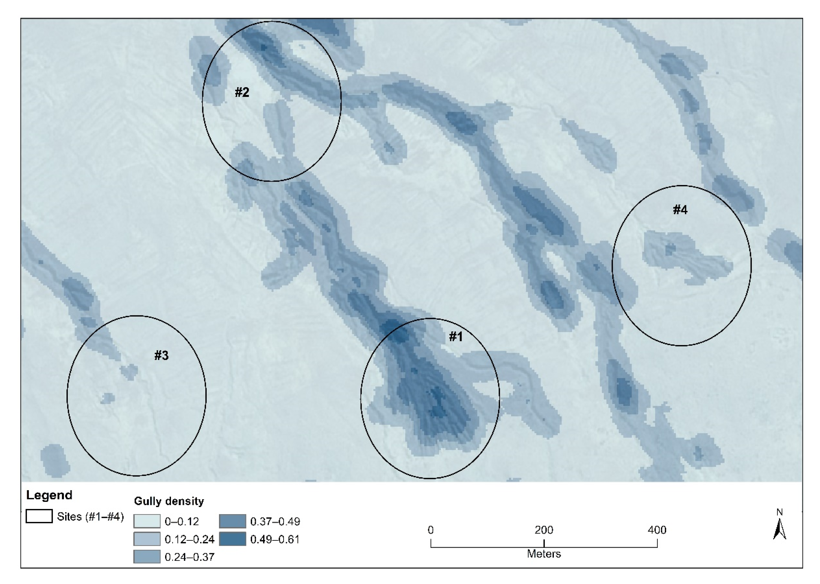
3.2. Gully Distribution in Selected Sites

Generally, site #1 had the largest proportion of gullied area although different classifiers had varied results, lying within the range of 12–19% (9321–10344 m2; Figure 4, Table 2). Sites #3 and #4 were the least gullied sites with a spatial extent of 1668 m2 to 3147 m2 (3–6%) for the latter and 1039 m2 to 1774 m2 (2–3%) for the former. In all selected gully sites, the MD classifier consistently obtained the least gully area. Other classifiers recorded the same results in four selected sites with the exception of site #1 where the ML had the highest areal extent of gully erosion (19%), followed by RF and KNN both recording 17%, and then MD (12%).
Different algorithms did not differ relevantly regarding the classified gullies from the actual (digitized) gullies, at least in terms of their spatial distribution patterns, but there was a clear lack of agreement in the proportion of areas classified as gullies. In all sites, the algorithms missed gullies by a considerable amount, and the most remarkable difference was at site #3, where KNN, ML and RF classified 1774 m2 as gullied area whereas MD only resulted in 1039 m2, compared to the actual gullied area (8064 m2).

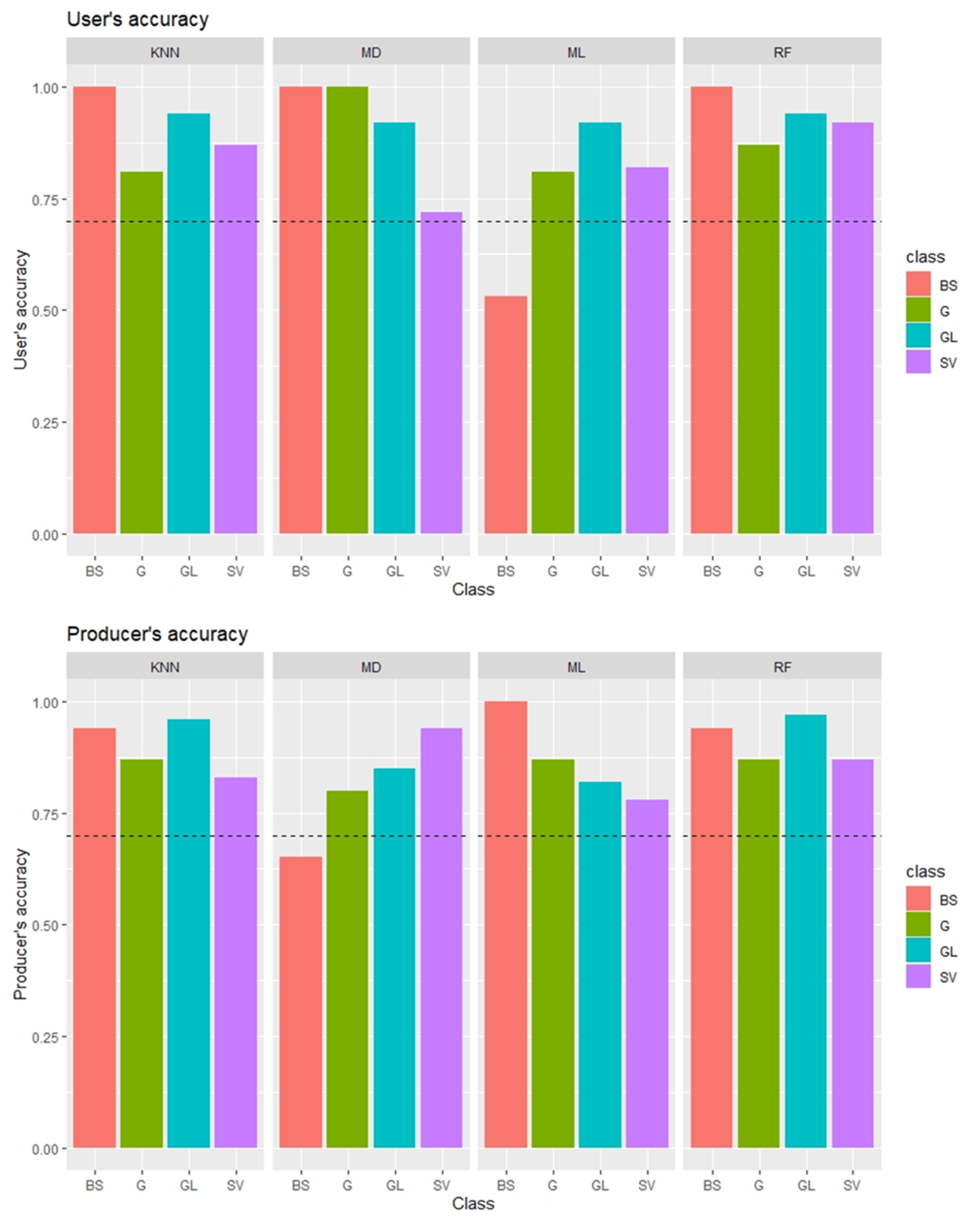
3.3. Overall and Class-Level Accuracies

All classifiers recorded overall accuracies above 0.80. The ML classifier obtained the lowest OA (0.83) and kappa (0.72), while RF (0.94) had the highest OA and kappa (0.89), followed by KNN, which recorded 0.92 (OA) and 0.86 (kappa), and then MD, which obtained 0.86 (OA) and 0.76 (kappa). Results revealed considerable differences in user’s accuracy (UA) and producer’s accuracy (PA) obtained by various classifiers (Figure 5). Generally, KNN, MD and RF showed exceptional performance in classifying BS class, all recording 1.00 (100%) UA. In contrast, the ML classifier achieved a relatively low UA (0.60), but had the highest PA (100%) relative to other classifiers. MD outperformed other classifiers in gully (G) classification with 100% UA, although the corresponding PA was only 0.80. RF achieved the highest OA (0.94), UA was only 87% in classifying gullies.

4. Discussion

4.1. SPOT-7 RGB Bands and Gully Extraction

Results showed that the SPOT-7 image, even with limited spectral information (e.g., RGB), can effectively help to discriminate gullies from other land cover types, which is in line with findings of previous research [18]. The absence of near-infrared (NIR) band did not have a direct bearing on gully classification as the spatial resolution was sufficiently high (1.3 m) to detect most gullies. NGRDI proved that gullies can be discriminated from vegetation and other surrounding land cover classes (Figure 6). This is evident in both the NGRDI map and the corresponding spectral profiles of gullies: a typical V-shaped gully morphology in site #3 is apparent in the spectral profile. Dendritic network of gullies in sites #1 and #4, typified by a series of V-shapes, are also evident in the corresponding spectral profiles. However, the absence of the near-infrared (NIR) band presented a challenge in vegetation identification during the training data selection stage. This challenge was exacerbated by the fact that the image was acquired during the dry season, making it difficult to visually identify vegetation, particularly sparse and short vegetation cover. The use of high resolution Google Earth images of the same month as the SPOT image helped in the identification of vegetation cover during the training phase.

4.2. Efficacy of Machine Learnining Algorithms

Usually, an overall accuracy (OA) rates of at least 0.85 and 0.70 for class-specific accuracies, i.e., producer’s accuracy (PA) and user’s accuracy (UA), are recommended as a benchmark accuracy for operational purposes [48]. Excepting the ML classifier, which had the lowest OA (0.83), all other classifiers crossed the 0.85 benchmark, with RF (0.94) and KNN (0.92) recording above 0.90, whereas MD had an OA of 0.86. The higher performance of RF compared to other methods was not surprising; similar findings have been reported [49]. Although different classifiers have different advantages over one another, the RF classifier, as an ensemble learning algorithm, appears to be more advantageous than other classifiers for a number of reasons. The idea behind classifier ensembles is based upon the basic premise that a set of classifiers do perform better classifications than an individual classifier does [50].
While OA is one of the most widely used metrics with easy interpretation and practical value [23], an important setback is that it hides class-specific performance [51]. Considering 0.70 class-level accuracy benchmark, the algorithms successfully classified gullies, recording PAs and UAs above the benchmark. It is also worth noting that the classification of a relatively large gully area does not equate to higher accuracies. This is especially true with respect to the MD classifier which, of all classifiers, obtained the smallest proportion of gully area in all four selected sites (Figure 4), but had no commission error (e.g., 100% UA) and obtained 20% omission error. KNN and ML had the same commission (19%) and omission (13%) errors, while RF recorded 13% in both omission and commission errors. In general, these errors are relatively low, compared to those of previous studies conducted in South Africa [14,16,52]. However, it is worth exploring and understanding possible sources of these errors relevant to this study.
The different characteristics of gullies had a strong bearing on gully classification. Results showed that classifiers were most efficient in areas where gullies took a dendritic pattern, like site #1. However, in site #4, which was also characterized by a network of dendritic gullies like site #1, classifiers were not efficient in detecting gullies. This may be because gullies are a bit shallow in site #4 compared to site #1. The deepest and widest gullies occurred in site #2. Depth (present of shadows) appeared to be more important in gully discrimination than width. Wider and shallow-sided gullies were difficult to detect especially if they occurred on bare soil. Length of the gully was not that important when it came to gully detection. Site #3 had the longest gully, but because of the shallow gully walls, classifiers were less efficient. Results showed a discrepancy between the actual (digitized) gullies and those derived by the algorithms in all sites. There are two possible reasons for such a discrepancy. First, the classifiers mostly detected gullies with steep-sided walls (or at least with some shadows), whereas digitized gullies were captured in their correct shape with exact boundaries. Second, differences in resolutions between the aerial photograph (0.5 m) used to digitize gullies and SPOT (1.3 m) used to classify gullies might have contributed to the observed discrepancy. Similar findings were reported in another study [53], where the pixel resolution of the chosen input data was not fine enough to sufficiently capture the flat parts of the gullies, leading to under-classification of gullies.

4.3. Gully Density Map

Gullies represent a serious threat to sustainable agriculture, potentially undermining food security, particularly in developing countries. Gullies change spatially and temporally, requiring continuous mapping and monitoring, hence, the need for suitable automatic methods for gully erosion assessment. A gully density map can be an important index for gully severity evaluation. The gully density for this study ranged from 0.12 m/m2 to 0.61 m/m2 (Figure 7). We found that different appearances/pattern of gullies exhibited different gully densities. For example, site #1, dissected by a dendritic network of gullies, had the highest gully density. This was exacerbated by lack of vegetation cover in between the dense network of gullies. Linear and V-shaped gullies with steep-sided walls in site #2 also appeared to have high density, although this varied across the study area. Other studies found that the slope steepness plays an important role in gully density. For instance, Zhang et al. [54] reported a significant positive correlation between slope gradient and gully density on the hillslope. Similarly, Munoz-Robles et al. [55] found that most parts of their study area with gullies had steeper slopes. Although the topography of this study had some hilly areas, the studied gullies were distributed on gentle sloping agricultural land, thus, slope was not the overriding factor.
The findings presented in this study can be a useful source of information regarding the location of vulnerable agricultural areas, thereby assisting decision makers and land managers in combating soil erosion. In South Africa, the need to map gullies using remote sensing data was identified [56], and many researchers have since heeded the call [16,29,57]. SPOT images proved to be effective in gully mapping [18], even at a national scale [29]. However, multi-date and multi-season SPOT images, which were not available in the present study, can be particularly important in monitoring gullies. Further research should focus on testing RF, KNN, ML and MD classifiers on images acquired in different seasons. In our study, these algorithms were applied with their default parameters, fine tuning parameters could improve the classification outcome.

5. Conclusions

The selection of an appropriate classifier is a critical step in remote sensing of land cover, particularly gully erosion. This study examined four (KNN, MD, ML, and RF) well known but different classifiers (parametric and non-parametric) in mapping permanent gullies within an agricultural area. Key conclusions were as follows:
  • Different characteristics of gullies, most notably, shape/pattern (e.g., dendritic) and depth, had a strong bearing on gully classification;
  • No single classifier outperformed other classifiers in all accuracy metrics (e.g., OA, UA, and PA);
  • All classifiers except ML had OA values that exceeded the 0.85 benchmark. RF showed the best performance regarding the OA (i.e., 0.94);
  • MD was the most effective classifier in gully mapping based on UA (100%) but obtained the lowest PA (0.80), while KNN, ML, and RF classifiers equally recorded a PA value of 0.87;
  • Despite the differences in UA and PA values, all classifiers crossed the 0.70 class-specific benchmark for gullies, but RF outperformed the other algorithms regarding the class-level accuracy metrics (UA and PA);
  • Remote sensing, with the aid of appropriate machine learning algorithms, is a useful tool for gully density mapping;
  • Although there are limitations to the usage of satellite images, this approach works well if there is no vegetation inside the gullies. Thus, the approach is suitable for arid/semiarid regions.

Author Contributions

Conceptualization, K.P. and S.S.; methodology, K.P. and S.S.; software, K.P. and S.S.; validation, K.P. and I.H.; formal analysis, I.H.; investigation, K.P., S.S. and I.H.; resources, I.H. and S.S.; data curation, K.P. and S.S.; writing—original draft preparation, K.P., S.S. and I.H.; visualization, K.P.; supervision, S.S.; project administration, I.H.; funding acquisition, I.H. All authors have read and agreed to the published version of the manuscript.

Funding

The research was supported by the TNN 123457 NKFI, K131478 and the Thematic Excellence Programme (TKP2020-NKA-04) of the Ministry for Innovation and Technology in Hungary projects.

Institutional Review Board Statement

Not applicable.

Informed Consent Statement

Not applicable.

Data Availability Statement

The data presented in this study are available on request from the corresponding author.

Acknowledgments

We thank the South African National Space Agency (SANSA) for providing the free SPOT-7 image. The first author is indebted to the Tempus Public Foundation (Hungary) for funding his Ph.D. studies through the Stipendium Hungaricum Scholarship Program, supported by the Department of Higher Education and Training (DHET) of South Africa.

Conflicts of Interest

The authors declare no conflict of interest. The funders had no role in the design of the study; in the collection, analyses, or interpretation of data; in the writing of the manuscript, or in the decision to publish the results.

References

  1. Shi, Z.H.; Fang, N.F.; Wu, F.Z.; Wang, L.; Yue, B.J.; Wu, G.L. Soil Erosion Processes and Sediment Sorting Associated with Transport Mechanisms On Steep Slopes. J. Hydrol. 2012, 454, 123–130. [Google Scholar] [CrossRef]
  2. Lal, R. Soil Degradation by Erosion. Land Degrad. Dev. 2001, 12, 519–539. [Google Scholar] [CrossRef]
  3. Pimentel, D. Soil Erosion: A Food and Environmental Threat. Environ. Dev. Sustain. 2006, 8, 119–137. [Google Scholar] [CrossRef]
  4. Food and Agriculture Organization of the United Nations. Soil Erosion: The Greatest Challenge for Sustainable Soil Management; FAO: Rome, Italy, 2019; ISBN 9780511807527. [Google Scholar]
  5. Kosmas, C.; Danalatos, N.; Cammeraat, L.H.; Chabart, M.; Diamantopoulos, J.; Farand, R.; Gutierrez, L.; Jacob, A.; Marques, H.; Martinez-Fernandez, J. The Effect of Land Use on Runoff and Soil Erosion Rates under Mediterranean Conditions. Catena 1997, 29, 45–59. [Google Scholar] [CrossRef]
  6. Blake, W.H.; Rabinovich, A.; Wynants, M.; Kelly, C.; Nasseri, M.; Ngondya, I.; Patrick, A.; Mtei, K.; Munishi, L.; Boeckx, P.; et al. Soil Erosion in East Africa: An Interdisciplinary Approach to Realising Pastoral Land Management Change. Environ. Res. Lett. 2018, 13. [Google Scholar] [CrossRef] [Green Version]
  7. Drees, L.R.; Wilding, L.P.; Owens, P.R.; Wu, B.; Perotto, H.; Sierra, H. Steepland Resources: Characteristics, Stability and Micromorphology. Catena 2003, 54, 619–636. [Google Scholar] [CrossRef]
  8. Phinzi, K.; Ngetar, N.S. The Assessment of Water-Borne Erosion at Catchment Level Using GIS-Based RUSLE and Remote Sensing: A Review. Int. Soil Water Conserv. Res. 2019, 7, 27–46. [Google Scholar] [CrossRef]
  9. Phinzi, K.; Ngetar, N.S.; Ebhuoma, O. Soil Erosion Risk Assessment in the Umzintlava Catchment (T32E), Eastern Cape, South Africa, Using RUSLE and Random Forest Algorithm. S. Afr. Geogr. J. 2020, 1–24. [Google Scholar] [CrossRef]
  10. Mohammed, S.; Al-Ebraheem, A.; Holb, I.J.; Alsafadi, K.; Dikkeh, M.; Pham, Q.B.; Linh, N.T.T.; Szabo, S. Soil Management Effects on Soil Water Erosion and Runoff in Central Syria—A Comparative Evaluation of General Linear Model and Random Forest Regression. Water 2020, 12, 2529. [Google Scholar] [CrossRef]
  11. Wischmeier, W.H.; Smith, D.D. Predicting Rainfall Erosion Losses: A Guide to Conservation Planning; Department of Agriculture, Science and Education Administration: Beltsville, MD, USA, 1978. [Google Scholar]
  12. Poesen, J.; Nachtergaele, J.; Verstraeten, G.; Valentin, C. Gully Erosion and Environmental Change: Importance and Research Needs. Catena 2003, 50, 91–133. [Google Scholar] [CrossRef]
  13. Bertalan, L.; Túri, Z.; Szabó, G. UAS Photogrammetry and Object-Based Image Analysis (Geobia): Erosion Monitoring at the Kazár badland, Hungary. Landsc. Environ. 2016, 10, 169–178. [Google Scholar] [CrossRef] [Green Version]
  14. Phinzi, K.; Ngetar, N.S. Mapping Soil Erosion in a Quaternary Catchment in Eastern Cape Using Geographic Information System and Remote Sensing. S. Afr. J. Geomat. 2017, 6, 11. [Google Scholar] [CrossRef] [Green Version]
  15. Bui, D.T.; Shirzadi, A.; Shahabi, H.; Chapi, K.; Omidavr, E.; Pham, B.T.; Asl, D.T.; Khaledian, H.; Pradhan, B.; Panahi, M.; et al. A Novel Ensemble Artificial Intelligence Approach for Gully Erosion Mapping in a Semi-Arid Watershed (Iran). Sens. Switz. 2019, 19, 2444. [Google Scholar] [CrossRef] [Green Version]
  16. Makaya, N.P.; Mutanga, O.; Kiala, Z.; Dube, T.; Seutloali, K.E. Assessing the Potential of Sentinel-2 MSI Sensor in Detecting and Mapping the Spatial Distribution of Gullies in a Communal Grazing Landscape. Phys. Chem. Earth 2019, 112, 66–74. [Google Scholar] [CrossRef]
  17. Karydas, C.; Panagos, P. Towards an Assessment of the Ephemeral Gully Erosion Potential in Greece Using Google Earth. Water 2020, 12, 603. [Google Scholar] [CrossRef] [Green Version]
  18. Phinzi, K.; Abriha, D.; Bertalan, L.; Holb, I.; Szabó, S. Machine Learning for Gully Feature Extraction Based on a Pan-Sharpened Multispectral Image: Multiclass vs. Binary Approach. ISPRS Int. J. Geo Inf. 2020, 9, 252. [Google Scholar] [CrossRef] [Green Version]
  19. Zhang, L.; Zhang, L.; Du, B. Deep Learning for Remote Sensing Data: A Technical Tutorial on the State of the Art. IEEE Geosci. Remote Sens. Mag. 2016, 4, 22–40. [Google Scholar] [CrossRef]
  20. LeCun, Y.; Bottou, L.; Bengio, Y.; Haffner, P. Gradient-Based Learning Applied to Document Recognition. Proc. IEEE 1998, 86, 2278–2324. [Google Scholar] [CrossRef] [Green Version]
  21. Chen, G.; Zhang, X.; Wang, Q.; Dai, F.; Gong, Y.; Zhu, K. Symmetrical Dense-Shortcut Deep Fully Convolutional Networks for Semantic Segmentation of Very-High-Resolution Remote Sensing Images. IEEE J. Sel. Top. Appl. Earth Obs. Remote Sens. 2018, 11, 1633–1644. [Google Scholar] [CrossRef]
  22. Ma, L.; Liu, Y.; Zhang, X.; Ye, Y.; Yin, G.; Johnson, B.A. Deep Learning in Remote Sensing Applications: A Meta-Analysis and Review. ISPRS J. Photogramm. Remote Sens. 2019, 152, 166–177. [Google Scholar] [CrossRef]
  23. Heydari, S.S.; Mountrakis, G. Effect of Classifier Selection, Reference Sample Size, Reference Class Distribution and Scene Heterogeneity in Per-Pixel Classification Accuracy Using 26 Landsat Sites. Remote Sens. Environ. 2018, 204, 648–658. [Google Scholar] [CrossRef]
  24. Ge, W.; Cheng, Q.; Tang, Y.; Jing, L.; Gao, C. Lithological Classification Using Sentinel-2A Data in the Shibanjing Ophiolite Complex in Inner Mongolia, China. Remote Sens. 2018, 10, 638. [Google Scholar] [CrossRef] [Green Version]
  25. Szabó, S.; Burai, P.; Kovács, Z.; Szabó, G.; Kerényi, A.; Fazekas, I.; Paládi, M.; Buday, T.; Szabó, G. Testing Algorithms for the Identification of Asbestos Roofing Based on Hyperspectral Data. Environ. Eng. Manag. J. 2014, 143, 2875–2880. [Google Scholar] [CrossRef]
  26. Lu, D.; Weng, Q. A Survey of Image Classification Methods and Techniques for Improving Classification Performance. Int. J. Remote Sens. 2007, 28, 823–870. [Google Scholar] [CrossRef]
  27. Fadul, H.M.; Salih, A.A.; Ali, I.E.A.; Inanaga, S. Use of Remote Sensing to Map Gully Erosion along the Atbara River, Sudan. Int. J. Appl. Earth Obs. Geoinf. 1999, 1999, 175–180. [Google Scholar] [CrossRef]
  28. Daba, S.; Rieger, W.; Strauss, P. Assessment of Gully Erosion in Eastern Ethiopia Using Photogrammetric Techniques. Catena 2003, 50, 273–291. [Google Scholar] [CrossRef]
  29. Mararakanye, N.; Le Roux, J.J. Gully Location Mapping at a National Scale for South Africa. S. Afr. Geogr. J. 2012, 94, 208–218. [Google Scholar] [CrossRef]
  30. Fiorucci, F.; Ardizzone, F.; Rossi, M.; Torri, D. The Use of Stereoscopic Satellite Images to Map Rills and Ephemeral Gullies. Remote Sens. 2015, 7, 14151–14178. [Google Scholar] [CrossRef] [Green Version]
  31. James, L.A.; Watson, D.G.; Hansen, W.F. Using LiDAR Data to Map Gullies and Headwater Streams under Forest Canopy: South Carolina, USA. Catena 2007, 71, 132–144. [Google Scholar] [CrossRef]
  32. Korzeniowska, K.; Pfeifer, N.; Landtwing, S. Mapping Gullies, Dunes, Lava Fields, and Landslides via Surface Roughness. Geomorphology 2018, 301, 53–67. [Google Scholar] [CrossRef]
  33. Rijal, S.; Wang, G.; Woodford, P.B.; Howard, H.R.; Hutchinson, J.M.S.; Hutchinson, S.; Schoof, J.; Oyana, T.J.; Li, R.; Park, L.O. Detection of Gullies in Fort Riley Military Installation Using LiDAR Derived High Resolution DEM. J. Terramech. 2018, 77, 15–22. [Google Scholar] [CrossRef]
  34. Đomlija, P.; Gazibara, S.B.; Arbanas, Ž.; Arbanas, S.M. Identification and Mapping of Soil Erosion Processes Using the Visual Interpretation of Lidar Imagery. ISPRS Int. J. Geo Inf. 2019, 8, 438. [Google Scholar] [CrossRef] [Green Version]
  35. Garland, G.G.; Hoffman, M.T.; Todd, S. Soil Degradation. In A National Review of Land Degradation in South Africa, Hoffman, M.T., Todd, S., Ntshona, Z., Turner, S., Eds.; South African National Biodiversity Institute: Pretoria, South Africa, 2000; pp. 69–107. [Google Scholar]
  36. Acocks, J.P.H. Veld types of South Africa; BRIT Press: Fort Worth, TX, USA, 1988; ISBN 0621113948. [Google Scholar]
  37. Kakembo, V.; Rowntree, K.M. The Relationship between Land Use and Soil Erosion in the Communal Lands near Peddie Town, Eastern Cape, South Africa. L. Degrad. Dev. 2003, 14, 39–49. [Google Scholar] [CrossRef]
  38. Phinzi, K.; Ngetar, N.S. Land Use/Land Cover Dynamics and Soil Erosion in the Umzintlava Catchment (T32E), Eastern Cape, South Africa. Trans. R. Soc. S. Afr. 2019, 74, 223–237. [Google Scholar] [CrossRef]
  39. van Breda Weaver, A. The Distribution of Soil Erosion as a Function of Slope Aspect and Parent Material in Ciskei, Southern Africa. GeoJournal 1991, 23, 29–34. [Google Scholar] [CrossRef]
  40. Beckedahl, H.R.; de Villiers, A.B. Accelerated Erosion by Piping in the Eastern Cape Province, South Africa. S. Afr. Geogr. J. 2000, 82, 157–162. [Google Scholar] [CrossRef]
  41. Hilbich, C.; Daut, G.; Mäusbacher, R.; Helmschrot, J. A Landscape-Based Model to Characterize the Evolution and Recent Dynamics of Wetlands in the Umzimvubu Headwaters, Eastern Cape, South Africa; Okruszko, T., Maltby, E., Szatylowicz, J., Miroslaw-Swiatek, D., Eds.; Taylor & Francis Group: Oxfordshire, UK, 2007; p. 61. ISBN 978-0-415-40820-2. [Google Scholar]
  42. Thanh Noi, P.; Kappas, M. Comparison of Random Forest, K-Nearest Neighbor, and Support Vector Machine Classifiers for Land Cover Classification Using Sentinel-2 Imagery. Sens. Basel 2017, 18, 18. [Google Scholar] [CrossRef] [PubMed] [Green Version]
  43. Richards, J.A.; Richards, J.A. Remote Sensing Digital Image Analysis; Springer: New York, NY, USA, 1999; Volume 3, ISBN 3642300618. [Google Scholar]
  44. Bolstad, P.V.; Lillesand, T.M. Rapid Maximum Likelihood Classification. Photogramm. Eng. Remote Sens. 1991, 57, 67–74. [Google Scholar]
  45. Breiman, L. Random Forests. Mach. Learn. 2001, 45, 5–32. [Google Scholar] [CrossRef] [Green Version]
  46. Congalton, R.G. A Review of Assessing the Accuracy of Classifications of Remotely Sensed Data. Remote Sens. Environ. 1991, 37, 35–46. [Google Scholar] [CrossRef]
  47. Congalton, R.G.; Green, K. Assessing the Accuracy of Remotely Sensed Data: Principles and Practices; CRC Press: Boca Raton, FL, USA, 2019; ISBN 0429629354. [Google Scholar]
  48. Everitt, J.H.; Yang, C.; Fletcher, R.; Deloach, C.J. Comparison of QuickBird and SPOT 5 Satellite Imagery for Mapping Giant Reed. J. Aquat. Plant Manag. 2008, 46, 77–82. [Google Scholar]
  49. Khatami, R.; Mountrakis, G.; Stehman, S.V. A Meta-Analysis of Remote Sensing Research on Supervised Pixel-Based Land-Cover Image Classification Processes: General Guidelines for Practitioners and Future Research. Remote Sens. Environ. 2016, 177, 89–100. [Google Scholar] [CrossRef] [Green Version]
  50. Rodriguez-Galiano, V.F.; Ghimire, B.; Rogan, J.; Chica-Olmo, M.; Rigol-Sanchez, J.P. An Assessment of the Effectiveness of a Random Forest Classifier for Land-Cover Classification. ISPRS J. Photogramm. Remote Sens. 2012, 67, 93–104. [Google Scholar] [CrossRef]
  51. He, H.; Garcia, E.A. Learning from Imbalanced Data. IEEE Trans. Knowl. Data Eng. 2009, 21, 1263–1284. [Google Scholar]
  52. Mararakanye, N.; Nethengwe, N.S. Gully Erosion Mapping Using Remote Sensing Techniques. S. Afr. J. Geomat. 2012, 1, 109–118. [Google Scholar]
  53. d’Oleire-Oltmanns, S.; Marzolff, I.; Tiede, D.; Blaschke, T. Detection of Gully-Affected Areas by Applying Object-Based Image Analysis (OBIA) in the Region of Taroudannt, Morocco. Remote Sens. 2014, 6, 8287–8309. [Google Scholar] [CrossRef] [Green Version]
  54. Zhang, T.; Liu, G.; Duan, X.; Wilson, G.V. Spatial Distribution and Morphologic Characteristics of Gullies in the Black Soil Region of Northeast China: Hebei Watershed. Phys. Geogr. 2016, 37, 228–250. [Google Scholar] [CrossRef]
  55. Muñoz-Robles, C.; Reid, N.; Frazier, P.; Tighe, M.; Briggs, S.V.; Wilson, B. Factors Related to Gully Erosion in Woody Encroachment in South-Eastern Australia. Catena 2010, 83, 148–157. [Google Scholar] [CrossRef]
  56. Le Roux, J.J.; Newby, T.S.; Sumner, P.D. Monitoring Soil Erosion in South Africa at a Regional Scale: Review and Recommendations. S. Afr. J. Sci. 2007, 103, 329–335. [Google Scholar]
  57. Phinzi, K.; Ngetar, N.S.; Ebhuoma, O.; Szabó, S. Comparison of Rusle and Supervised Classification Algorithms for Identifying Erosion-Prone Areas in a Mountainous Rural Landscape. Carpathian J. Earth Environ. Sci. 2020, 15. [Google Scholar] [CrossRef]
Figure 1. Location of study area, Eastern Cape (EC), South Africa. Selected gully sites (#1–#4).
Agronomy 11 00333 g001
Figure 2. Ground truth points distributed across the study area: (a) Google Earth and (b) aerial photograph (ArcGIS Online).
Agronomy 11 00333 g002
Figure 3. Land cover classification (GL: grassland, SV: stressed vegetation, G: gully, BS: bare soil) based on different algorithms (KNN: k-nearest neighbor, MD: minimum distance, ML: maximum likelihood, RF: random forest).
Agronomy 11 00333 g003
Figure 4. Selected gully sites (1–4) showing the spatial distribution of the classified gullies by different algorithms (KNN: k-nearest neighbor, MD: minimum distance, ML: maximum likelihood, RF: random forest) and actual (digitized) gullies.
Agronomy 11 00333 g004
Figure 5. User’s accuracy and producer’s accuracy (dashed black line indicates class accuracy benchmark of 0.70; GL: grassland, SV: stressed vegetation, G: gully, BS: bare soil).
Agronomy 11 00333 g005
Figure 6. Gully transects (20–100 m) with Normalized Green Red Difference Index (NGRDI)-based spectral profiles of selected gullies.
Agronomy 11 00333 g006
Figure 7. Gully density (m/m2) map of the study area.
Agronomy 11 00333 g007
Table 1. Description of the classifiers used (k-d tree KNN: k-dimensional tree k-nearest neighbor, MD: minimum distance, ML: maximum likelihood, RF: random forest).
ClassifierBrief Description
k-d tree KNNThis is one of the simplest non-parametric algorithms that classify features based on distance functions. The classifier does this by finding the closest pixels to unknown pixels [42]. The classifier was run with five neighbors, which is the default.
MDA non-parametric algorithm, MD uses the mean vectors of each endmember and calculates the Euclidean distance from each unknown pixel to the mean vector for each class [43]. Minimum and maximum power set size parameters were left at their default values: two and seven, respectively.
MLThis algorithm is among the most popular parametric classification methods, whereby a pixel with the highest probability of membership is classified into the corresponding class [44]. Like the MD classifier, ML was applied with minimum and maximum power set size parameters defaulting to two and seven, respectively.
RFRF is a non-parametric classification and regression tree-based technique, which randomly samples the data and variables to generate a large group (forest) of classification and regression trees [45]. An important parameter of the algorithm is ntree (number of trees) which was set to 100 in this study.
Table 2. Aerial extent (m2) of actual gullies (digitized) and classified gullies based on different algorithms (KNN: k-nearest neighbor, MD: minimum distance, ML: maximum likelihood, RF: random forest).
Site #1Site #2Site #3Site #4
MethodPixels Area (m2)PixelsArea (m2)PixelsArea (m2)PixelsArea (m2)
KNN9119321547560117317743063129
MD6326463393402610210391631668
ML101110,344558570615716103023088
RF8989193548560717117473083147
Digitized175017,908121012,38278880645565690
Publisher’s Note: MDPI stays neutral with regard to jurisdictional claims in published maps and institutional affiliations.

