Ginger Seeding Detection and Shoot Orientation Discrimination Using an Improved YOLOv4-LITE Network

Abstract

A consistent orientation of ginger shoots when sowing ginger is more conducive to high yields and later harvesting. However, current ginger sowing mainly relies on manual methods, seriously hindering the ginger industry’s development. Existing ginger seeders still require manual assistance in placing ginger seeds to achieve consistent ginger shoot orientation. To address the problem that existing ginger seeders have difficulty in automating seeding and ensuring consistent ginger shoot orientation, this study applies object detection techniques in deep learning to the detection of ginger and proposes a ginger recognition network based on YOLOv4-LITE, which, first, uses MobileNetv2 as the backbone network of the model and, second, adds coordinate attention to MobileNetv2 and uses Do-Conv convolution to replace part of the traditional convolution. After completing the prediction of ginger and ginger shoots, this paper determines ginger shoot orientation by calculating the relative positions of the largest ginger shoot and the ginger. The mean average precision, Params, and giga Flops of the proposed YOLOv4-LITE in the test set reached 98.73%, 47.99 M, and 8.74, respectively. The experimental results show that YOLOv4-LITE achieved ginger seed detection and ginger shoot orientation calculation, and that it provides a technical guarantee for automated ginger seeding.

1. Introduction

Ginger is a perennial herb whose roots are often made into spices and herbs [1,2]. It originated in Asia and is now widely grown in various regions, of which China is the world’s most productive country for ginger [3,4]. Before sowing, growers need to break the ginger and cultivate the ginger shoots, thus retaining one to two ginger shoots for each ginger seed [5]. After plowing, fertilizing, and trenching, the ginger seeds are placed in a trench [6,7], while ensuring consistent ginger shoot orientation. In China, ginger shoots generally face southwest, which is beneficial for ginger shoots to accumulate temperature. This is because ginger is a crop with a high cumulative temperature, and effective temperature accumulation is more conducive to high ginger production [8]. Furthermore, consistent ginger shoot orientation ensures that all gingers grow parallel to each other, effectively avoiding neighboring ginger seeds crowding together and, thus, affecting the quality and yield of ginger. Ginger sowing mainly relies on manual labor [9], while mechanical sowing is less prevalent and still requires manual assistance. At present, ginger mechanical seeding is commonly realized in the following way: growers first place the ginger seeds in the ginger seed holding device and then make them fall into the trench with the help of different forms of conveying device.

Ginger seeds are treated with medicine to make the color features of the ginger shoots very unstable before sowing, and traditional object detection methods are unable to meet the requirements of rapid and accurate identification. Object detection technology has made remarkable breakthroughs and has been widely applied in the agricultural field with the rapid development of deep learning technology in recent years [10,11,12,13,14]. The main task of object detection is to find out the class and location of targets of interest in an image, and object detection is mainly divided into two categories: one-stage algorithms and two-stage algorithms. Two-stage algorithms require, first, forming a regional proposal, and then the object is classified and localized using convolutional neural networks (CNN). Typical algorithms are Faster-RCNN [15,16,17,18], Mask R-CNN [19], etc. Their recognition speed is slow due to the requirement of multiple detection and classification. On the other hand, the one-stage recognition speed is relatively fast, so it is more suitable for mobile applications, because it can directly predict the category and location of objects through features extracted from the network. Commonly used algorithms include YOLOv3 (you only look once v3) [20,21,22], YOLOv4 [23,24], SSD [25], Retina-Net [26], etc. Hou et al. [27] proposed a ginger shoot identification method based on YOLOv3, but this method only identifies ginger shoots, resulting in a complex process of calculating ginger shoot orientation, and it had a redundant backbone network. The backbone network of YOLO [28] is relatively complex, which makes YOLO unsuitable for direct application in mobile terminals. Therefore, many researchers have put forward different improved methods for the backbone network, significantly reducing the model size, while ensuring the accuracy remains largely unchanged. For instance, they combined YOLOv3 with MobileNetv1 to achieve detection of fish [29], strawberries [30], and citrus fruit [31]; YOLOv4 with MobileNetv3-Small to achieve detection of weeds [32]; YOLOv3 with Darknet19 to achieve detection of mangoes [33], coffee fruits [34], and leaves [35]; and YOLOv4 with CSPDarknet19 to achieve detection of pear fruits [36].

Recently, the attention mechanism has been widely applied in CNN. In the human visual system, people usually selectively focus on the parts they are interested in, rather than the whole scene. Similarly, the purpose of the attention mechanism in neural networks is to filter out the most critical information for the current task from a large number of messages. The common attention mechanisms are squeeze and congestion (SE) attention [37] and convolution block attention module (CBAM) attention [38]. The aforementioned attention mechanisms have been applied in different networks. For illustration, Kang et al. [39] added CBAM attention to an Xception network for segmentation of cotton roots; Xu et al. [40] applied SE attention for classification of fish in a ResNet network; Yang et al. [41] added CBAM attention to the backbone network of YOLOv4 for detection of wheat ears; Tang et al. [42] implemented the classification of grape leaves by adding SE attention to ShuffleNetv1 and v2; and Li et al. [43] implemented the detection of lemons by adding SE attention to the backbone network of YOLOv3. In addition, one-stage object detection usually suffers from an imbalance between positive and negative samples, which is generally solved by adding different weights to them when calculating the loss function. There are various common methods, such as hard negative mining, online hard negative mining (OHNM), class balance loss, focal loss [26], etc. Among them, focal loss has been the most widely used. For example, Liu et al. [44] combined a YOLO network and focal loss to recognize broken maize, and Li et al. [45] realized the detection of hydroponic lettuce seedings status by combining focal loss and Faster R-CNN.

Based on the above research, this paper proposes a deep learning method based on YOLOv4 to implement the recognition of ginger seeds, and which offers improvements to address some of the problems in the recognition process. First, the YOLOv4 backbone network is very complex and contains many redundant parameters, making it difficult to deploy on the mobile terminals of the ginger planter; therefore, we propose the use of a MobileNetv2 [46] network instead of the original CSPDarknet53 network. Second, the YOLOv4 network is poor at recognizing ginger shoots compared to the larger target ginger, and, thus, we introduce a simple and efficient CA (coordinate attention) [47] mechanism. In addition, we introduce Do-Conv (depth-wise over-parameterized convolution) [48] to speed up the network’s training and facilitate the convergence of the model. Finally, the recognition targets of this network are ginger shoots and ginger, and the difference in recognition difficulty and target size between them is large. Therefore, we introduce focal loss to solve the problems of positive and negative sample imbalance and simple and difficult sample imbalance. The above improvements provide a technical guarantee for the fast and accurate discrimination of the orientation of ginger shoots in ginger seed images. The rest of the paper is organized as follows: Section 2 describes the creation of the dataset and the improvements based on the YOLOv4 network; Section 3 describes the tuning of the model parameters and the experimental validation of the proposed method; and Section 4 describes the conclusions of this work.

2. Materials and Methods

2.1. Data Processing

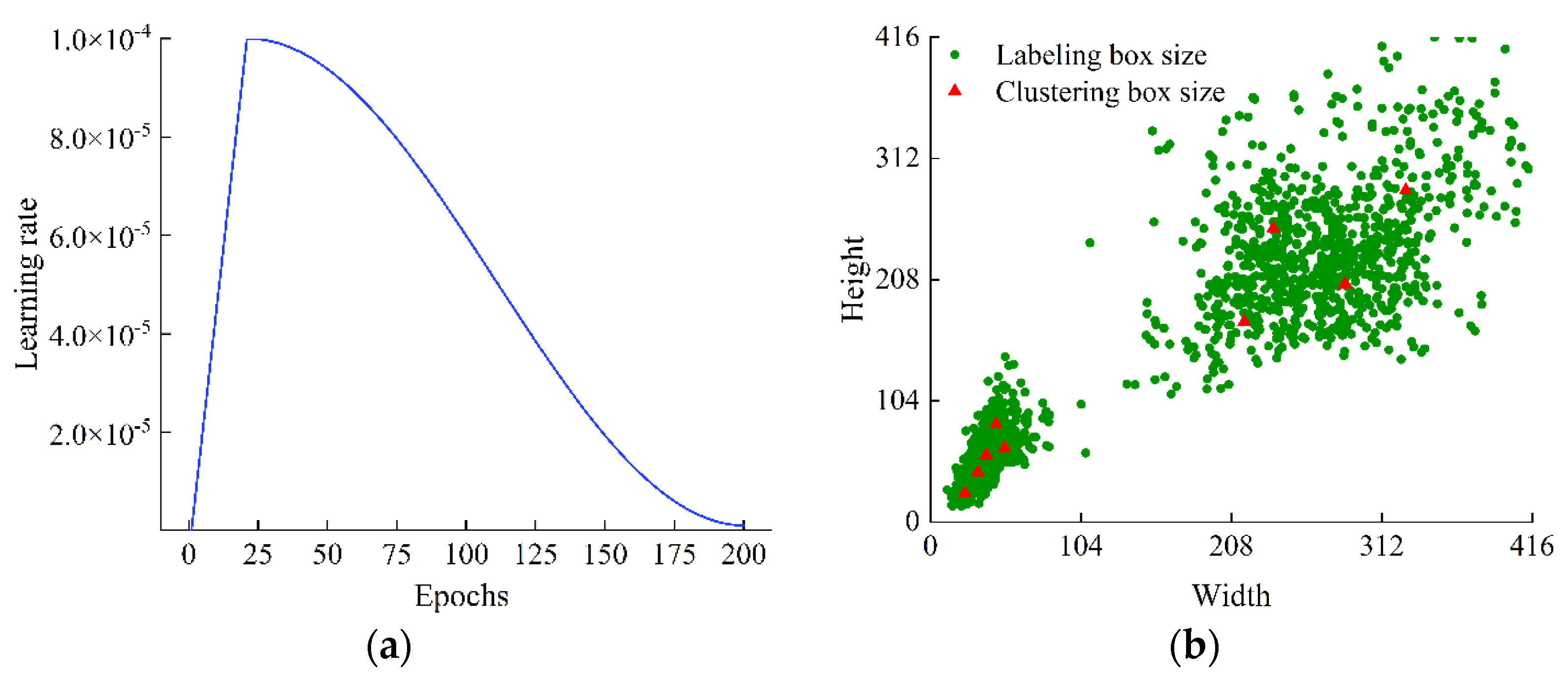
2.1.1. Data Acquisition and Annotation

This paper uses ginger seed samples collected from a ginger plantation in Anqiu, Shandong, China (36.47847° N, 119.2189° E) on 25 April 2021. The ginger seeds are of the ‘Baby Ginger’ variety and were germinated for 15 days. Ginger seed images were captured to accelerate the training and debugging of the ginger seed recognition model, by using the device shown in Figure 1, which includes a CMOS industrial camera, fill light, camera stand, computer, etc. The camera model was a MV-EM1400C manufactured by Micro-vision, with a resolution of 3288 × 3288 pixels; the fixed-focus lens was M1620-MPW2, the shooting distance was 30 cm, and a total of 500 images in “JPG” file format were stored. In addition, high luminance, regular luminance, and low luminance images were acquired separately to test the model recognition ability, for a total of 100 images. Meanwhile, 500 ginger seed images from a previous study by Hou et al. [27] were used to enrich the ginger dataset, with an image size of 5472 × 3672 pixels.

As shown in Figure 1, LabelImg (https://github.com/tzutalin/labelImg, accessed on 9 August 2021) was used to label the ginger shoots and ginger separately in “xml” file format, to determine the orientation of the ginger shoots; and it is worth noting that the labeled boxes are tightly aligned with the edges of the ginger and ginger shoots. In addition, the annotation information of each image was stored in a “txt” file, including image path, annotation box coordinates (image coordinates of the upper left and lower right corners), and object category. After image annotation, 1000 images were randomly divided into training and validation sets in the ratio of 80% and 20%, and the remaining 100 images were used for the model testing. Among them, the validation set was for adjusting the hyperparameters and monitoring the model for overfitting, and the test set was used for model evaluation, with no duplication between the above two, to ensure the accuracy of the model evaluation results. Finally, the ginger images, annotation files, and category labels were stored in PASCAL VOC format for training the ginger seed recognition network.

2.1.2. Data Enhancement

This paper used online data enhancement for expanding the original ginger seed images, to improve the model generalization ability and compensate for the insufficient number of samples. This means that before each batch training, the data-enhanced images were scaled to 416 × 416 pixels, and then four images were randomly cropped and stitched into one image using the Mosaic algorithm, thus, serving as training data. Mosaic greatly enriches the image background and also reduces the demand for GPU memory. The data enhancement methods are specified as follows: (1) Horizontal flip, mirror flip, and affine transformation were performed on images, with a 0.5 probability of reducing the effect of different ginger positions on the recognition results. (2) Image brightness was increased by 1.2 times or decreased by 0.8 times, with a 0.5 probability of reducing the effect of different illumination levels on the field on recognition results. (3) Image contrast was increased by 1.2 times or reduced by 0.8 times, with a 0.5 probability of better expressing the grayscale, sharpness, and texture details of the ginger images.

2.2. Overall Technical Route

To achieve accurate real-time detection of ginger and ginger seeds, the technical solutions proposed in this study are as follows:

• Construction and training of a YOLOv4-LITE network. This study used the MobileNetv2 network to replace the original CSPDarknet53, to solve the model redundancy caused by the more complex backbone network.
• The introduction of an attention mechanism and Do-Conv convolution. This study introduced an attention mechanism and Do-Conv into YOLOv4-LITE, to improve the recognition of smaller ginger shoots.
• Model performance analysis and experimental validation. The performance of the improved model was tested, and the improvements proposed in this study were verified and analyzed sequentially.

2.3. Method of Discriminating Ginger Shoot Orientation

2.3.1. YOLOv4 Model

As an end-to-end one-stage object detection algorithm based on regression theory, a YOLO network can directly predict the bounding box and class of an object. The YOLOv4 network is based on the original YOLO and is optimized for data processing, backbone network, activation function, loss function, and other aspects to improve the detection performance and inference speed of the model. Its training process is shown in Figure 2, which includes the following five parts:

• Based on Darknet53, CSPDarknet53 borrows the cross-stage partial (CSP) from CSPNet and adds a CSP on each of the five residual blocks, which enhances the learning ability of CNN and can maintain a high performance while lowering the weight of the network. CBL (convolution, batch normalization, and Leak-ReLU) is the most common module in YOLOv4 and includes convolutional (Conv) layers, batch normalization layers, and activation layer constructs.
• This paper adds a spatial pyramid pooling (SPP) structure after CSPDarknet53, which effectively increases the perceptual field of the backbone network. It uses the maximum pooling operations with convolution kernels of 1 × 1, 5 × 5, 9 × 9, and 13 × 13, respectively, to obtain four feature maps in different scales, and then fuses them in a concatenated manner.
• In CNN networks, shallow features contain richer target location information, such as contours and textures, and less semantic information. However, the deeper features contain richer semantic information, and the object location information is coarse. Therefore, our network adopts a feature pyramid network (FPN) structure, which passes the deep semantic information through up-sampling, thus fusing the shallow layers’ semantic information and location information.
• Borrowing from the bottom-up path augmentation method in PANet [49], two-path aggregation network (PAN) structures are added after FPN, which transmits the underlying location information by down-sampling, thus fusing location information with the semantic information of higher levels.
• YOLOv4 loss function includes bounding regression loss (L_coord), based on the complete intersection over union CIoU (L_CIoU), confidence loss (L_conf), and classification loss (L_cls). The loss function is formulated as follows:

$$\begin{array}{ll}\mathrm{Loss}& =L_{{}_{coord}}+L_{conf}+L_{c\mathrm{ls}}\\ & ={\lambda }_{\mathrm{coord}}{\displaystyle \sum _{i=0}^{s^2}{\displaystyle \sum _{j=0}^B{I}_{ij}^{\mathrm{obj}}}}\left(2-w_i*h_i\right)L_{CIoU}\\ & +{\displaystyle \sum _{i=0}^{s^2}{\displaystyle \sum _{j=0}^B\mathrm{BCE}(c_i,{\widehat{c}}_i)}}(I_{ij}^{\mathrm{obj}}+{\lambda }_{noobj}{I}_{ij}^{\mathrm{noobj}})\\ & +{\displaystyle \sum _{i=0}^{s^2}{I}_{ij}^{\mathrm{obj}}{\displaystyle \sum _{j=0}^B\mathrm{BCE}(p_i,}}{\widehat{p}}_i)\end{array}$$

(1)

where λ_coord and λ_noobj are penalty coefficients; s² is the number of grids in the feature map; B is the number of anchor boxes per grid; i is the i-th grid and j is the j-th anchor box; $(w_i, h_i)$ and $({\widehat{w}}_i, {\widehat{h}}_i)$ are the coordinates of the ground true and the prediction, respectively; BCE(·) represents the binary cross-entropy loss; $I_{ij}^{\mathrm{obj}}$ and $I_{ij}^{\mathrm{noobj}}$ represent whether there is an object in the j-th anchor box of the i-th grid, if so, then $I_{ij}^{\mathrm{obj}}=1$ and $I_{ij}^{\mathrm{noobj}}=0$, otherwise, $I_{ij}^{\mathrm{obj}}=0$ and $I_{ij}^{\mathrm{noobj}}=1$; $c_i$ and ${\widehat{c}}_i$ are the confidence of ground truth and prediction, respectively; $p_i$ and ${\widehat{p}}_i$ are the probabilities of the output categories of ground truth and prediction, respectively.

2.3.2. YOLOv4-LITE Network Design

Based on the features extracted by the backbone network, the YOLO network predicts object bounding boxes and categories. Moreover, YOLOv4 uses CSPDarknet53, after removing the final pooling layer, fully connected (FC) layer, and softmax layer, as the backbone of the feature extraction network. However, with YOLOv4 it is difficult to achieve a high inference speed in embedded devices, due to its network layer count of 104; requiring a lightweight network to replace the original complex backbone network. Therefore, this paper designed a YOLOv4-LITE network, based on the YOLOv4. In addition, MobileNetv1 is a lightweight network proposed by Google, and it uses depth-wise separable convolution instead of traditional convolution. Hence, this paper used MobileNetv2 as the backbone network of YOLOv4-LITE, which reduces the model size, while maintaining its performance. The network parameters of YOLOv4-LITE are shown in

Table 1. YOLOv4-LITE network parameters.

YOLOv4	No.	Type	Output Size	Stride	Numbers
MobileNetv2	-	Input	416 × 416 × 3	-	-
	0	CBL	208 × 208 × 32	2	1
	1–4	IRB2	208 × 208 × 16	2	1
	5–11	IRB1	104 × 104 × 24	1	2
	12–22	IRB2	52 × 52 × 32	2	3
	23-37	IRB2	52 × 52 × 64	2	4
	38-49	IRB1	26 × 26 × 96	1	3
	50–60	IRB2	13 × 13 × 160	2	3
	61–64	IRB2	13 × 13 × 320	2	1
	65	Conv 1 × 1	13 × 13 × 1280	1	1
SPP	66–68	CBL(F4)	13 × 13 × 640	1	3
	69–73	Max-pooling	13 × 13× 640	1	3
FPN + PANet	74–76	CBL	13 × 13 × 640	1	3
	77	CBL	13 × 13 × 48	1	1
	78	Up-sample	26 × 26 × 48	-	1
	79–80	Route + CBL	26 × 26 × 48	1	1
	81	Concatenate	26 × 26 × 96	-	1
	82–86	CBL(F3)	26 × 26 × 48	1	5
	87	CBL	26 × 26 × 16	1	1
	88	Up-sample	52 × 52 × 16	-	1
	89–90	Route + CBL	52 × 52 × 16	1	1
	91	Concatenate(F2)	52×52 × 32	-	1
	92–96	CBL(P2)	52 × 52 × 16	1	5
Head	97	CBL	52 × 52 × 32	1	1
	98	Conv 1 × 1	52 × 52 × 21	1	1
	99	Detection	-	-	1
FPN + PANet	100–101	Route + CBL	26 × 26 × 48	2	1
	102	Concatenate	26 × 26 × 96	-	1
	103–107	CBL(P3)	26 × 26 × 48	1	5
Head	108	CBL	26 × 26 × 96	1	1
	109	Conv 1 × 1	26 × 26 × 21	1	1
	110	Detection	-	-	1
FPN + PANet	111–112	Route + CBL	13 × 13 × 640	2	1
	113	Concatenate	13 × 13 × 1280	-	1
	114–118	CBL(P4)	13 × 13 × 640	1	5
Head	119	CBL	13 × 13 × 1280	1	1
	120	Conv	13 × 13 × 21	1	1
	121	Detection	-	-	1

.

As can be seen from Table 1, MobileNetv2 mainly consists of two forms of inverse residual block (IRB) that use depth-wise (DW) convolution and point-wise (PW) convolution to extract the image depth features, thus, greatly reducing the time complexity and space complexity of the convolution operations. Figure 3 is a schematic diagram of the improved backbone network. As shown in Figure 3, when stride = 1 in DW convolution, the block is the inverse residual block 1 (IRB₁); when stride = 2 in DW convolution, the block is the inverse residual block 2 (IRB₂). Since the convolutional layer in IRB₂ also has a down-sampling function, shortcut is not used to keep the output dimension consistent. The above two kinds of IRBs are composed of PW₁ convolution, DW convolution, and PW₂ convolution. Among them, PW₁ convolution consists of 1 × 1 convolution, BN, and ReLU6, and it maps the feature dimension, from low-dimensional space to high-dimensional space, which is beneficial for feature extraction; DW convolution is composed of 3 × 3 convolution, BN, and ReLU6, and realizes feature extraction; the PW₂ convolution is composed of 1 × 1 convolution and BN to map the high-dimensional space to the low-dimensional space. As the ReLU6 activation function would destroy the features learned by the CNN in the low-dimensional space, the PW₂ convolution is not followed by an activation function.

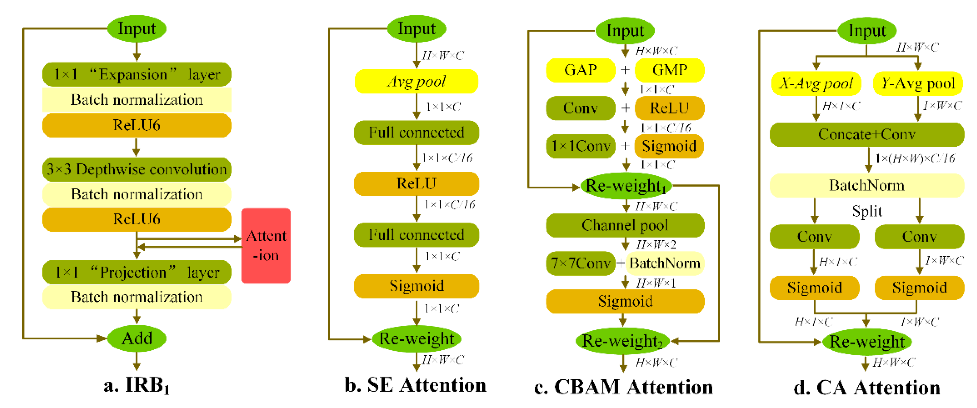
2.3.3. Coordinate Attention Module

In this paper, an attention [50] mechanism is introduced to improve the model accuracy, by selecting the most critical information for the current recognition task from a large amount of feature information. This is essentially similar to human selective vision, in that it quickly scans the global image to obtain the information that needs to be focused on, while suppressing information that is not helpful for the current task. Therefore, the attention mechanism is applied after DW convolution in the IRB of MobileNetv2. Figure 4 shows the schematic diagram of different attention mechanisms, with an input feature map of size: Height (H) × Width (W) × Channel (C).

Figure 4b shows a schematic structure of SE attention. As the convolution operation only integrates the information of the spatial dimension and channel dimension within a local perceptual field, it does not obtain enough information between global channels. Therefore, first, global average pooling (GAP) is used to compress feature 1 (H × W × C), which has global spatial information, into feature 2 (1 × 1 × C), which has a global receptive field. Second, two FC layers are used to reduce the complexity and improve the generalization ability of the network; where the first FC is used to reduce the dimensionality of the feature map, and the second FC is used to recover the feature dimensionality. Third, feature 3 (1 × 1 × C) is obtained after the sigmoid activation function, which characterizes the importance of each channel. Finally, the channels of feature 3 are multiplied one by one with feature map 1 to obtain the final output re-weight (H × W × C), which is equivalent to adding a weight to each channel of feature 1, thus giving greater weight to information helpful for the task at hand. In conclusion, SE attention improves the sensitivity of the network to channel features and contributes a performance improvement by lowering the computation needed, but it ignores the importance of the location feature information.

Figure 4c shows a schematic structure of CBAM attention, including the channel attention module (CAM) and spatial attention module (SAM). On the one hand, CAM is similar to SE attention, in that it first compresses the input feature 1 (H × W × C) into feature 2 (1 × 1 × C) using GAP and global max pooling (GMP), which adds a layer of GMP with respect to SE attention; thus, increasing the feature dimension once again. Second, feature 2 is first reduced in the channel dimension to C/16 using a convolution layer, and then its dimension is raised using 1 × 1 convolution to obtain feature 3 (1 × 1 × C). Third, feature 4 (H × W × 1) is gained after the sigmoid activation function, which characterizes the importance of the channel feature information. Finally, the Re-weight₁ (H × W × C) is obtained by multiplying feature 4 with feature 1. On the other hand, in the SAM, first, Re-weight₁ is compressed into feature 5 (H × W × 1) and features 6 (H × W × 1) along the channel direction, using GAP and GMP, respectively, and then they are concatenated based on the channel direction to obtain feature 7 (H × W × 2). Second, the channel dimension of feature 7 is reduced to 1 using 7 × 7 convolution, resulting in feature 8 (H × W × 1). Third, feature 9 (H × W × 1) is gained after sigmoid activation, and this characterizes the importance of the location feature information. Finally, the final output Re-weight₂ (H × W × C) is obtained by multiplying feature 9 with Re-weight₁, which is equivalent to adding a weight to the location features of Re-weight₁, so that the location helpful information for the current task has greater weight.

The above two attention mechanisms are widely used in lightweight networks and have achieved good results. However, SE attention only considers the channel feature information and ignores the location information, and CBAM attention only introduces local location information through global pooling. Therefore, this paper presents a coordination attention mechanism, in which location information is embedded into channel attention to avoid adding a large amount of additional computational overheads, while ensuring better attention results for MobileNetv2. Figure 4d shows a schematic structure of CA attention, consisting of coordinate information embedding and coordinate attention generation. Each channel is first encoded along two spatial directions, vertical and horizontal, using GAP with pooling kernel sizes (H, 1) and (1, W), respectively, to avoid a possible loss of valuable location information by global pooling in channel attention. The above enables the input feature map 1 (H × W × C) to be compressed into a pair of direction-aware features, including feature 2 (H × 1 × C) and feature 3 (1 × W × C), and they have global receptive field and precise location information. Second, feature 4 (1 × (H + W) × (C/16)) is obtained after concatenating feature 2 with 3 and reducing the feature dimension using 1×1 convolution. Then, feature 4 is decomposed into feature 5, 6 along the spatial dimension, and their feature dimensions are elevated using 1 × 1 convolution, and the above operation greatly reduces the model complexity and computational overhead. Finally, features 5 and 6 are multiplied with feature 1 after sigmoid activation to obtain the final output Re-weight₂ (H × W × C).

2.3.4. Do-Conv Convolution

In general, the network depth is usually increased by combining linear convolutional layers and nonlinear network layers to increase the network expressiveness, since successive linear layers increase the overfitting phenomenon of the network and can be replaced by a linear layer. This paper replaces part of the traditional convolution in FPN + PANet with Do-Conv convolution, speeding up the network training and promoting the model convergence.

The operation of Do-Conv is shown in Figure 5, where * denotes conventional convolution and ∘ denotes depth-wise convolution. In model training, the depth-wise convolution of weight ${\mathbb{D}}^T\in R^{(M\times N)\times C_{in }}$ and weight $\mathbb{W}\in R^{D_{mu}\times C_{in}\times C_{out}}$ are first computed to obtain the new weight ${\mathbb{W}}^{\prime }\in R^{M\times N\times C_{in}\times C_{out}}$, and then the conventional convolution of weights $\mathbb{W}\prime$ and input features $\mathbb{P}$ is calculated to get the final output $\mathbb{O}$, and it should be noted that $D_{mul}\ge M\times N$. On the basis of traditional convolution, Do-Conv adds an additional depth-wise convolution, to form an over-parameterized convolution layer, which increases the number of parameters compared to conventional convolution. Although the number of parameters increases, the multi-layer linear operations used in over-parameterized convolution can be combined into a single-layer convolution operation during model inference, because both conventional convolution and depth-wise convolution are linear operations, thus speeding up the inference.

2.3.5. Focal Loss Function

In the YOLOv4-LITE network training, it is necessary to first set a suitable intersection over union (IoU) threshold. When the IoU between the anchor box and all targets ground truth is less than the IoU threshold, this anchor box is regarded as a negative sample; and when the target centroid falls in a grid, the anchor box in the grid that has the maximum IoU with the target is a positive sample. In one-stage object detection, the loss function is dominated by many negative samples due to the imbalance between positive and negative samples during training, so the network cannot measure the prediction results. Therefore, this paper introduces a focal loss function to solve the problems of unbalanced positive and negative samples, and unbalanced simple samples and difficult samples. The focal loss function is calculated as follows:

$$FL(p_t,y)=\{\begin{array}{l}-\alpha {\left(1-p_t\right)}^{\gamma }{\log }_a{p}_t,y=1\\ -\left(1-\alpha \right)p_t{}^{\gamma }{\log }_a\left(1-p_t\right),y=0\end{array}$$

(2)

where y is the category label and p_t (p_t ∈ [0, 1]) is the probability that the t-th sample is y. Considering the imbalance of positive and negative samples in the ginger image, most of the area is the background, and the number of positive samples (ginger and ginger shoots) is much lower than the negative samples (background). Thus, the paper adds a weighting factor α (α ∈ [0.5, 1)) to the cross-entropy loss function so that a smaller number of positive samples take up more weight, and thus the model can learn more helpful information. On the other hand, considering the imbalance between simple and difficult samples, ginger samples are more facile to identify than ginger shoot samples. Focal loss combines the idea of OHNM, by adding a weighting factor (1 − p_t)^γ to the loss function, and γ can be used to reduce the loss of simple samples by adjusting the variation range of weighting factor (1 − p_t)^γ, and its value range is generally [0, 5]. For instance, when y_t = 1, the p_t of the simple sample is close to 1, so (1 − p_t)^γ is close to 0. In contrast, (1 − p_t)^γ of the difficult sample is close to 1. The above description implies that the addition of (1 − p_t)^γ makes the difficult samples have a more significant impact on the loss function. If γ is too small, it will not increase the loss of difficult samples. On the contrary, if γ is too large, it is not conducive to model training. In the end, γ = 2 and α = 0.75.

2.3.6. Identification Method of Ginger Shoot Orientation

First, to discriminate the orientation of ginger shoots, the location of the ginger shoots and ginger is predicted using the ginger identification network. Second, this paper uses the area of the ginger shoot prediction box as the criterion to select ginger shoot and only selects the largest one to discriminate the orientation of ginger shoot. As shown in Figure 6, a right-angle coordinate system is established with the center point O of the ginger prediction frame as the origin, the center point of the ginger prediction frame is A (dx, dy), and the orientation angle of the ginger shoot is θ, where “+” indicates counterclockwise rotation and “−” indicates clockwise rotation.

$$\theta \prime =\arctan (\frac{\left|dy\right|}{\left|dx\right|})$$

(3)

$$\theta =\{\begin{array}{l}+\theta \prime , \mathrm{d}x>0 \mathrm{d}y\ge 0\\ +\mathsf{\pi }/2, \mathrm{d}x=0 \mathrm{d}y>0\\ +(\mathsf{\pi }-\theta \prime ), \mathrm{d}x<0 \mathrm{d}y>0\\ -(\mathsf{\pi }-\theta \prime ), \mathrm{d}x<0 \mathrm{d}y\le 0\\ -\mathsf{\pi }/2, \mathrm{d}x=0 \mathrm{d}y<0\\ -\theta \prime , \mathrm{d}x>0 \mathrm{d}y<0\end{array}$$

(4)

2.4. Method of Discriminating Ginger Shoot Orientation

The paper uses precision (P) and recall (R) as evaluation criteria to assess the model performance. In addition, the F1 score can be used to equalize the precision and recall. They are defined as shown in Equations (5)–(7).

$$P=\frac{TP}{TP+FP}\times 100\%$$

(5)

$$R=\frac{TP}{TP+FN}\times 100\%$$

(6)

$$\mathrm{F}1 \mathrm{score}=\frac{2PR}{P+R}\times 100\%$$

(7)

where true positive (TP) means that the prediction result and ground truth are both positive samples; false positive (FP) indicates that the prediction result is positive and ground truth is negative; and false negative (FN) means the prediction result is negative and ground truth is positive.

However, depending on different task requirements, precision and recall can be adjusted to various values during model testing by adjusting different confidence thresholds, and average precision (AP), as the average of precision under different recalls can be used to measure the inherent model properties. In this study, since there are two categories, the ginger shoot and ginger seeds, mean average precision (mAP) was adopted to measure the model performance. The equations of AP and mAP are as follows:

$$AP={\displaystyle {\int }_0^{1}P\left(R\right)dR}\times 100\%$$

(8)

$$mAP=\frac{1}{2}{\displaystyle \sum _{m=0}^1{\displaystyle {\int }_0^1{P}_m(R_m)d{R}_m}\times 100\%}$$

(9)

where m is the number of categories and R is the integral variable used to calculate the region’s area under the P-R curve. AP₅₀ is the AP value when the IoU threshold is 0.5; therefore, mAP₅₀ is the average of AP₅₀ for all categories. Similarly, mAP₇₅ is the average of AP₇₅ of all categories, mAP_50:95 is the average of AP_50:95, and AP_50:95 is the average of ten values of AP₅₀, AP₅₅, AP₆₀, …, AP₉₅.

In addition, the model performance was measured using model size, Params, and giga Flops (GFlops) [50,51], where Params is the total number of parameters required to train the network, and GFlops is the amount of computation in the network. The lower the GFlops, the less computation and execution time needed for the model.

3. Results and Discussion

The experimental environment of the YOLOv4-LITE network during model training is shown in

Table 2. Experimental environment.

Configuration	Parameter
CPU	Intel core I9-9900K
GPU	Nvidia GTX 2080Ti GPU
Operating system	Ubuntu 18.04
Accelerated environment	CUDA 10.0 CUDNN 7.0
Development environment	PyCharm professional edition
Library	Python 3.6, Pytorch1.5.1, Opencv4.2.0

. In addition, the model optimizer was SGD (stochastic gradient descent), the momentum was 0.95, the weight attenuation coefficient was 5 × 10⁻³, the batch size was 16, the trained epochs were 200, and the model weight was reserved once for every 10 epochs. At the beginning of the network training, the learning rate was increased linearly from 0 to 1 × 10⁻⁴ in the first 20 epochs, to make the network converge to a better initial state quickly, and it was then reduced to 1 × 10⁻⁶ by using the cosine annealing decay method; the formula and diagram of the learning rate are shown below.

$$lr=\{\begin{array}{l}\frac{l{r}_{max}}{T_{warm}}t t\le T_{warm}\\ l{r}_{min}+\frac{1}{2}\left(l{r}_{max}-l{r}_{\min }\right)\left(1+\cos (\frac{\mathrm{t}-T_{warm}}{T_{total}})\right) t>T_{warm}\end{array}$$

(10)

where t and T_warm are the current epochs and warmup epochs, respectively; lr_min and lr_max represent the minimum and maximum values of the learning rate, respectively; T_cur and T_total represent the current and total epochs, respectively.

As shown in Figure 7b, the dimensions of the labeled boxes were clustered using the K-means algorithm before network training. K-means uses an IoU-based metric with the objective function of minimizing the distance between the labeled boxes and the clustered boxes, and resulted in nine clustered boxes, (24, 24), (33, 42), (39, 57), (51, 64), (46, 84), (217, 172), (287, 204), (237, 252), and (329, 285), which were then used to initialize the anchor boxes in the ginger recognition network. When network training, a multi-scale training method is used to improve the model generalization, which means randomly training the model with images of different sizes every 10 batches, while ensuring that the image edge length is a multiple of 32. Moreover, this paper also used mixed-precision training, based on single-precision and half-precision, to speed up the network training and reduce the GPU memory usage.

3.1. Result Analysis

As is well-known, the loss function evaluates a model by measuring the error between the predicted and the true values. Figure 8a shows the loss value change curve of YOLOv4-LITE with a total training time of 3.5 h. As seen in Figure 8a, the loss value dropped rapidly from 1441.33 to 3.71 in the first 40 epochs and then slowly oscillated down and stabilized as the epochs increased. Eventually, the loss value stabilized at around 1.80, and the model converged at the same time point. Figure 8b shows the P-R curves for an IoU threshold of 0.5. Both the P-R curves for ginger shoots and ginger enclosed almost the entire parameter space, which indicated that the model had achieved a sufficient average precision. It can also be clearly seen from Figure 8b that YOLOv4-LITE performed better in ginger recognition than the ginger shoots of smaller targets.

The test results of the validation set were analyzed, and the confidence threshold (conf-thresh) was taken as 0.5, and the IoU threshold was taken as 0.5. The test results are shown in

Table 3. Validation set test results after network improvement (conf-thresh = 0.5, IoU = 0.5).

Model	TP	FP	FN	P/%	R/%	F1-Score/%
YOLOv4	414	23	21	94.74	95.17	94.95
YOLOv4-LITE	419	21	16	95.23	96.32	95.77

, and the number of the ground truth in the test set was 435. The improved model had improvements in terms of precision, recall, and F1-score. Specifically, the precision increased by 0.49%, recall increased by 1.15%, and F1-score increased by 0.82%. The analysis of TP, FP, and FN in the test results revealed that the improved model performance mainly depended on the increase of TP and the decrease of FP and FN.

As shown in Figure 9a,b, this paper compared the original and manually labeled ginger seed images to better evaluate the recognition effect of the YOLOv4-LITE network. The final recognition results are as shown in Figure 9c, where the sizes of the test images are all 416 × 416 pixels, and the green and white rectangular boxes represent the predicted boxes for the ginger and ginger shoots, respectively. As can be seen in Figure 9, the ginger seed images were well recognized. The image above had only one ginger shoot, and the coordinates of the center points of the prediction boxes for ginger and shoot were (204, 207) and (220, 317), respectively. After the calculation of Equations (3) and (4), δ = −81.7°, the ginger seed was rotated clockwise by 81.7° to ensure consistent ginger shoot orientation. The below image had two ginger shoots, as shown by the red arrows, only the ginger shoot with the larger prediction box was chosen. The coordinates of the center points of the prediction boxes for ginger and shoot are (191, 192) and (270, 238), respectively. After the calculation of Equations (3) and (4), δ = −30.2°, the ginger seed should be rotated clockwise by 30.2°.

Due to the very irregular shape of the ginger seeds and the fragility of the ginger shoots, we designed a ginger seed transport channel. After placing the ginger seeds on the channel, detection of the seeds and the orientation of the ginger shoots was achieved using an image acquisition device and a mobile terminal device. Next, an end-effector with vacuum suction cups was used to pick up the center of the ginger prediction box and adjust the orientation of the ginger shoot in real-time to ensure that the ginger shoots were facing the same direction.

3.2. Discussion of the Improved Algorithm

This paper conducted the following three comparison experiments [52] to demonstrate the contribution of the proposed improved refinements to the YOLOv4 network: comparison experiments after replacing the feature extraction network, experiments with different attention mechanisms, and comparison experiments after adding Do-Conv convolution.

3.2.1. Performance Comparison of Feature Map Extraction Network

The test results of the network are as shown in Figure 10, after replacing the original backbone network of YOLOv4 with the MobileNetv2 network. This strategy achieved good results, as mAP₅₀ was reduced by only 0.37%. Moreover, compared to the original CSPDarknet53, the network computation was greatly reduced after using MobieNetv2 as the backbone network. As shown in

Table 4. Experimental results under different feature extraction networks.

Backbone Network	AP50/% (Shoot)	AP50/% (Ginger)	Size/MB	Params/M	GFlops
CSPDarknet53	98.22	99.99	264.6	63.94	29.883
MobileNetv2	97.45	99.99	115	47.99	8.741

, the model size, Params, and GFlops before and after the improvement of the backbone network were compared, and, notably, when calculating Params and GFlops, the network input images were of the same size, and 416 × 416 pixels was chosen for this paper. As can be seen from Table 4, YOLOv4-LITE using MobieNetv2 as the backbone network was much smaller than the original network, in terms of model size, Params, and GFlops; reducing these to 149.6 MB, 15.95 M, and 21.14, respectively, which indicated that the improved network had a lower computational time and spatial complexity.

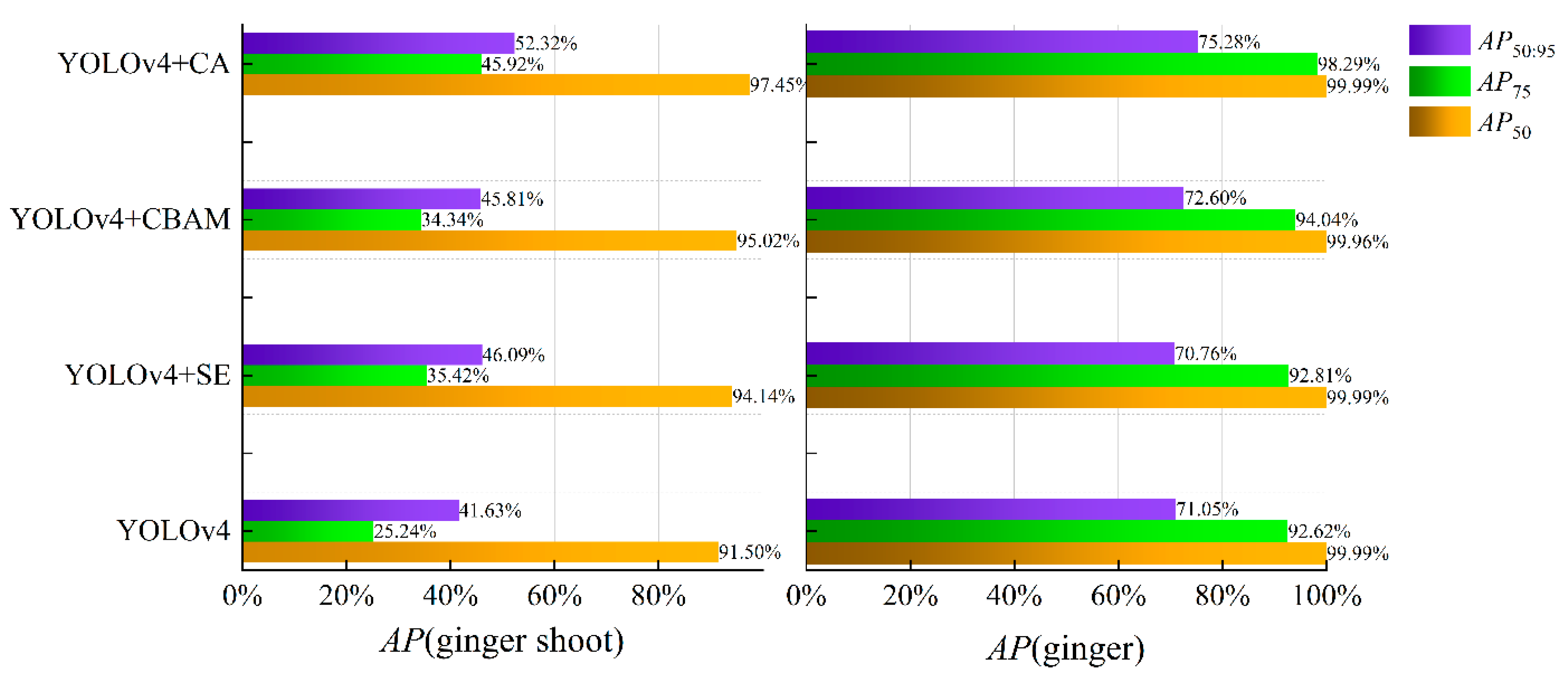
3.2.2. Different Attention Mechanisms Comparative Experiment

In this paper, SE, CBAM, and CA attentions were inserted in the IRB module of MobileNetv2 to verify the effect of CA attention by comparing their test results. The test results shown in Figure 11 indicated that after using three kinds of attention modules, the AP₅₀ of ginger shoots increased by 2.64%, 3.52%, and 5.95%, respectively, while the AP₅₀ of ginger remained basically unchanged. It is worth mentioning that the AP of ginger shoots improved most significantly after using CA attention, with AP₅₀ increasing from 91.5% to 97.45% and AP_50:95 rising from 41.63% to 52.32%, indicating that the addition of CA attention to YOLOv4-LITE effectively improved the detection accuracy of ginger shoots.

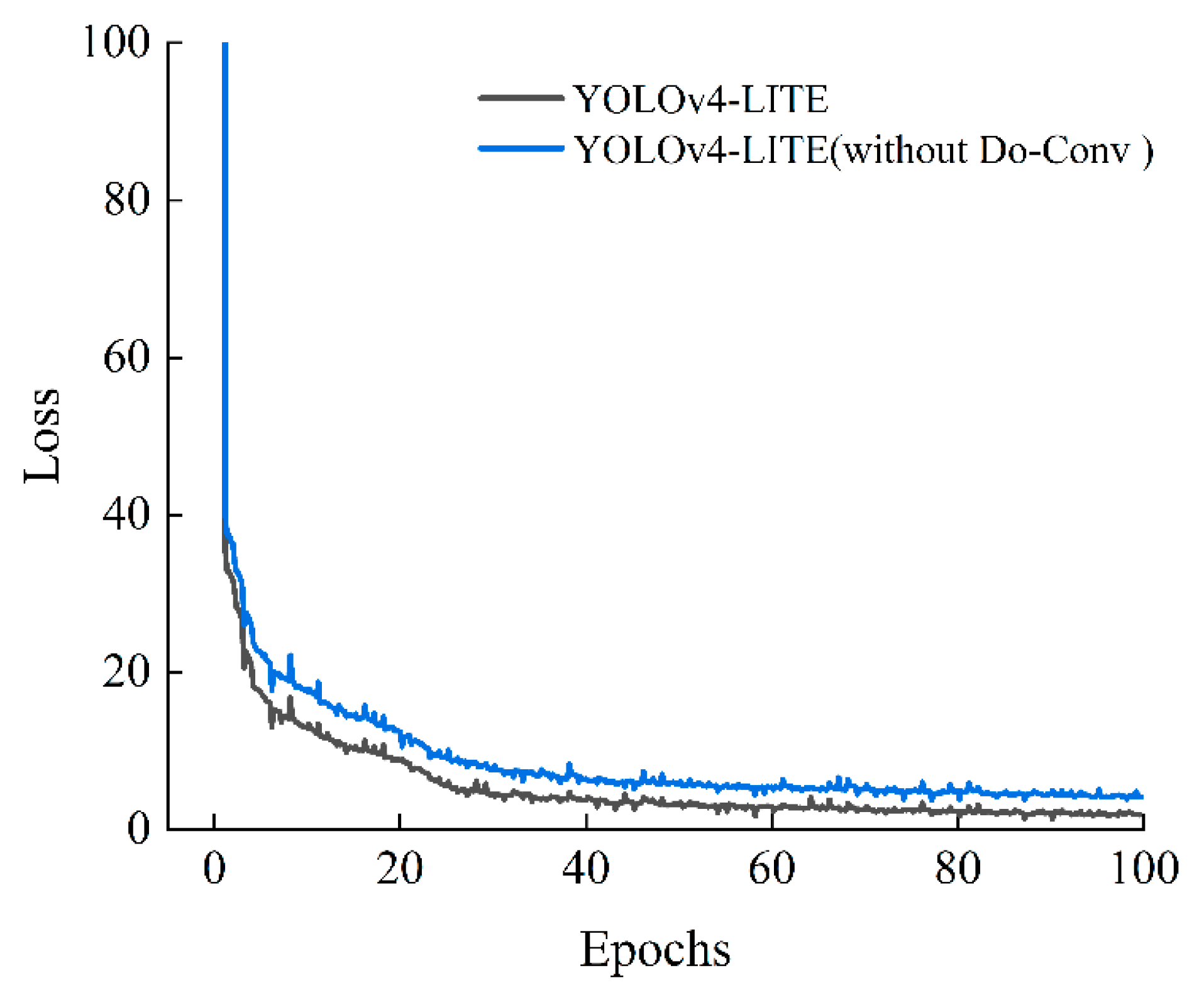
3.2.3. Analysis of Do-Conv Convolution

This paper conducted a comparison experiment with Do-Conv instead of the conventional convolution in the FPN + PANet structure, to study the effect of Do-Conv convolution on the ginger seed recognition network. The loss curves of the YOLOv4-LITE network are shown in Figure 12, which indicate that the network had a faster convergence rate after using Do-Conv convolution in the training process. Moreover, the network test results after using Do-Conv are shown in

Table 5. Testing set experiment results using Do-Conv.

Model	AP50/% (Ginger Shoot)	AP50/% (Shoot)	mAP/%	Params/M	GFlops
YOLOv4-LITE	97.45	99.99	98.72	47.99	8.741
YOLOv4-LITE (without Do-Conv)	95.27	99.99	97.63	47.99	8.741

, which show that the AP₅₀ of ginger shoots improved by 2.18%. Furthermore, although the Do-Conv convolution layer added an extra depth-wise convolution to the conventional convolution, it did not increase the Params and GFlops. The reason for this was as follows: during the model training, $\mathbb{D}$ and $\mathbb{W}$ were folded into $\mathbb{W}\prime$($\mathbb{W}\prime ={\mathbb{D}}^T\circ \mathbb{W}$) with the same shape as the conventional convolution kernel that they replaced, so the Params and GFlops of the model did not change in the inference.

3.3. Performance Comparison of the Overall Algorithm

Figure 13 shows the mAP of the various improved algorithms. Compared with YOLOv3 and YOLOv3-tiny [53], YOLOv4 had a better target detection performance, with a mAP₅₀ of 99.1%, which was 1% and 1.8% higher than the others, respectively. When replacing the backbone network with MobileNetv3 [54], Ghost-Net [55], and MobileNetv2, without using other improved strategies, the network detection performance dropped dramatically, with a mAP₅₀ of only 92.75%, 93.13%, and 93.54%. After using CA attention or Do-Conv based on MobileNetv2, the mAP₅₀ reached 97.63% and 97.25%, respectively; while, after using CA attention and Do-Conv at the same time, mAP₅₀ reached 98.73%. In summary, this study effectively enhanced the network performance through the series of improvements mentioned above.

For the recognition of ginger seed images, we tried to use the traditional color difference segmentation method to segment ginger shoots and recorded the color components of ginger seed images using RGB (red green blue) and HSV (hue saturation value). It was found that the H component is less influenced by the illumination and can achieve the segmentation of ginger shoots. However, the ginger seeds were treated with drugs resulting in unstable color characteristics of the ginger shoots, thus making the error rate of identification high; therefore, the color difference segmentation method is not very reliable for the segmentation of ginger shoots.

Unlike the traditional color difference segmentation method, Hou et al. proposed a fast recognition method for ginger shoots based on YOLOv3. The method avoided the manual design of feature extractors and had good robustness, and the AP of ginger shoots reached 98.2%. However, it only identified ginger shoots and did not identify ginger, resulting in a complex calculation process for ginger shoot orientation. In addition, its backbone network was complex and contained a large number of redundant parameters, making it difficult to deploy on ginger seeders and also restricting the development of automated ginger seeders to some extent.

Based on the constructed ginger seed dataset, the backbone network of YOLOv4 was replaced by MobileNetv2, which greatly reduced the network parameters and computational effort. Meanwhile, CA attention and Do-Conv convolution were added to the backbone network to improve the detection of ginger shoots and the convergence speed of the model. The experimental results showed that mAP₅₀ reached 98.72% and mAP₇₅ reached 82.46%.

4. Conclusions

To achieve ginger seed detection and ginger shoot orientation discrimination, this paper introduced an improved YOLOv4-LITE network to detect ginger shoots and ginger in ginger seed images and then discriminated ginger shoot orientation by calculating the position of the largest ginger shoot relative to the ginger. First, this paper replaced the original CSPDarknet53 backbone network with MobileNetv2, which significantly reduced the network parameters and computation; thus, facilitating migration of the network to a mobile terminal. Second, a coordinate attention mechanism was added into the backbone network to improve the detection of ginger shoots. Third, Do-Conv was adopted to replace some traditional convolutions, thus improving the model convergence speed. Finally, the paper also used focal loss to solve the imbalance between positive and negative samples and the imbalance between simple and difficult samples in the ginger dataset.

The experimental results showed that the mAP₅₀ of the proposed improved YOLOv4-LITE network reached 98.73%. Compared with the original YOLOv4, its Params and GFlops decreased by 15.95 M and 21.14, respectively, while the mAP₅₀ was only reduced by 0.37%. This indicates that using the improved backbone network and Do-Conv convolution is effective for improving the performance of the ginger seed recognition network.

References

1. Retana-Cordero, M.; Fisher, P.R.; Gómez, C. Modeling the Effect of Temperature on Ginger and Turmeric Rhizome Sprouting. Agronomy 2021, 11, 1931. [Google Scholar] [CrossRef]
2. Sang, S.; Snook, H.D.; Tareq, F.S.; Fasina, Y. Precision Research on Ginger: The Type of Ginger Matters. J. Agric. Food Chem. 2020, 68, 8517–8523. [Google Scholar] [CrossRef]
3. Liu, S.; Chen, M.; He, T.; Ren, C. Review of China’s ginger market in 2018 and market outlook in 2019. China Veget. 2019, 2, 1–4. [Google Scholar]
4. Zhang, K.; Jiang, H.; Liu, P.; Zhang, Y. Prediction of ginger planting area based on GM(1,N) model. J. Chin. Agric. Mech. 2020, 41, 139–143. [Google Scholar]
5. Tao, W. Technical specifications for the safe production of ginger. In Laiwu Ginger, 1st ed.; China Agricultural Science and Technology Press: Beijing, China, 2010; pp. 78–79. [Google Scholar]
6. Mahender, B.; Reddy, P.S.S.; Sivaram, G.T.; Balakrishna, M.; Prathap, B. Effect of seed rhizome size and plant spacing on growth, yield and quality of ginger (Zingiber officinale rosc.) under coconut cropping system. Plant Arch. 2015, 15, 769–774. [Google Scholar]
7. Liu, J. Biological properties of ginger. In Laiwu Ginger, 1st ed.; China Agricultural Science and Technology Press: Beijing, China, 2013; pp. 76–77. [Google Scholar]
8. Hordofa, T.S.; Tolossa, T.T. Cultivation and postharvest handling practices affecting yield and quality of major spices crops in Ethiopia: A review. Cogent Food Agric. 2020, 6. [Google Scholar] [CrossRef]
9. Ren, S.; Li, C. Analysis of the current situation and development of the ginger industry in China. China Veget. 2021, 8, 8–11. [Google Scholar]
10. Xiong, X.; Duan, L.; Liu, L.; Tu, H.; Yang, P.; Wu, D.; Chen, G.; Xiong, L.; Yang, W.; Liu, Q. Panicle-SEG: A robust image segmentation method for rice panicles in the field based on deep learning and superpixel optimization. Plant Methods 2017, 13, 1–15. [Google Scholar] [CrossRef] [Green Version]
11. Li, H.; Wang, G.; Dong, Z.; Wei, X.; Wu, M.; Song, H.; Amankwah, S.O.Y. Identifying Cotton Fields from Remote Sensing Images Using Multiple Deep Learning Networks. Agronomy 2021, 11, 174. [Google Scholar] [CrossRef]
12. Gahrouei, O.; McNairn, H.; Hosseini, M.; Homayouni, S. Estimation of Crop Biomass and Leaf Area Index from Multitemporal and Multispectral Imagery Using Machine Learning Approaches. Can. J. Remote Sens. 2020, 46, 84–99. [Google Scholar] [CrossRef]
13. Bahrami, H.; Homayouni, S.; Safari, A.; Mirzaei, S.; Mahdianpari, M.; Reisi-Gahrouei, O. Deep Learning-Based Estimation of Crop Biophysical Parameters Using Multi-Source and Multi-Temporal Remote Sensing Observations. Agronomy 2021, 11, 1363. [Google Scholar] [CrossRef]
14. Wang, C.; Xiao, Z. Lychee Surface Defect Detection Based on Deep Convolutional Neural Networks with GAN-Based Data Augmentation. Agronomy 2021, 11, 1500. [Google Scholar] [CrossRef]
15. Guo, Q.; Wang, C.; Xiao, D.; Huang, Q. An Enhanced Insect Pest Counter Based on Saliency Map and Improved Non-Maximum Suppression. Insects 2021, 12, 705. [Google Scholar] [CrossRef]
16. Parvathi, S.; Selvi, S.T. Detection of maturity stages of coconuts in complex background using Faster R-CNN model. Biosyst. Eng. 2021, 202, 119–132. [Google Scholar] [CrossRef]
17. Ren, S.; He, K.; Girshick, R.; Sun, J. Faster R-CNN: Towards real-time object detection with region proposal networks. IEEE Trans. Pattern Anal. Mach. Intell. 2017, 39, 1137–1149. [Google Scholar] [CrossRef] [PubMed] [Green Version]
18. Jiao, L.; Dong, S.; Zhang, S.; Xie, C.; Wang, H. AF-RCNN: An anchor-free convolutional neural network for multi-categories agricultural pest detection. Comput. Electron. Agric. 2020, 174, 105522. [Google Scholar] [CrossRef]
19. He, K.; Gkioxari, G.; Dollár, P.; Girshick, R. Mask R-CNN. In Proceedings of the 2017 IEEE International Conference on Computer Vision (ICCV), Venice, Italy, 22–29 October 2017. [Google Scholar]
20. Ammar, A.; Koubaa, A.; Benjdira, B. Deep-Learning-Based Automated Palm Tree Counting and Geolocation in Large Farms from Aerial Geotagged Images. Agronomy 2021, 11, 1458. [Google Scholar] [CrossRef]
21. Kuznetsova, A.; Maleva, T.; Soloviev, V. Using YOLOv3 Algorithm with Pre- and Post-Processing for Apple Detection in Fruit-Harvesting Robot. Agronomy 2020, 10, 1016. [Google Scholar] [CrossRef]
22. Redmon, J.; Divvala, S.; Girshick, R.; Farhadi, A. You only look once: Unified, real-time object detection. In Proceedings of the 2016 IEEE Conference on Computer Vision and Pattern Recognition (CVPR), Las Vegas, NV, USA, 27–30 June 2016. [Google Scholar]
23. Suo, R.; Gao, F.; Zhou, Z.; Fu, L.; Song, Z.; Dhupia, J.; Li, R.; Cui, Y. Improved multi-classes kiwifruit detection in orchard to avoid collisions during robotic picking. Comput. Electron. Agric. 2021, 182, 106052. [Google Scholar] [CrossRef]
24. Wu, D.; Lv, S.; Jiang, M.; Song, H. Using channel pruning-based YOLO v4 deep learning algorithm for the real-time and accurate detection of apple flowers in natural environments. Comput. Electron. Agric. 2020, 178, 105742. [Google Scholar] [CrossRef]
25. Liu, W.; Anguelov, D.; Erhan, D.; Szegedy, C.; Reed, E.S.; Fu, C.-Y.; Berg, A.C. SSD: Single shot multiBox detector. In Proceedings of the 14th European Conference on Computer Vision (ECCV), Amsterdam, The Netherlands, 11–14 October 2016. [Google Scholar]
26. Lin, T.; Goyal, P.; Girshick, R.; He, K.; Dollár, P. Focal Loss for Dense Object Detection. IEEE Trans. Pattern Anal. Mach. Intell. 2020, 42, 318–327. [Google Scholar] [CrossRef] [Green Version]
27. Koirala, A.; Walsh, K.B.; Wang, Z.; Anderson, N. Deep Learning for Mango (Mangifera indica) Panicle Stage Classification. Agronomy 2020, 10, 143. [Google Scholar] [CrossRef] [Green Version]
28. Hou, J.; Fang, L.; Wu, Y.; Li, Y.; Xi, R. Rapid recognition and orientation determination of ginger shoots with deep learning. Trans. Chin. Soc. Agric. Eng. 2021, 37, 213–222. [Google Scholar]
29. Cai, K.; Miao, X.; Wang, W.; Pang, H.; Liu, Y.; Song, J. A modified YOLOv3 model for fish detection based on MobileNetv1 as backbone. Aquac. Eng. 2020, 91, 102117. [Google Scholar] [CrossRef]
30. Yu, Y.; Zhang, K.; Liu, L.H.; Yang, L.; Zhang, D.X. Real-time visual localization of the picking points for a ridge-planting strawberry harvesting robot. IEEE Access 2020, 8, 116556–116568. [Google Scholar] [CrossRef]
31. Lui, S.; Lu, S.; Li, Z.; Hong, T.; Xue, Y.; Wu, B. Orange recognition method using improved YOLOv3-LITE lightweight neural network. Trans. Chin. Soc. Agric. Eng. 2019, 35, 205–214. [Google Scholar]
32. Ying, B.; Xu, Y.; Zhang, S.; Shi, Y.; Liu, L. Weed detection in images of carrot fields based on improved YOLO v4. Trait. Signal 2021, 38, 341–348. [Google Scholar] [CrossRef]
33. Shi, R.; Li, T.; Yamaguchi, Y. An attribution-based pruning method for real-time mango detection with YOLO network. Comput. Electron. Agric. 2020, 169, 105214. [Google Scholar] [CrossRef]
34. Bazame, H.C.; Molin, J.P.; Althoff, D.; Martello, M. Detection, classification, and mapping of coffee fruits during harvest with computer vision. Comput. Electron. Agric. 2021, 183, 106066. [Google Scholar] [CrossRef]
35. Buzzy, M.; Thesma, V.; Davoodi, M.; Mohammadpour Velni, J. Real-Time Plant Leaf Counting Using Deep Object Detection Networks. Sensors 2020, 20, 6896. [Google Scholar] [CrossRef]
36. Parico, A.I.B.; Ahamed, T. Real Time Pear Fruit Detection and Counting Using YOLOv4 Models and Deep SORT. Sensors 2021, 21, 4803. [Google Scholar] [CrossRef]
37. Hu, J.; Shen, L.; Albanie, S.; Sun, G.; Wu, E. Squeeze-and-Excitation Networks. IEEE Trans. Pattern Anal. Mach. Intell. 2020, 42, 2011–2023. [Google Scholar] [CrossRef] [Green Version]
38. Woo, S.; Park, J.; Lee, J.-Y.; Kweon, I.S. CBAM: Convolutional block attention module. In Proceedings of the 15th European Conference on Computer Vision (ECCV), Munich, Germany, 8–14 September 2018. [Google Scholar]
39. Kang, J.; Liu, L.; Zhang, F.; Shen, C.; Wang, N.; Shao, L. Semantic segmentation model of cotton roots in-situ image based on attention mechanism. Comput. Electron. Agric. 2021, 189, 106370. [Google Scholar] [CrossRef]
40. Xu, X.; Li, W.; Duan, Q. Transfer learning and SE-ResNet152 networks-based for small-scale unbalanced fish species identification. Comput. Electron. Agric. 2021, 180, 105878. [Google Scholar] [CrossRef]
41. Yang, B.; Gao, Z.; Gao, Y.; Zhu, Y. Rapid Detection and Counting of Wheat Ears in the Field Using YOLOv4 with Attention Module. Agronomy 2021, 11, 1202. [Google Scholar] [CrossRef]
42. Tang, Z.; Yang, J.; Li, Z.; Qi, F. Grape disease image classification based on lightweight convolution neural networks and channelwise attention. Comput. Electron. Agric. 2020, 178, 105735. [Google Scholar] [CrossRef]
43. Li, G.; Huang, X.; Ai, J.; Yi, Z.; Xie, W. Lemon-YOLO: An efficient object detection method for lemons in the natural environment. IET Image Process. 2021, 15, 1998–2009. [Google Scholar] [CrossRef]
44. Liu, Z.; Wang, S. Broken corn detection based on an adjusted YOLO with focal loss. IEEE Access 2019, 7, 68281–68289. [Google Scholar] [CrossRef]
45. Li, Z.; Li, Y.; Yang, Y.; Guo, R.; Yang, J.; Yue, J.; Wang, Y. A high-precision detection method of hydroponic lettuce seedlings status based on improved Faster RCNN. Comput. Electron. Agric. 2021, 182, 106054. [Google Scholar] [CrossRef]
46. Sandler, M.; Howard, A.; Zhu, M.; Zhmoginov, A.; Chen, L. MobileNetV2: Inverted residuals and linear bottlenecks. In Proceedings of the 2018 IEEE Conference on Computer Vision and Pattern Recognition (CVPR), Salt Lake City, UT, USA, 18–22 June 2018. [Google Scholar]
47. Hou, Q.; Zhou, D.; Feng, J. Coordinate Attention for Efficient Mobile Network Design. In Proceedings of the 2021 IEEE Conference on Computer Vision and Pattern Recognition (CVPR), Nashville, TN, USA, 19–25 June 2021. [Google Scholar]
48. Cao, J.; Li, Y.; Sun, M.; Chen, Y.; Lischinski, D.; Cohen-Or, D.; Chen, B.; Tu, C. DO-Conv: Depthwise over-parameterized convolutional layer. arXiv 2020, arXiv:2006.12030. [Google Scholar]
49. Liu, S.; Qi, L.; Qin, H.; Shi, J.; Jia, J. Path aggregation network for instance segmentation. In Proceedings of the 2018 IEEE Conference on Computer Vision and Pattern Recognition (CVPR), Salt Lake City, UT, USA, 18–22 June 2018. [Google Scholar]
50. Lee, D.; Kim, J.; Jung, K. Improving Object Detection Quality by Incorporating Global Contexts via Self-Attention. Electronics 2021, 10, 90. [Google Scholar] [CrossRef]
51. Li, Z.; Yang, Y.; Li, Y.; Guo, R.; Yang, J.; Yue, J. A solanaceae disease recognition model based on SE-Inception. Comput. Electron. Agric. 2020, 178, 105792. [Google Scholar] [CrossRef]
52. Ma, L.; Xie, W.; Huang, H. Convolutional neural network based obstacle detection for unmanned surface vehicle. Math. Biosci. Eng. 2020, 17, 845–861. [Google Scholar] [CrossRef] [PubMed]
53. Wu, D.; Wu, Q.; Yin, X.; Jian, B.; Wang, H.; He, D.; Song, H. Lameness detection of dairy cows based on the YOLOv3 deep learning algorithm and a relative step size characteristic vector. Biosyst. Eng. 2020, 189, 150–163. [Google Scholar] [CrossRef]
54. Zhang, X.; Kang, X.; Feng, N.; Liu, G. Automatic recognition of dairy cow mastitis from thermal images by a deep learning detector. Comput. Electron. Agric. 2020, 178, 105754. [Google Scholar]
55. Han, K.; Wang, Y.; Tian, Q.; Guo, J.; Xu, C.; Xu, C. GhostNet: More features from cheap operations. In Proceedings of the 2020 IEEE/CVF Conference on Computer Vision and Pattern Recognition (CVPR), Seattle, WA, USA, 13–19 June 2020. [Google Scholar]
Figure 1. Schematic diagram of image acquisition and annotation.
Agronomy 11 02328 g001
Figure 2. Overview of YOLOv4 network.
Agronomy 11 02328 g002
Figure 3. Improved backbone network.
Agronomy 11 02328 g003
Figure 4. Diagram of different attention mechanisms. (a) IRB1; (b) SE Attention; (c) CBAM Attention; (d) CA Attention.
Agronomy 11 02328 g004
Figure 5. Do-Conv operation diagram.
Agronomy 11 02328 g005
Figure 6. Calculation of ginger shoot orientation angle.
Agronomy 11 02328 g006
Figure 7. Schematic diagram of learning rate and labeling box. (a) Learning rate; (b) distribution of labelling boxes.
Agronomy 11 02328 g007
Figure 8. Loss curve and P-R curve comparison chart. (a) Loss curve; (b) P-R curve.
Agronomy 11 02328 g008
Figure 9. Ginger seed image recognition results. (a) Origin images, (b) labeled images, and (c) identified results.
Agronomy 11 02328 g009
Figure 10. Contrast graphs of the improved backbone network.
Agronomy 11 02328 g010
Figure 11. Contrast graph of different attention modules.
Agronomy 11 02328 g011
Figure 12. Loss value change curve.
Agronomy 11 02328 g012
Figure 13. Contrast graph of the various improved algorithms.
Agronomy 11 02328 g013