Plant Disease Identification Using Shallow Convolutional Neural Network

Abstract

Various plant diseases are major threats to agriculture. For timely control of different plant diseases in effective manner, automated identification of diseases are highly beneficial. So far, different techniques have been used to identify the diseases in plants. Deep learning is among the most widely used techniques in recent times due to its impressive results. In this work, we have proposed two methods namely shallow VGG with RF and shallow VGG with Xgboost to identify the diseases. The proposed model is compared with other hand-crafted and deep learning-based approaches. The experiments are carried on three different plants namely corn, potato, and tomato. The considered diseases in corns are Blight, Common rust, and Gray leaf spot, diseases in potatoes are early blight and late blight, and tomato diseases are bacterial spot, early blight, and late blight. The result shows that our implemented shallow VGG with Xgboost model outperforms different deep learning models in terms of accuracy, precision, recall, f1-score, and specificity. Shallow Visual Geometric Group (VGG) with Xgboost gives the highest accuracy rate of 94.47% in corn, 98.74% in potato, and 93.91% in the tomato dataset. The models are also tested with field images of potato, corn, and tomato. Even in field image the average accuracy obtained using shallow VGG with Xgboost are 94.22%, 97.36%, and 93.14%, respectively.

1. Introduction

Diagnosis of plant diseases using the naked eye through observation of symptoms on plant leaves requires expertise and continuous monitoring. As there is a large number of cultivated crops, even experienced pathologists and agronomists often fail to identify specific diseases [1]. Timely identification of diseases is an important issue in agriculture. If they are not identified in proper time then, there will be chances of qualitative and quantitative crop loss. In a large firm, manual identification of diseases will be time-consuming and expensive task. So, automated identification of plant diseases has a great impact in qualitative production. The diseases are identified by visualizing the symptoms on the leaf [2,3]. Several factors that affect the growth of plants and cause diseases in plants includes temperature, relative humidity, soil moisture, etc. The diseases in plants are roughly categorized as bacterial disease, fungal disease and viral disease [4]. The main reason for considering the leaves of the plant to identify the diseases is that most of the disease symptoms appear in the leaves [5,6].

It is found that various works and approaches are there in identification of plant diseases using machine learning techniques. In machine learning, two methods are mainly used: hand-crafted feature extraction based classification and deep learning based classification. Identification of plant diseases using hand-crafted based method uses different classification algorithm such as K Nearest Neighbor (KNN) [7], Support Vector Machine (SVM) [8], Random Forest (RF) [3], Artificial Neural Network (ANN) [9], Naive Bayes (NB), Fisher Linear Discriminant (FLD), Decision Tree (DT), etc. These classification algorithms heavily depend upon the extracted features such as shape feature, texture feature, scale-invariant feature transform (SIFT) [10], histogram of oriented gradient (HOG), gabor transform, gray level co-occurrence matrix (GLCM) [11], gray level run length matrix (GLRLM) [9], etc. However, extraction of these features is expensive and it is tough to determine the optimal features from all the extracted features. Moreover, segmenting the leaf and finding the corresponding diseased region under a complex background image is also challenging. These may lead to unreliable classification results.

The advancement of deep learning techniques, particularly convolutional neural network (CNN) has gained huge attention in the agriculture area. CNN does not require any pre-processing techniques such as segmentation and feature extraction. In CNN, the stack of convolutional layers is used to extract the features automatically. The earliest layers in the CNN models extract the primary features such as color, edge, and texture features, etc. Adding more layers in the CNN model, the extracted features will be more ideal. But increasing the number of layers in CNN may cause overfit in the training set. In addition, a network with a complex structure and a large number of layers require high computation and memory resources. Several CNN models are applied in agricultural field such as plant identification [12], disease detection [13,14], weed detection [15] and pest recognition [16,17], etc. Different deep learning architectures such as AlexNet [18], GoogleNet [19], VGG [20], ResNet [21], DenseNet [22], XceptionNet [23], etc. are used. As the number of layers in these deep learning models are more, the generated parameters are also high. Deep learning models are generally implemented on a high powered devices with GPU. The execution time of these models are also high. For real time application in agriculture, these high powered hardware may not be suitable. One of the main motivation behind this work is to reduce the number of parameters without compromising with the accuracy. So that these model may be suitable for smart phone based lightweight application with high accuracy, rapid detection and low power consumption [24,25].

In this article, we have proposed shallow VGG with Xgboost and shallow VGG with RF to identify the diseases in a plant. The base model considered in this paper is VGG19. We have used the shallow VGG network (some layers of original VGG19) to extract the features. The shallow VGG network uses nine layers (seven convolution layers, two max-pooling layers) of the VGG19 model. After the 7th convolution layer with dimension $64\times 64\times 256$, we have used a global average pooling layer which replaces the fully connected layer and batch normalization. After the extraction of features from the shallow VGG, the features are fed into machine learning classifiers such as Xgboost and random forest. The reason for selecting these two classifier is that both the classifier has generalization ability and faster running time. RF uses a DT algorithm and combines the output of all trees to make a decision which reduces the overfitting problem. Moreover, feature normalization is not required in random forest. Xgboost uses both LASSO (L1) and Ridge (L2) regularization techniques which prevent the model from overfitting.

We summarize the contribution of this article and these are as follows:

•

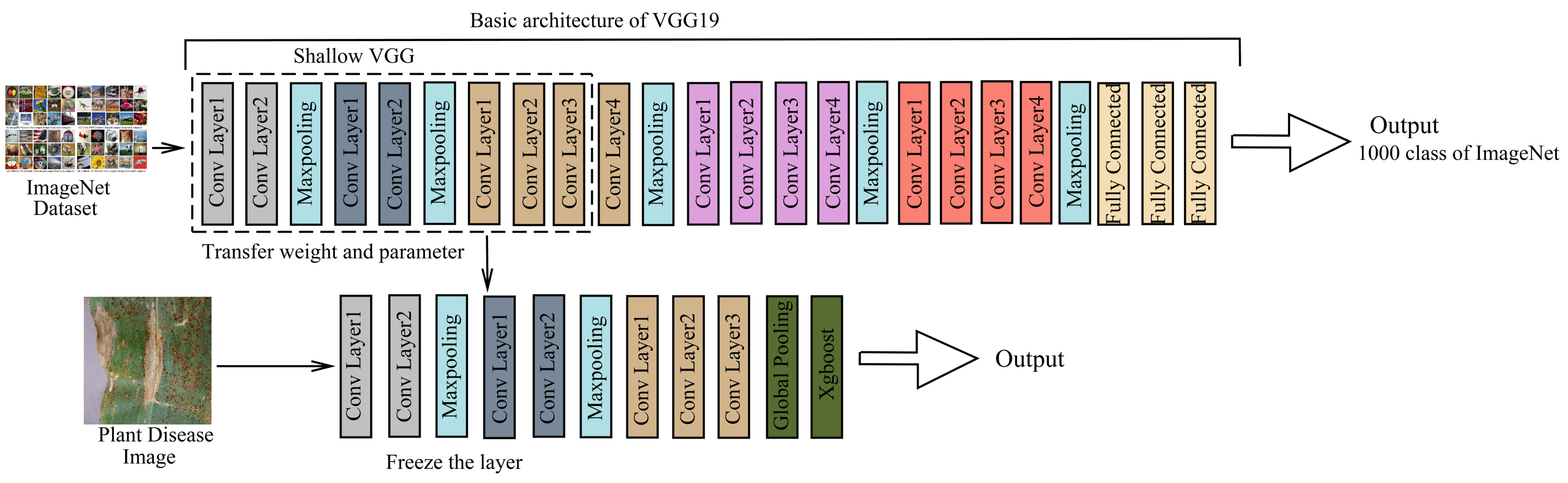
In this paper, we have proposed two models namely: shallow VGG with Xgboost, shallow VGG with RF to identify the diseases in plants. VGG19 is considered as the base model of the network.

•

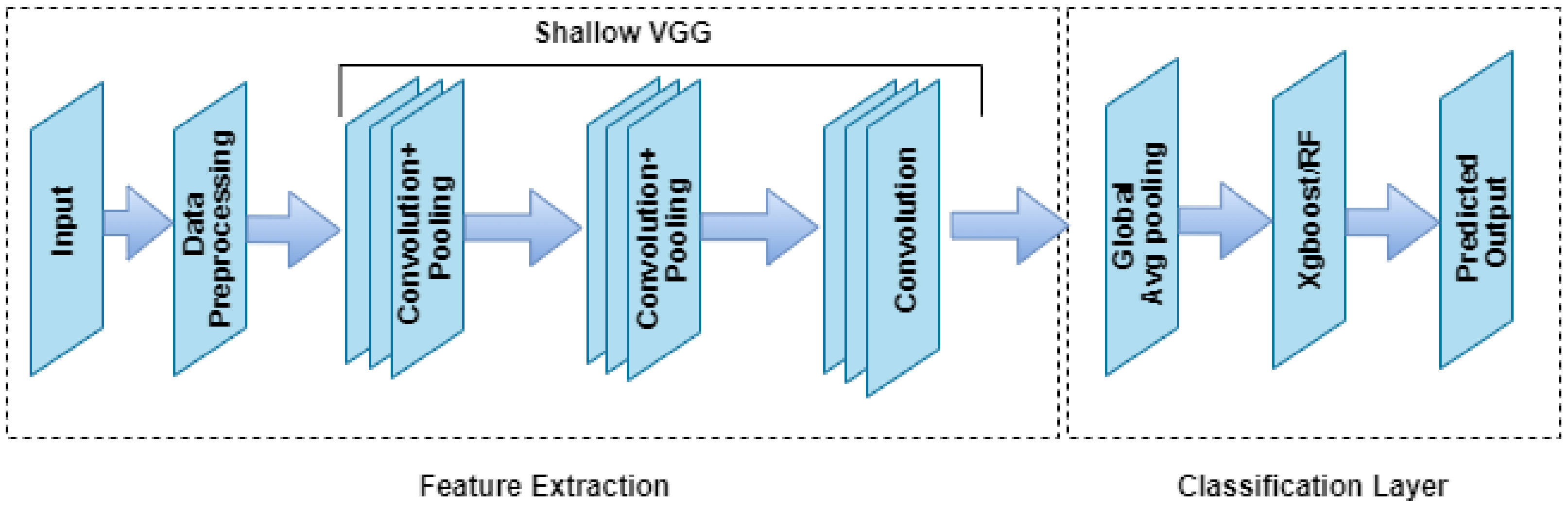
The implemented network consists of only nine layers of VGG network with a global average pooling layer. It differs from the original VGG19 network with no fully connected layers in the network. This simply reduces the number of the parameter by a huge margin. We found that shallow VGG network with machine learning classifier performs well and shallow VGG with Xgboost classifier outperforms original VGG19.

•

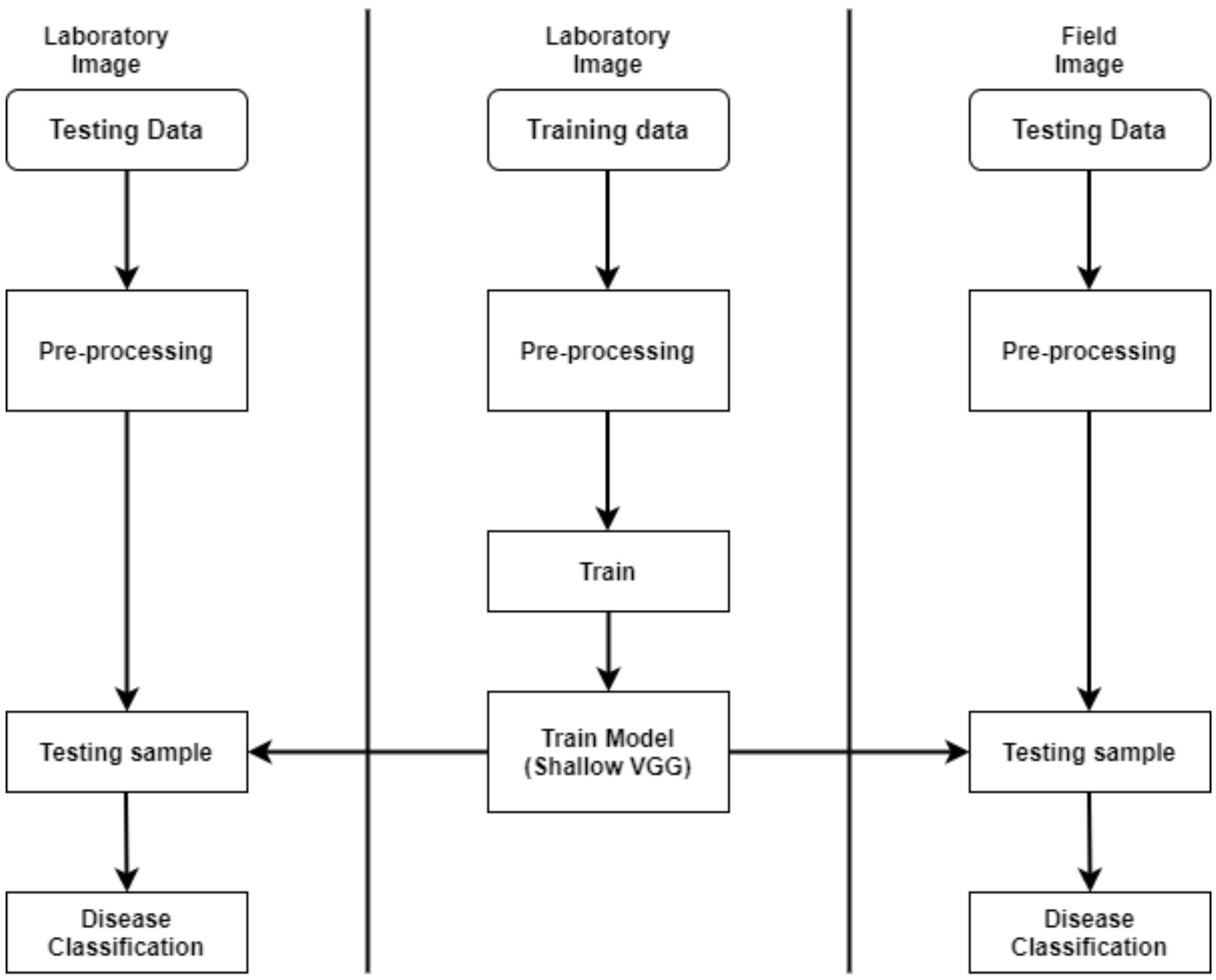
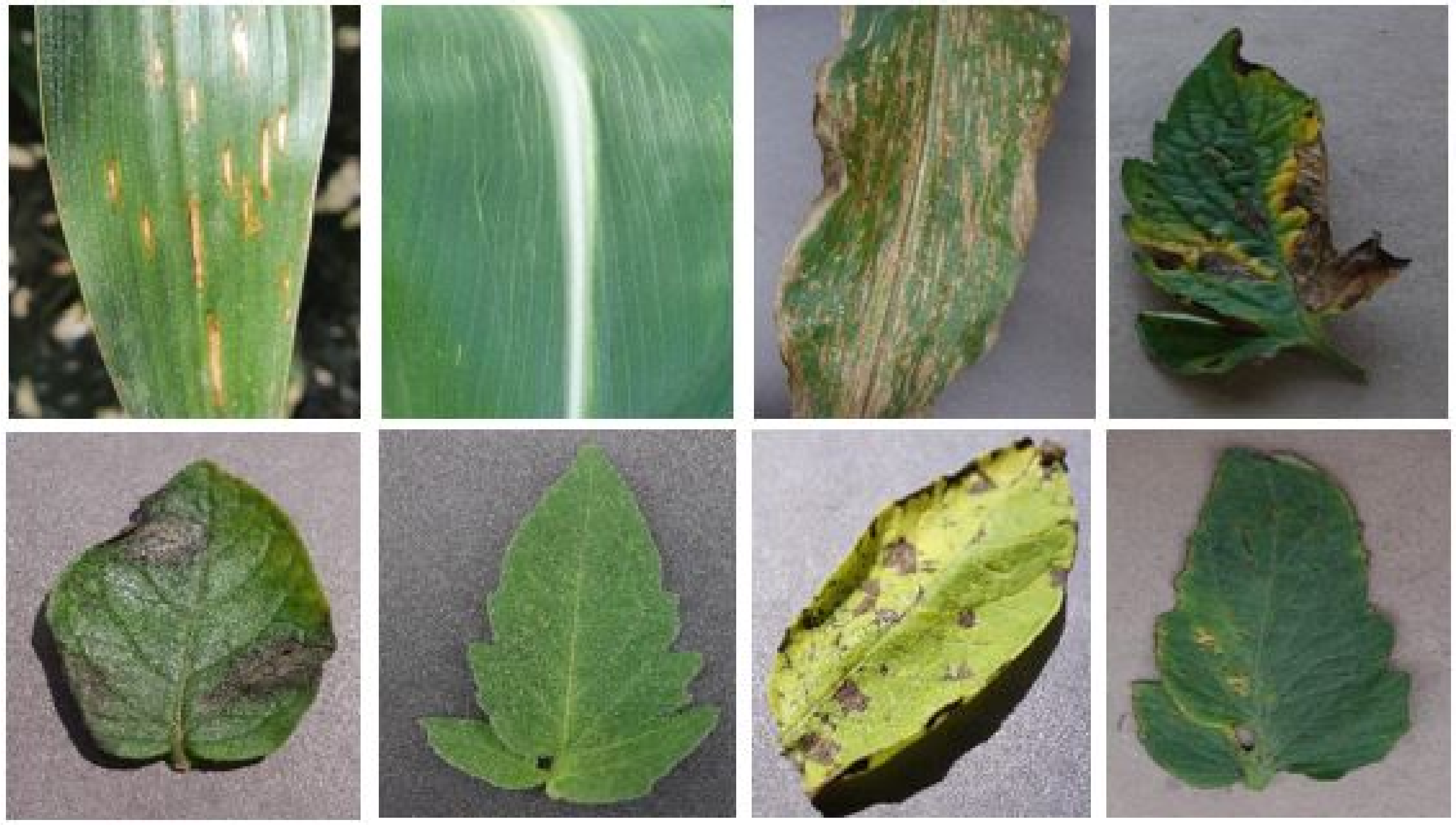
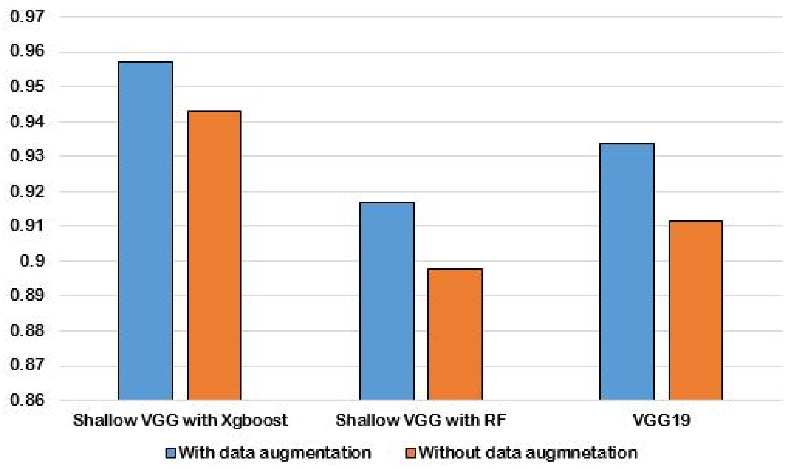
Instead of using only laboratory images, we have measured the model performances with both laboratory and field conditioned images.

•

We have done an extensive experiment on the proposed model and find that, the proposed model has an advantages in accuracy, precision, recall, and f1-score. Finally, a comparative analysis of the implemented model, with other deep learning models, and traditional hand-crafted based approaches is carried out.

The rest of the paper is organized as follows: Section 2 gives brief discussions about the related work along with their limitations. Section 3 discussed the materials and methodology. Experimental results, as well as the comparative analysis, are provided in Section 4. Finally, Section 5 concludes the paper with future scope.

2. Related Work

In this section, we are going to discuss on the brief overview of the work done so far in identification of plant diseases. In the field of agriculture, two methodologies are used extensively to classify the diseases: first one is a traditional hand-crafted feature-based and second one is deep learning feature-based. Recent works focus mainly on the development of deep learning-based models such as CNN which has the ability to learn the features automatically. Mohanty et al. [26] used AlexNet and GoogleNet model for classifying 14 crop species and 26 crop diseases. Ferentinos et al. [1] used five different CNN architectures: AlexNet, AlexNetOWTBn, GoogLeNet, OverFeat, and VGG, to identify 58 distinct classes and achieved the highest accuracy of 99.53% using VGG architecture. The testing dataset used in this work to evaluate the performances of the models was part of the same dataset that was used to train the model. The performance drops significantly when the model is trained on laboratory images and tested on real field images. Geetharamani et al. [27] used a nine-layer deep CNN architecture to identify different plant diseases in the Plant Village dataset and achieved an accuracy rate of 96.46%. Extension of their work includes, collecting images from various sources of different plants, different geographic areas, cultivation conditions, etc.

Amara et al. [28] used LeNet architecture to identify banana diseases under challenging conditions such as complex background, illumination, and different orientations. Modified AlexNet architecture was used by Liu et al. [29] to identify four different apple diseases and they achieved an accuracy rate of 97.62% which was higher than the traditional approach. As a future work, the authors suggested detecting apple leaf diseases in real-time conditions and with more types of apple diseases. The authors also suggested using Faster RCNN (Regions with Convolutional Neural Network), YOLO (You Only Look Once), and SSD (Single Shot MultiBox Detector) to identify the diseases.

Fuentes et al. [30] identified tomato diseases using Faster Region-based Convolutional Neural Network (Faster R-CNN), Region-based Fully Convolutional Network (R-FCN). They tested their model with several class variations and with complex backgrounds. Brahimi et al. [31] made an effort to enhance the performance of two popular deep learning models namely AlexNet and GoogleNet for identification of tomato leaf diseases. Reduction of the computation time and size of deep learning models for small devices was an important issue regarding their approach.

Yang Li [16] focused on designing a simple CNN network by considering limited computation resources and identified the cotton pest. It was achieved an accuracy rate of 95.4%. Triplet loss function was used in their approach. PD2SE-Net used by Liang et al. [32] to diagnose the diseases in plant and severity estimation of the diseases. The network used ResNet50 as a base model with shuffle unit as an auxiliary structure. Though It achieved a satisfactory performance accuracy, the parameter generated in this model is much higher, which implied the higher computational cost.

Johannes et al. [33] identified four different wheat diseases based on hot spot region. After extraction of the hot-spot region, they categorized each region based on visual characteristics. Meta classifier was used in this approach to classify the diseases. Exact extraction of diseased region is an important issue in this work. Picon et al. [34] extended the work and identify these crop diseases using Residual Network (ResNet50). Yang Lu et al. [13] proposed a small six layer deep CNN based on LeNet and AlexNet model to identify 10 different rice diseases. Choosing the optimal number of layers and neuron size is one of the challenging issues in their deep CNN model. Different deep CNN models were used by Sethy et al. [35] to identify four different rice diseases. In their paper, they extracted the features from the deep learning models and classified them using an SVM classifier.

In a recent study, Barbedo et al. [36] considered lesions of the leaf instead of using the whole leaf to identify the diseases. They achieved reliable results however the segmentation of the lesion region is performed manually.

Pre-trained VGG net on ImageNet data with two inception module used in [37] to identify rice diseases and achieved an accuracy of 92%. As VGG network itself generates a large number of parameters, adding more layers to this network may increase parameters drastically. Therefore the computation cost was more. Shallow CNN-based approach used in [3] to identify maize, apple, and grape diseases. After the extraction of features, they reduced the features using Principal Component Analysis (PCA) and classified using SVM and RF and achieved accuracy in between 91–94%. While reducing the features, some of the important features may be removed which affected the performance of this work.

Self-Attention Convolutional Neural Network (SACNN) based approach used by Zeng et al. [38] to identify different crop leaf diseases. The network used in this work consists of basic network (Base Net) which extracted the global features and the self-attention (SA) network extracted the local features of the lesion area. The key issue of SACNN based approach is keeping SA network in proper places of the Base-Net so that the model works properly for the identification of crop diseases.

3. Materials and Methods

A generalized overview of the identification of plant diseases using shallow VGG is presented in Figure 1. To implement our proposed work, firstly, the images of diseased leaves of corn, tomato, and potato are collected from the Corn [39] and PlantVillage [26] dataset as well as from the field. Then the images are labeled according to the disease classes based on expert knowledge in case of field images. After that, pre-processing of images is performed which includes resizing of images, filtering of images, and different data augmentation techniques such as rotation, flipping, zca whitening, and shifting to increase the dataset size. The training and the testing images are fed into the shallow VGG model and the features are extracted. At last, we have used two different machine learning classifiers to classify the diseased leaf images. A detailed description of the implemented models is discussed in subsequent sub-sections.

3.1. Convolutional Neural Network

Convolutional Neural Network (CNN) is a deep learning technique used mainly in recognition and classification purposes. In comparison with hand-crafted traditional approaches, CNN has the potential to perform better. It has the ability to learn the robust features directly from the input images. Whereas, to classify in the traditional hand-crafted feature-based approach, we need to extract the features separately. Different popular deep CNN models are used in identification of plant diseases such as AlexNet [40], VGG net [20,41], InceptionV3 [14,42], ResNet50 [35], DenseNet [35], etc. From the research, it is shown that deep CNN-based models can achieve better performance accuracy in identification of plant diseases. Typically a CNN consist of convolutional layer, pooling layer, and fully connected layer [13].

The convolutional layer is the main component in CNN, which extracts the features of the input images using different convolutional kernel. The output of the convolutional operation is computed as:

$$x_j=I*W_j+b_{j}wherej=1,2,\dots \dots F$$

(1)

here, $x_j$ is the output feature corresponds to jth convolution filter, $W_j$ is the corresponding weight, $b_j$ is the bias and F is the number of filter.

Poling layer down-samples the input vector and avoids over-fitting in the output. The pooling layer reduces the computational complexity of the model. The output of the pooling layer is evaluated as:

$$x_i^k=down(x_i^{k-1},s)$$

(2)

where $down\left(\right)$ represents the downsample, $x_i^{k-1}$ represents the feature vector of previous layer and s represents the pool size. Max pooling and average pooling are two commonly used pooling operation.

After the convolutional and pooling layer, several fully connected layers are there which transform the output of the previous layer to a single column vector. Usually, softmax function is used for multi-class prediction. Dropout regularization is used to decrease the neuron size and to avoid over-fitting. The softmax function is written as:

$$softmax\left(z_j\right)=\frac{e^{z_j}}{{\sum }_k^K{e}^{z_k}}for(j=1,2,\dots \dots K)$$

(3)

where K represents the dimension of z vector.

3.2. Visual Geometry Group (VGG19)

In recent times, several popular deep learning models such as AlexNet, VGGNet, ResNet, Inception, DenseNet, Xception, etc., have been used in the identification of plant diseases. Among this model, VGG is a relatively simple network developed by Simonyan and Zisserman [20]. VGG network consists of several convolution layer and pooling layer with different numbers of filter. VGGNet has two models VGG16 and VGG19. VGG16 consists of 16 convolutions and pooling layer with fully connected layer. VGG19 consist of 19 convolutions and pooling layer with fully connected layer. The number of parameters generated in the VGG network is 140 million. The VGG network is pre-trained on a large dataset (ImageNet) with 1000 categories.

In our work, we have used shallow VGG model which takes nine layers of the VGG19 model that includes 7 convolution layer and 2 max-pooling layer. The input size used in our implemented model is $256\times 256\times 3$ and after performing the convolution and pooling operation the output size is $64\times 64\times 256$. Instead of a fully connected layer, we have used global average pooling layer which reduces the number of parameters and dropout layer. The dropout layer plays an important role in reducing the overfitting problem of the network. After extracting the features using Shallow VGG, we have classified them using Random forest and Xgboost classifier. The parameter generated in our implemented model is 1.73 million which is much lesser in comparison with the original VGG19 model.

Table 1. Related parameter and output size of original VGG19 model.

Layers	Kernel Size	Output Size	Parameter
Input	-	(256, 256, 3)	-
$Block{1}_{-}conv1$	3 × 3	(256, 256, 64)	1792
$Block{1}_{-}conv2$	3 × 3	(256, 256, 64)	36,928
$Block{1}_{-}pool$	2 × 2	(128, 128, 64)	-
$Block{2}_{-}conv1$	3 × 3	(128, 128,128)	73,856
$Block{2}_{-}conv2$	3 × 3	(128, 128, 128)	147,584
$Block{2}_{-}pool$	2 × 2	(64, 64, 128)	-
$Block{3}_{-}conv1$	3 × 3	(64, 64, 256)	295,168
$Block{3}_{-}conv2$	3 × 3	(64, 64, 256)	590,080
$Block{3}_{-}conv3$	3 × 3	(64, 64, 256)	590,080
$Block{3}_{-}conv4$	3 × 3	(64, 64, 256)	590,080
$Block{3}_{-}pool$	2 × 2	(32, 32, 512)	-
$Block{4}_{-}conv1$	3 × 3	(32, 32, 512)	1,180,160
$Block{4}_{-}conv2$	3 × 3	(32, 32, 512)	2,359,808
$Block{4}_{-}conv3$	3 × 3	(32, 32, 512)	2,359,808
$Block{4}_{-}conv4$	3 × 3	(32, 32, 512)	2,359,808
$Block{4}_{-}pool$	2 × 2	(16, 16, 512)	-
$Block{5}_{-}conv1$	3 × 3	(16, 16, 512)	2359808
$Block{5}_{-}conv2$	3 × 3	(16, 16, 512)	2,359,808
$Block{5}_{-}conv3$	3 × 3	(16, 16, 512)	2,359,808
$Block{5}_{-}conv4$	3 × 3	(16, 16, 512)	2,359,808
$Block{5}_{-}pool$	2 × 2	(8, 8, 512)	-
Global Average Pooling	-	(512)	-

and

Table 2. Related parameter and output size of shallow VGG model.

Layers	Kernel Size	Output Size	Parameter
Input	-	(256, 256, 3)	-
$Block{1}_{-}conv1$	3 × 3	(256, 256, 64)	1792
$Block{1}_{-}conv2$	3 × 3	(256, 256, 64)	36,928
$Block{1}_{-}pool$	2 × 2	(128, 128, 64)	-
$Block{2}_{-}conv1$	3 × 3	(128, 128,128)	73,856
$Block{2}_{-}conv2$	3 × 3	(128, 128, 128)	147,584
$Block{2}_{-}pool$	2 × 2	(64, 64, 128)	-
$Block{3}_{-}conv1$	3 × 3	(64, 64, 256)	295,168
$Block{3}_{-}conv2$	3 × 3	(64, 64, 256)	590,080
$Block{3}_{-}conv3$	3 × 3	(64, 64, 256)	590,080
Global Average Pooling	-	(256)	-

show the parameter generated on VGG19 and shallow VGG model, respectively.

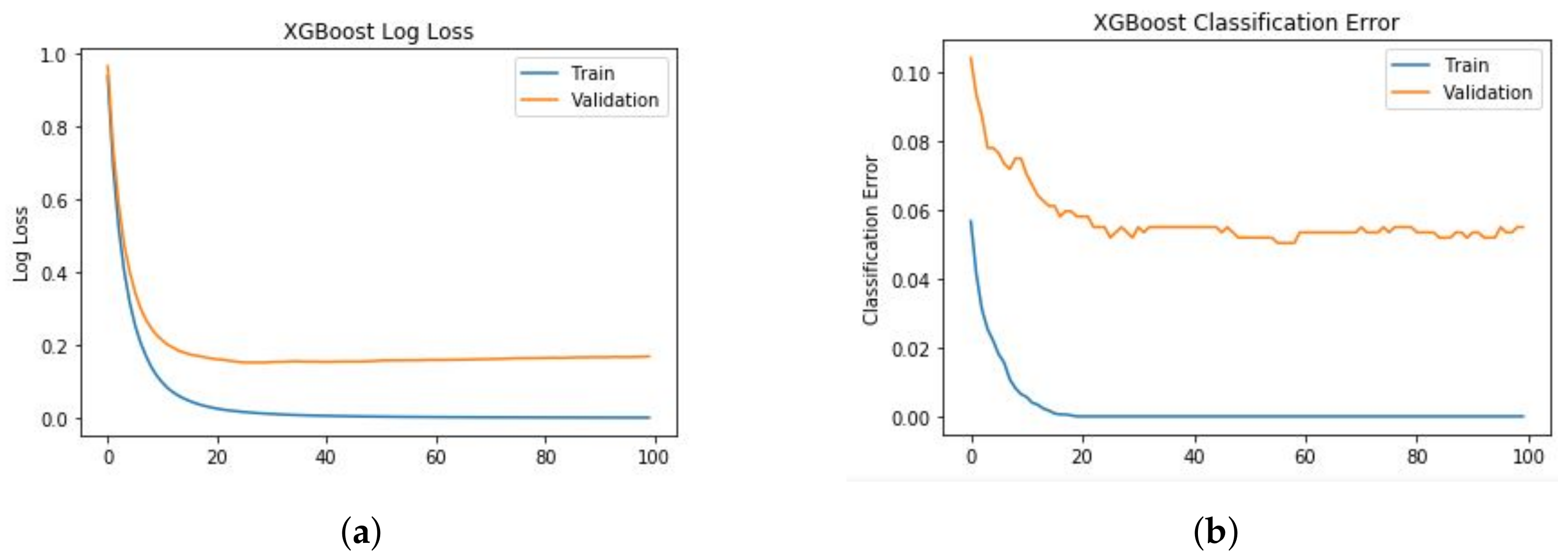
3.3. Extreme Gradient Boosting (Xgboost)

Xgboost is a decision tree based ensemble learning algorithm designed by Chen and Guestrin. It is used mainly in classification and regression problem [43]. It uses gradient boosting framework. In prediction of unstructured data it outperforms all other classification algorithm. The final prediction of the output can be represented as:

$${\widehat{y}}_i=\phi \left(x_i\right)=\sum _{k=1}^K{f}_k\left(x_i\right),f_kϵF,$$

(4)

where the $x_i$ are the training set and their corresponding class labels is represented by $y_i$. $f_k$ is the leaf score for the kth tree and F is the set of all K scores for all regression trees. Regularization is applied in Xgboost to improve the result.

$$\mathcal{L}\left(\phi \right)=\sum _{i}l({\widehat{y}}_i,y_i)+\sum _k\Omega \left(f_k\right)$$

(5)

The term l in Equation (5) represents the loss function which signifies how well the model fit into the training data. Loss function is the squared difference between predicted output $\widehat{y_i}$ and actual output $y_i$. The term $\Omega$ represents the regularization which measures the complexity of the tree. Optimizing the regularization encourages generalized simpler model and avoids overfitting.

$$\Omega \left(f\right)=\gamma T+\frac{1}{2}\lambda \sum _{j=1}^T{w}_j^2$$

(6)

Regularization uses two parameter. T is the number of leaves in ith tree and w defines the weight in each leaves. $\gamma$ and $\lambda$ are constants that controls the degree of regularization.

$${\mathcal{L}}^{\left(t\right)}\simeq \sum _{i=1}^n\left[l(y_i,{\widehat{y}}^{(t-1)})+g_i{f}_t\left(x_i\right)+\frac{1}{2}{h}_i{f}_t^2\left(x_i\right)\right]+\Omega \left(f_t\right)$$

(7)

The $g_i$ indicates the first order differentiation $g_i={\partial }_{\widehat{y}(t-1)}{(y_i-{\widehat{y}}^{(t-1)})}^2$ and $h_i$ indicates the second order differentiation $h_i={\partial }_{\widehat{y}(t-1)}^2{(y_i-{\widehat{y}}^{(t-1)})}^2$. After removing the constant term the simplified objective at step t is represented as:

$$\begin{array}{cc}\hfill {\tilde{\mathcal{L}}}^{\left(t\right)}& \simeq \sum _{i=1}^n\left[g_i{f}_t\left(x_i\right)+\frac{1}{2}{h}_i{f}_t^2\left(x_i\right)\right]+\Omega \left(f_t\right)\hfill \\ \hfill & =\sum _{i=1}^n\left[g_i{f}_t\left(x_i\right)+\frac{1}{2}{h}_i{f}_t^2\left(x_i\right)\right]+\gamma T+\frac{1}{2}\lambda \sum _{j=1}^T{w}_j^2\hfill \\ \hfill & =\sum _{j=1}^T\left[\left(\sum _{iϵI_j}{g}_i\right)w_j+\frac{1}{2}(\sum _{iϵI_j}{h}_i+\lambda )w_j^2\right]+\gamma T\hfill \end{array}$$

(8)

where $I_j=\left\{i\left|q\right(x_i)=j\right\}$ defines the instance set of leaf j. For a given fixed tree structure q(x), the optimal weight $w_j^{*}$ of each leaf j is computed as:

$$\begin{array}{cc}\hfill \frac{d{L}^t}{d{w}_j^{*}}& =0\hfill \\ \hfill w_j^{*}& =-\frac{{\sum }_{iϵI_j}{g}_i}{{\sum }_{iϵI_j}{h}_i+\lambda }\hfill \end{array}$$

(9)

and evaluated the corresponding optimal value as:

$${\tilde{\mathcal{L}}}^{\left(t\right)}\left(q\right)=-\frac{1}{2}\sum _{j=1}^T\frac{{\left({\sum }_{iϵI_j}{g}_i\right)}^2}{{\sum }_{iϵI_j}{h}_i+\lambda }+\gamma T$$

(10)

Finally a greedy algorithm is used which starts from node 0 to build the tree. Assuming that $I_L$ is the instance set of left node and $I_R$ is the instance set of right node after the split and $I=I_L\cup I_R$, the loss reduction after split can be mathematically represented as:

$${\mathcal{L}}_{split}=\frac{1}{2}\left[\frac{{\left({\sum }_{iϵI_L}{g}_i\right)}^2}{{\sum }_{iϵI_L}{h}_i+\lambda }+\frac{{\left({\sum }_{iϵI_R}{g}_i\right)}^2}{{\sum }_{iϵI_R}{h}_i+\lambda }-\frac{{\left({\sum }_{iϵI}{g}_i\right)}^2}{{\sum }_{iϵI}{h}_i+\lambda }\right]-\gamma$$

(11)

3.4. Random Forest (RF)

Random forest [44] is a decision tree based supervised machine learning algorithm used for classification and regression problem. RF generates multiple decision trees using randomly selected subset of training data. Because of high classification accuracy, RF is more popular in classification problems. Growing the forest depends on the number of tree generated. It is a user defined function. The generated trees have high variance and low bias [44]. The final prediction is made by averaging all the class probabilities from the trees [45]. The new test sample is evaluated against the trees in the ensemble and each tree voted for a class. The class with the maximum votes will be the final predicted output.

3.5. Proposed Approach

As mentioned, Visual Geometry Group (VGG) is a widely used deep learning model amongst all the models and also highly portable in nature. Though VGG is a simple architecture with convolution and pooling layers, the number of parameters generated in the VGG network is relatively high and it is more than 140 million. The VGG network is pre-trained on a large dataset (ImageNet) with 1000 categories. In [3] the author showed that instead of using a large deep network, shallow CNN provide enough feature information to classify. Instead of training the model with randomly initialized weights, we have used the pre-trained network which is trained on a large dataset. Figure 2 shows the VGG19 model and in our work, we have used only 7 convolution and 2 pooling layers from the pre-trained network. VGG19 is considered the base model. After the 7th convolution layer, we have replaced all convolution layer, pooling layer, and fully connected layer with the Global Average Pooling layer and Batch Normalization layer. The modified VGG19 network is named as shallow VGG network.

Firstly, the images of plant leaves are pre-processed and fed into the shallow VGG network. The input size used in our model is $256\times 256\times 3$. The convolution layers of the network extract the features and pooling layers are used to reduce the dimension of the features. Instead of using a fully connected layer on top, we have used global average pooling. Global average pooling has an advantage over a fully connected layer is that it is more familiar to the convolution structure. Another advantage is that overfitting can be avoided in the global average pooling layer since there is no parameter to optimize [46]. The model first extracts the features by $3\times 3$ convolution with 64 filters. Next, $2\times 2$ max-pooling is used which reduces the feature dimension and computation. Next $3\times 3$ convolution is used with 128 filter to extract the features. The second $2\times 2$ max-pooling layer further reduces the feature dimension. The third block of convolutional layer uses $3\times 3$ convolution and 256 filter. At last global average pooling layer is used and it generates 256 neurons which is used for classification. Later, dropout is used to reduce over-fitting and also to improve the generalization of the model. After that classification of the diseased leaves are performed using Random forest and Xgboost classifier. Figure 3 shows the proposed model used in the identification of plant diseases. The parameter used in this shallow VGG network is shown in Table 2.

The shallow VGG model has two parts. one part is using this shallow network to extract the features and the next part is used to classify using two classical machine learning classifiers such as random forest and Xgboost classifier. The shallow VGG reduces the parameter by a large margin. Hence, the computational cost of this model is much less in comparison to the VGG19 model.

4. Results and Discussion

4.1. Experiment Setup

In our experiment, all the pre-processing, CNN based feature extraction and classification are performed in Anaconda-python 3.6 with jupyter notebook environment. The model is implemented using keras-libray, OpenCV-python3 library, etc. The experiment is conducted on Intel(R) Core (TM) i7-6700 CPU at 3.40 GHz with 8 GB memory.

4.2. Data Acquisition

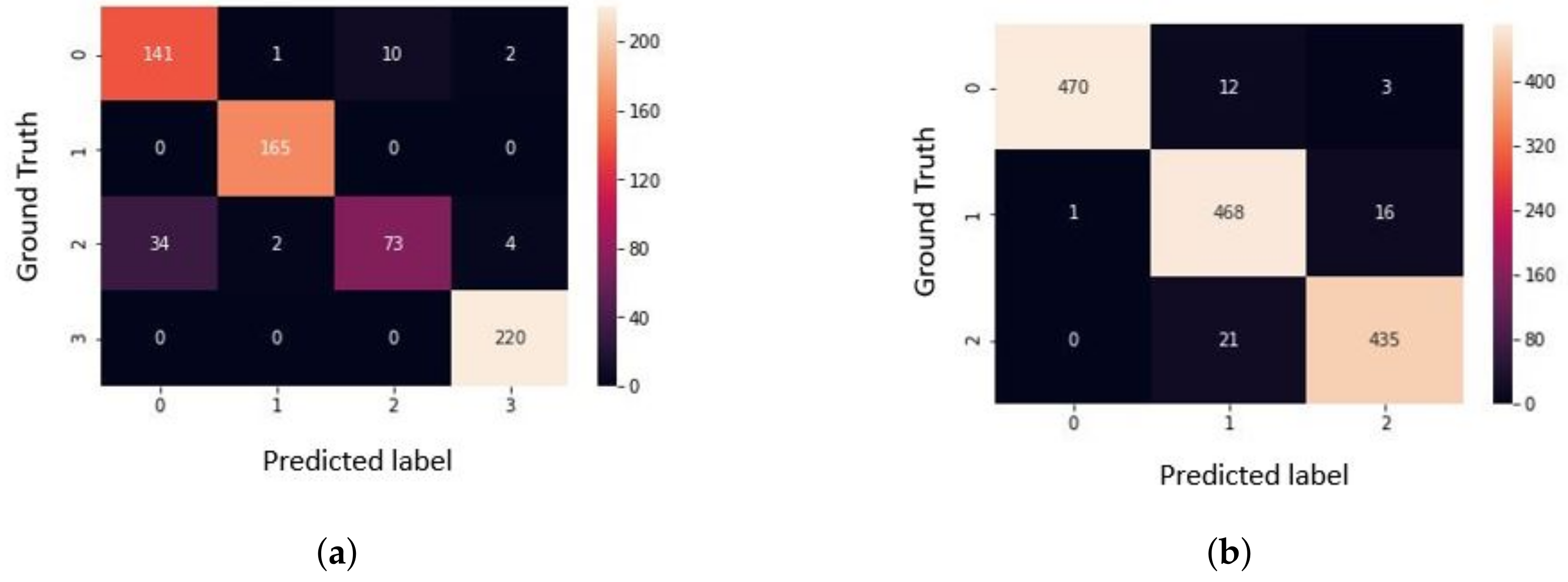
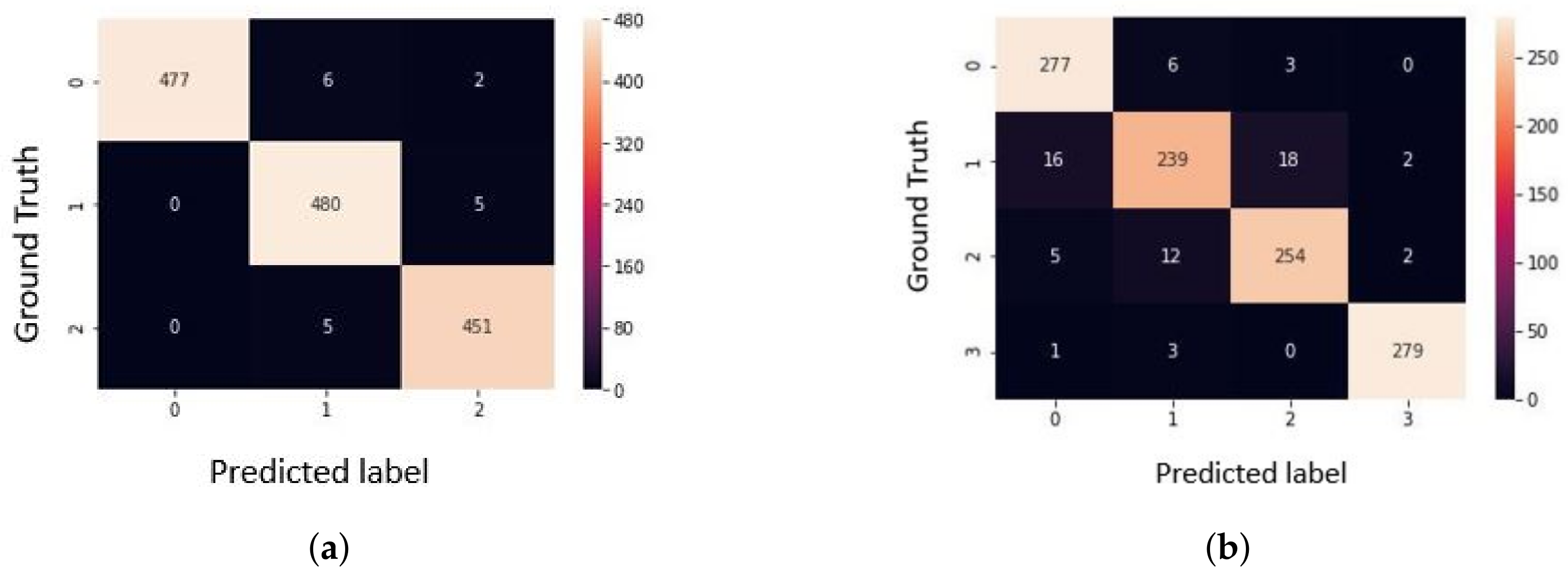
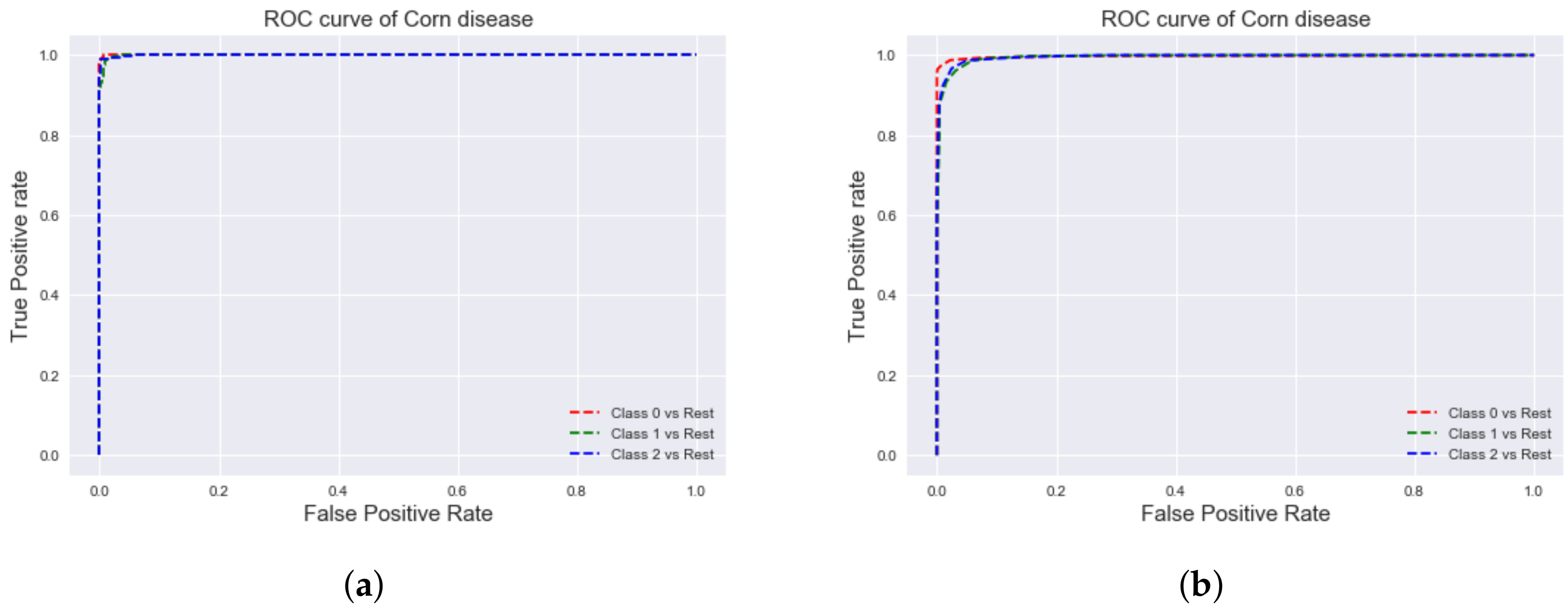
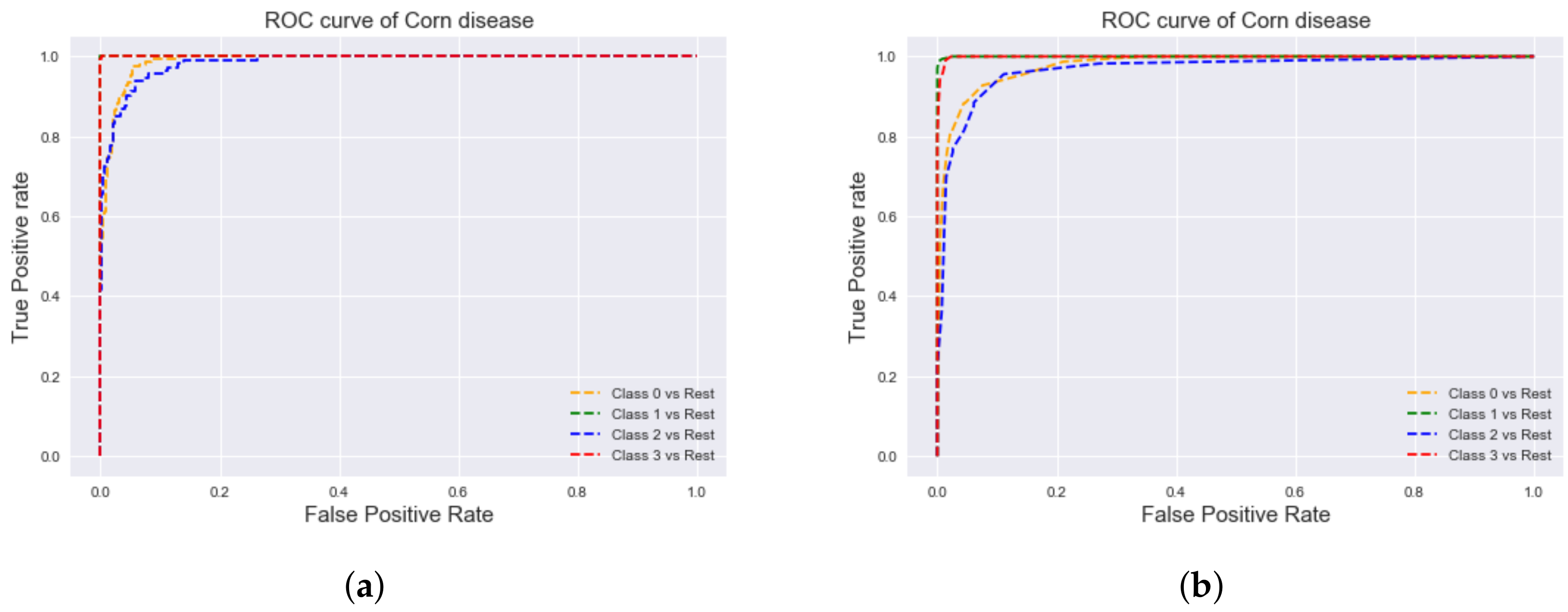
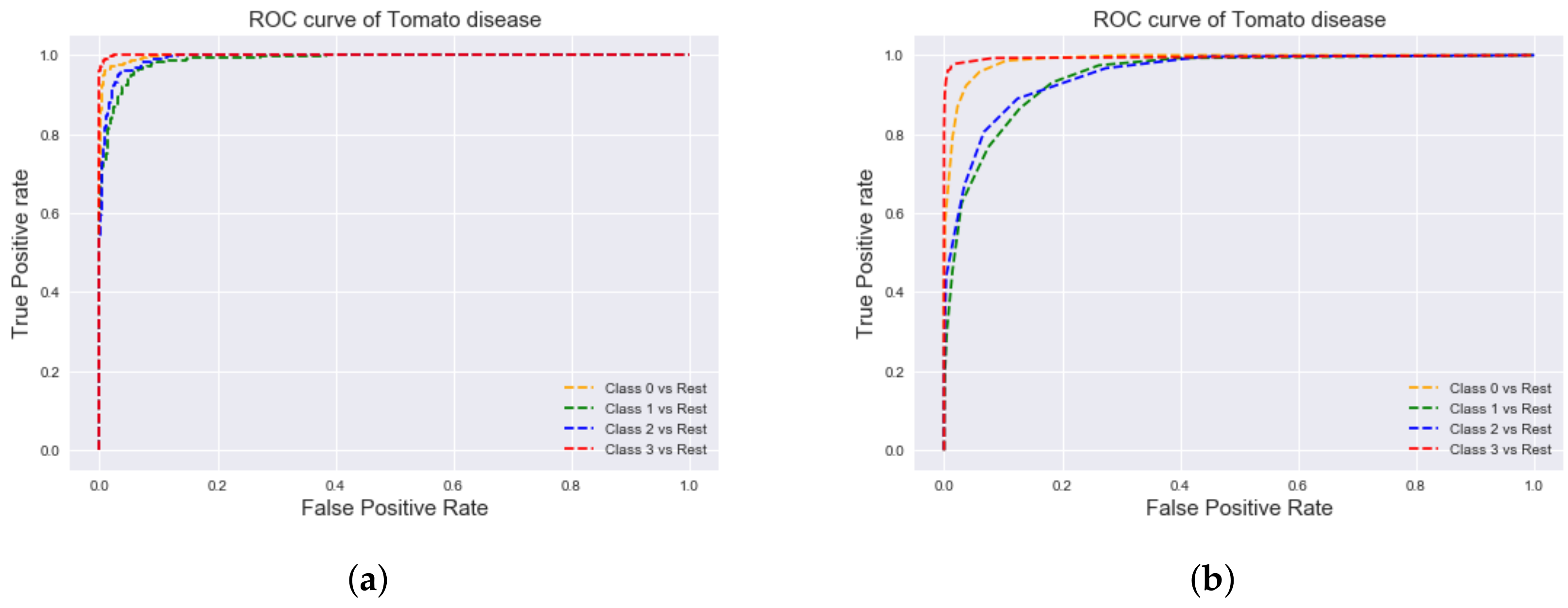
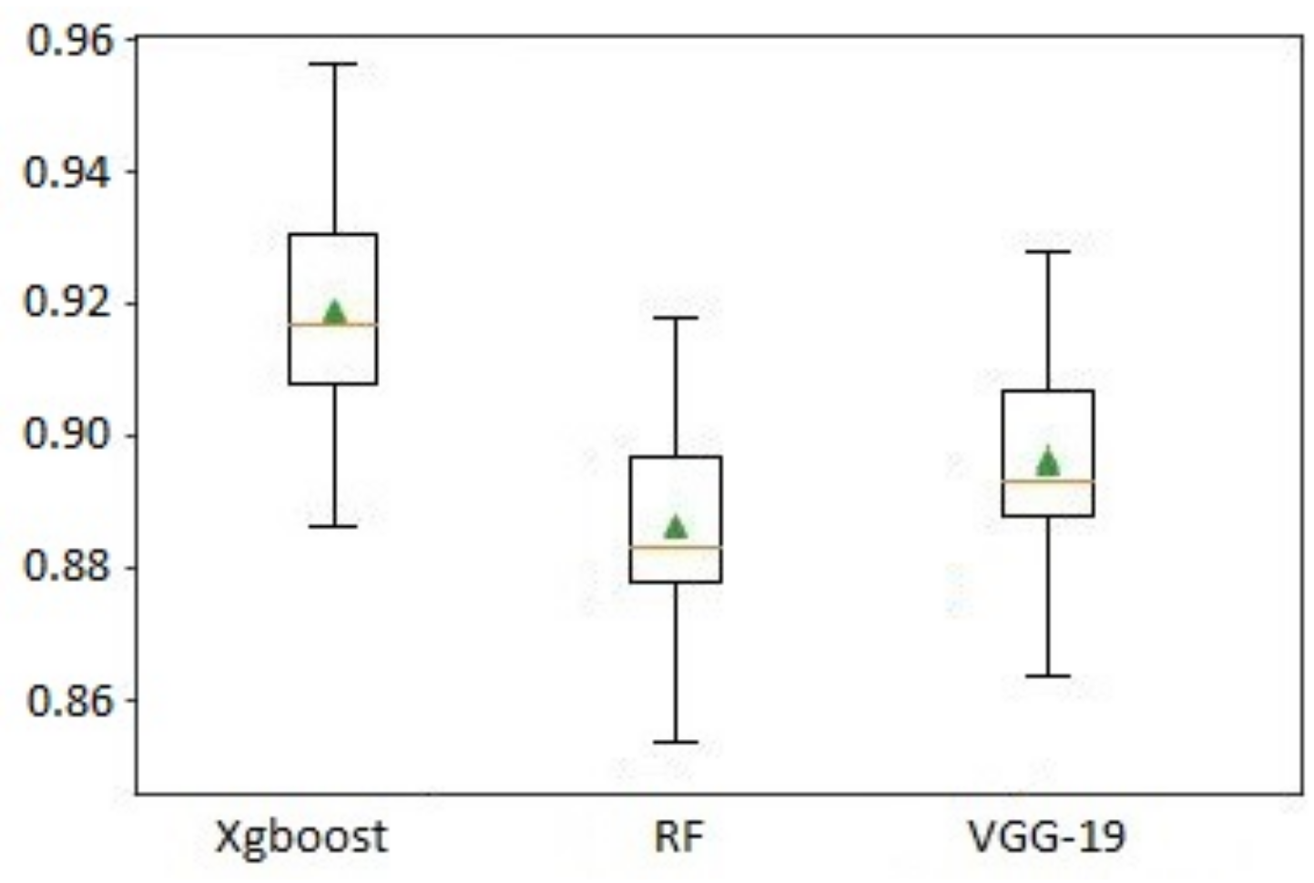
In this work, we have used publicly available corn dataset [39] and PlantVillage [26] open dataset. From the PlantVillage dataset specially potato and tomato leaf diseases are considered. The corn dataset consists of 4188 images of four different categories diseases namely Blight, Common rust, healthy, Gray leaf spot. Potato leaf images consist of 7128 images of 3 categories of diseases, such as early blight, late blight, and healthy images. Tomato leaf images consist of 7399 images of four different categories of diseases, such as bacterial spot, early blight, healthy, and late blight images. Moreover, some field conditioned images captured under non-uniform illumination. Field background conditioned images are taken using smartphone from Shillong, India, region and are also used to train the network and to evaluate the performances. The captured images are labeled according to the class name of the diseases. While capturing the image, images are captured in such a way that the image contains the region of interest. Different data augmentation techniques such as flipping, rotation, horizontal and vertical shifting, zca whitening are used to increase the number of images in the dataset as deep learning requires large volume of data to obtained better outcome [27]. The images are pre-processed and resized to $256\times 256$ pixel to fit in the model. The dataset is splitted randomly in the ratio of 80% training and 20% testing ratio.

Table 3. Dataset description.

Name of the Dataset	Class	Images in Dataset	Train Images	Test Images	Field Images	Total
Corn disease data	4	4188	3350	838	312	4500
Potato disease data	3	7128	5702	1426	570	7698
Tomato disease data	4	7399	5919	1480	423	7822

summarizes the dataset used along with the number of images in the actual dataset and images captured in field condition. Some samples of these datasets are shown in Figure 4.

4.3. Results

To evaluate the performances of the implemented model, we have used different performance measure metrics such as accuracy, precision, recall, specificity, and f1-score. To evaluate these metrics we need several indices such as True Positive (TP), False Positive (FP), True Negative (TN), and False Negative (FN). TP is the correctly classified images in a particular category. FP is the number of wrongly classified images, whereas TN is the sum of the correctly classified images in all other categories and FN is the number of misclassified images from the relevant category. The performance metrics are calculated using the following equations

$$Accuracy=\frac{\mathrm{TP}+\mathrm{TN}}{\mathrm{TP}+\mathrm{FP}+\mathrm{TN}+\mathrm{FN}}$$

(12)

$$Precision=\frac{\mathrm{TP}}{\mathrm{TP}+\mathrm{FP}}$$

(13)

$$Recall=\frac{\mathrm{TP}}{\mathrm{TP}+\mathrm{FN}}$$

(14)

$$Specificity=\frac{\mathrm{TN}}{\mathrm{TN}+\mathrm{FP}}$$

(15)

$$f1-score=\frac{2\times precision\times recall}{precision+recall}$$

(16)

Table 4. Performance comparison of the implemented models.

Dataset	Parameter	Shallow VGG-Xgboost	Shallow VGG-RF	VGG-Softmax
Corn	Precision	0.9298	0.8904	0.8942
	Recall	0.9345	0.9102	0.8756
	F1-score	0.9321	0.9002	0.8849
	Accuracy	0.9447	0.9201	0.8961
	Parameter	1,735,488	1,735,488	20,173,700
Potato	Precision	0.9875	0.9626	0.9767
	Recall	0.9907	0.9634	0.9771
	F1-score	0.9890	0.9630	0.9769
	Accuracy	0.9874	0.9628	0.9772
	Parameter	1,735,488	1,735,488	20,173,700
Tomato	Precision	0.9384	0.8658	0.9291
	Recall	0.9388	0.8678	0.9354
	F1-score	0.9385	0.8668	0.9322
	Accuracy	0.9391	0.8675	0.9279
	Parameter	1,735,488	1,735,488	20,173,700

shows the performances of the implemented models. From Table 4, it can be observed that Shallow VGG with Xgboost has better performance in all the indices such as precision, recall, f1-score, and accuracy. The accuracy obtained in shallow VGG with Xgboost is 0.9447, 0.9874, 0.9391 in corn, potato, and tomato, respectively. The values obtained in all indices using Shallow VGG with Xgboost is far better than the shallow VGG with RF and VGG19 model. Moreover, the number of the parameters is also important which determines the computational cost of the model. From Table 4, it can be seen that the number of parameter used in our implemented shallow VGG model is much less as compared with the original VGG19 model. Our implemented Shallow VGG network uses only 8% of the total parameter as compared to the VGG19 model.

Figure 5, Figure 6 and Figure 7 are the confusion matrix of the three different plant species(corn, potato, tomato) for shallow VGG with RF and shallow VGG with Xgboost, respectively. It is seen that both the model perform well but from Figure 6b and Figure 7a,b shows significant improvement using shallow VGG with Xgboost. Misclassified sample reduces from 34 in Figure 5a to 18 in Figure 6b in corn diseases. Still, the maximum misclassified class belongs to class 2. In the case of tomato diseases, misclassified sample reduces from 33 in Figure 6a to 16 in shallow VGG with Xgboost as shown in Figure 7b. Both the model performs well in identification of healthy classes.

We evaluated the performances of the model for each dataset separately. Figure 6b shows the prediction results of corn diseases and its corresponding performances for each class are shown in

Table 5. Performance evaluation of individual classes of corn diseases using VGG and Xgboost.

Disease Class	Precision	Recall	Specificity
Blight	89.61	88.46	96.77
Common rust	100.00	99.39	100.00
Grey leaf spot	82.30	87.73	96.33
Healthy	100.00	98.21	100.00
Average	92.98	93.45	98.27

. It is seen that 18 samples of “grey leaf spot” diseases are classified as “blight” diseases. Out of 652 images, 616 images are predicted correctly in shallow VGG with Xgboost. From Table 5, it is seen that the average precision, recall, and specificity obtained is 92.98%, 93.45%, and 98.27%, respectively. Figure 7a shows the prediction results of potato diseases and amongst the three plants, the implemented model achieves the highest accuracy rate of 98.74% in potato disease detection. On the other hand, the performance accuracy of tomato disease identification is a little bit lesser in comparison with corn and potato. The average accuracy obtained in tomato disease identification is 93.91%. From Table 5,

Table 6. Performance evaluation of individual classes of potato diseases using VGG and Xgboost.

Disease Class	Precision	Recall	Specificity
Early blight	98.35	100.0	99.15
Late blight	98.96	98.76	99.46
Healthy	98.90	98.47	99.48
Average	98.74	99.07	99.36

and

Table 7. Performance evaluation of individual classes of Tomato diseases using VGG and Xgboost.

Disease Class	Precision	Recall	Specificity
Bacterial spot	96.85	92.64	98.90
Early blight	86.91	91.92	95.80
Late blight	93.04	92.36	97.74
Healthy	98.59	98.59	99.52
Average	93.84	93.88	97.99

, it is seen that the average specificity obtained in each class is more than 95%, which proves that the implemented shallow VGG with Xgboost model has significant ability to identify the plant diseases.

Moreover, Area Under the Receiver Operating Characteristics (AUC-ROC) is also an important evaluation metric in classification problems. Here, ROC is defined as the probability curve, and AUC is the degree of separability between the classes. ROC curve is plotted with True Positive Rate (TPR) against False Positive Rate (FPR). TPR tells the proportion of the positive class that got correctly classified. FPR tells the proportion of the negative class that got incorrectly classified by the classifier.

$$\mathrm{TPR}=\frac{\mathrm{TP}}{\mathrm{TP}+\mathrm{FN}}$$

(17)

$$\mathrm{FPR}=\frac{\mathrm{FP}}{\mathrm{FP}+\mathrm{TN}}$$

(18)

Figure 8, Figure 9 and Figure 10. shows the AUC-ROC curve of different testing datasets of individual classes using Xgboost and RF classifier. From Figure 8a, Figure 9a and Figure 10a, we can conclude that implemented shallow VGG with Xgboost model has better ability to distinguish between the classes than shallow VGG with RF.

To test the effectiveness of the implemented models we have used k-fold cross-validation with k value of 10. Figure 11 shows the mean accuracy value obtained in shallow VGG with Xgboost, shallow VGG with RF and VGG-19 after performing cross-validation. From Figure 11 it is seen that shallow VGG with Xgboost gives better performance accuracy. We also performed a statistical hypothesis test [47] on shallow VGG with Xgboost and shallow VGG with RF. We perform a paired ttest on these models and obtained p-value as 0.028 which is much less and from this value, we can say that shallow VGG with Xgboost is statistically significant.

To evaluate the shallow VGG with Xgboost is overfitted or not, we divide the dataset into 80% training and 20% validation ratio and evaluate the loss and error rate. Figure 12a,b shows the loss and error of shallow VGG with Xgboost model for each epoch on training and validation data. From Figure 12a,b, it is seen that the loss and error rate gradually decreases at each epoch and we can conclude that there is no overfitting occurs in the implemented model.

We have also evaluated the time requirement to train the models.

Table 8. Model performances along with required training time.

Model	Avg. Accuracy (%)	Epoch	Training Time (s)
VGG19	93.37	50	1698 s/epoch
Shallow VGG with Xgboost	95.70	10 (fold)	223.42
Shallow VGG with RF	91.68	10 (fold)	8.41

shows the required training time along with the average performance accuracy of the models. From Table 8, it is seen that the shallow VGG network takes much less time in comparison with the original VGG19 model.

The implemented models were trained and tested individually on augmented and non augmented datasets. Figure 13 compares the performances and it shows that the average performance accuracy of the models improved on the augmented dataset.

To verify the effectiveness of the model, the model is tested on-field images of potato, corn, and tomato disease images which are captured with complex backgrounds and with different illumination conditions. The images are pre-processed and resized to $256\times 256$ to be fed into the model. Firstly, the model is trained with both laboratory as well as field images. After the training is over, the performance of the model is evaluated using field images.

Table 9. Performance evaluation on corn field images.

Model	Accuracy	Precision	Recall	F1-Score
Shallow VGG with Xgboost	0.9422	0.9237	0.9310	0.9273
Shallow VGG with RF	0.9102	0.8984	0.9101	0.9042
VGG19	0.8842	0.8792	0.8823	0.8807

shows the performances of the implemented models in corn field images. From Table 9, it is seen that the prediction accuracy obtained using shallow VGG with Xgboost is higher than VGG19 and shallow VGG with RF.

Table 10. Performance evaluation on potato field images.

Model	Accuracy	Precision	Recall	F1-Score
Shallow VGG with Xgboost	0.9736	0.9729	0.9742	0.9735
Shallow VGG with RF	0.9474	0.9461	0.9439	0.9449
VGG19	0.9698	0.9691	0.9674	0.9682

and

Table 11. Performance evaluation on tomato field images.

Model	Accuracy	Precision	Recall	F1-Score
Shallow VGG with Xgboost	0.9314	0.9275	0.9329	0.9301
Shallow VGG with RF	0.8534	0.8464	0.8495	0.8475
VGG19	0.9007	0.8959	0.8993	0.8976

show the performances on potato and tomato field images and we can see that shallow VGG with Xgboost gives higher performances than VGG19 and shallow VGG with RF.

We have compared the performances of our implemented model with some popular deep learning techniques used in identification the diseases in the plant.

Table 12. Performance comparison with other deep learning techniques.

Paper	Method	Parameter	Accuracy/Precision/Recall (%)
J. Chen [37]	INC-VGGN	more than 138 million	test accuracy: 84.25 (corn) test accuracy: 92.00 (rice)
Yan li [3]	Shallow CNN	260,160	precision: 94.00 (maize) recall: 94.00 (maize) f1-score: 94.00 (maize)
	Xception	20,869,676	precision: 82.00 (maize) recall: 78.00 (maize) f1-score: 75.00 (maize)
	Inception V3	21,810,980	precision: 71.00 (maize) recall: 41.00 (maize) f1-score: 32.00 (maize)
Zeng [38]	SACNN	-	test acc: 95.33 (AES-CD9214 dataset)
Sethy [35]	ResNet50 with SVM	-	test acc: 97.87 (rice)
	DenseNet-201	20,242,984	training acc: 84.13 (rice)
	ResNet-50	23,587,712	training acc: 70.41 (rice)
Proposed	ShallowVGG with Xgboost	1,735,488	test acc: 94.47 (corn) 98.74 (potato) 93.91 (tomato)
Proposed	Shallow VGG with RF	1,735,488	test acc: 92.01 (corn) 96.28 (potato) 86.75 (tomato)

shows the performance comparison of proposed models with other deep learning models along with the number of the parameter used. From Table 12, we can conclude that our proposed model achieves higher performances than other deep learning models with less number of parameters.

5. Conclusions

Diseases in plants are one of the main reasons that directly affect in quality of agricultural crops. Therefore timely identification of plant diseases is highly desired to protect the quality of the crops. Deep learning techniques, particularly CNN architectures show promising results in comparison with hand-crafted based approaches. In this paper, we proposed two models namely shallow VGG with RF and shallow VGG with Xgboost to identify the diseases in plants. We have modified the pre-trained VGG19 model and used first nine layers and replaced the rest layers with a global average pooling layer. The average performance accuracy obtained using shallow VGG with Xgboost is 95.70%, whereas the performance accuracy obtained in shallow VGG with RF is 91.68%. From the result, we can conclude that shallow VGG with Xgboost performs better in comparison with other deep learning models and hand-crafted based approaches. One of the major advantages in the proposed model is that, the model performs better with fewer parameters in comparison with VGG19 and other deep learning models. Moreover, the number of parameter generated this work is 1,735,488 which is much less as compared to original VGG19 model. The computation time of our proposed approach is much lesser in compared to the other deep learning models. Moreover, the Xgboost classifier has the ability to deal with the overfitting problem by adjusting the model parameter such as depth of the network, learning rate. In future work, we will try to implement the proposed model on lightweight smart devices for automated identification of plant diseases. Similarly efforts will be made to identify the plant diseases, using other different parts of the plants such as flowers, stem etc.

References

1. Ferentinos, K.P. Deep learning models for plant disease detection and diagnosis. Comput. Electron. Agric. 2018, 145, 311–318. [Google Scholar] [CrossRef]
2. Singh, V.; Misra, A.K. Detection of plant leaf diseases using image segmentation and soft computing techniques. Inf. Process. Agric. 2017, 4, 41–49. [Google Scholar] [CrossRef] [Green Version]
3. Li, Y.; Nie, J.; Chao, X. Do we really need deep CNN for plant diseases identification? Comput. Electron. Agric. 2020, 178, 105803. [Google Scholar] [CrossRef]
4. Pelczar, R.M.; Shurtleff, M.C.; Kelman, A.; Pelczar, M.J. Plant Disease. Available online: https://www.britannica.com/science/plant-disease (accessed on 15 March 2021).
5. Barbedo, J.G.A. A review on the main challenges in automatic plant disease identification based on visible range images. Biosyst. Eng. 2016, 144, 52–60. [Google Scholar] [CrossRef]
6. Ebrahimi, M.; Khoshtaghaza, M.H.; Minaei, S.; Jamshidi, B. Vision-based pest detection based on SVM classification method. Comput. Electron. Agric. 2017, 137, 52–58. [Google Scholar] [CrossRef]
7. Prasad, S.; Peddoju, S.K.; Ghosh, D. Multi-resolution mobile vision system for plant leaf disease diagnosis. Signal Image Video Process. 2016, 10, 379–388. [Google Scholar] [CrossRef]
8. Singh, A.K.; Rubiya, A.; Raja, B. Classification of rice disease using digital image processing and svm classifier. Int. J. Electr. Electron. Eng. 2015, 7, 294–299. [Google Scholar]
9. Pujari, J.D.; Yakkundimath, R.; Byadgi, A.S. Image processing based detection of fungal diseases in plants. Procedia Comput. Sci. 2015, 46, 1802–1808. [Google Scholar] [CrossRef] [Green Version]
10. Hlaing, C.S.; Zaw, S.M.M. Tomato plant diseases classification using statistical texture feature and color feature. In Proceedings of the 2018 IEEE/ACIS 17th International Conference on Computer and Information Science (ICIS), Singapore, 6–8 June 2018; pp. 439–444. [Google Scholar]
11. Arivazhagan, S.; Shebiah, R.N.; Ananthi, S.; Varthini, S.V. Detection of unhealthy region of plant leaves and classification of plant leaf diseases using texture features. Agric. Eng. Int. CIGR J. 2013, 15, 211–217. [Google Scholar]
12. Lee, S.H.; Chan, C.S.; Mayo, S.J.; Remagnino, P. How deep learning extracts and learns leaf features for plant classification. Pattern Recognit. 2017, 71, 1–13. [Google Scholar] [CrossRef] [Green Version]
13. Lu, Y.; Yi, S.; Zeng, N.; Liu, Y.; Zhang, Y. Identification of rice diseases using deep convolutional neural networks. Neurocomputing 2017, 267, 378–384. [Google Scholar] [CrossRef]
14. Lee, S.H.; Goëau, H.; Bonnet, P.; Joly, A. New perspectives on plant disease characterization based on deep learning. Comput. Electron. Agric. 2020, 170, 105220. [Google Scholar] [CrossRef]
15. Trong, V.H.; Gwang-hyun, Y.; Vu, D.T.; Jin-young, K. Late fusion of multimodal deep neural networks for weeds classification. Comput. Electron. Agric. 2020, 175, 105506. [Google Scholar] [CrossRef]
16. Li, Y.; Yang, J. Few-shot cotton pest recognition and terminal realization. Comput. Electron. Agric. 2020, 169, 105240. [Google Scholar] [CrossRef]
17. Ren, F.; Liu, W.; Wu, G. Feature reuse residual networks for insect pest recognition. IEEE Access 2019, 7, 122758–122768. [Google Scholar] [CrossRef]
18. Krizhevsky, A.; Sutskever, I.; Hinton, G.E. Imagenet classification with deep convolutional neural networks. Adv. Neural Inf. Process. Syst. 2012, 25, 1097–1105. [Google Scholar] [CrossRef]
19. Szegedy, C.; Liu, W.; Jia, Y.; Sermanet, P.; Reed, S.; Anguelov, D.; Erhan, D.; Vanhoucke, V.; Rabinovich, A. Going deeper with convolutions. In Proceedings of the IEEE Conference on Computer Vision and Pattern Recognition, Boston, MA, USA, 7–12 June 2015; pp. 1–9. [Google Scholar]
20. Simonyan, K.; Zisserman, A. Very deep convolutional networks for large-scale image recognition. arXiv 2014, arXiv:1409.1556. [Google Scholar]
21. He, K.; Zhang, X.; Ren, S.; Sun, J. Deep residual learning for image recognition. In Proceedings of the IEEE Conference on Computer Vision and Pattern Recognition, Las Vegas, NV, USA, 27–30 June 2016; pp. 770–778. [Google Scholar]
22. Huang, G.; Liu, Z.; Van Der Maaten, L.; Weinberger, K.Q. Densely connected convolutional networks. In Proceedings of the IEEE Conference on Computer Vision and Pattern Recognition, Honolulu, HI, USA, 21–26 July 2017; pp. 4700–4708. [Google Scholar]
23. Chollet, F. Xception: Deep learning with depthwise separable convolutions. In Proceedings of the IEEE Conference on Computer Vision and Pattern Recognition, Honolulu, HI, USA, 21–26 July 2017; pp. 1251–1258. [Google Scholar]
24. Tao, M.; Ma, X.; Huang, X.; Liu, C.; Deng, R.; Liang, K.; Qi, L. Smartphone-based detection of leaf color levels in rice plants. Comput. Electron. Agric. 2020, 173, 105431. [Google Scholar] [CrossRef]
25. Chung, S.; Breshears, L.E.; Yoon, J.Y. Smartphone near infrared monitoring of plant stress. Comput. Electron. Agric. 2018, 154, 93–98. [Google Scholar] [CrossRef]
26. Mohanty, S.P.; Hughes, D.P.; Salathé, M. Using deep learning for image-based plant disease detection. Front. Plant Sci. 2016, 7, 1419. [Google Scholar] [CrossRef] [Green Version]
27. Geetharamani, G.; Pandian, A. Identification of plant leaf diseases using a nine-layer deep convolutional neural network. Comput. Electr. Eng. 2019, 76, 323–338. [Google Scholar] [CrossRef]
28. Amara, J.; Bouaziz, B.; Algergawy, A. A deep learning-based approach for banana leaf diseases classification. In Proceedings of the Datenbanksysteme für Business, Technologie und Web (BTW 2017)-Workshopband, Stuttgart, Germany, 6–7 March 2017. [Google Scholar]
29. Liu, B.; Zhang, Y.; He, D.; Li, Y. Identification of apple leaf diseases based on deep convolutional neural networks. Symmetry 2018, 10, 11. [Google Scholar] [CrossRef] [Green Version]
30. Fuentes, A.; Yoon, S.; Kim, S.C.; Park, D.S. A robust deep-learning-based detector for real-time tomato plant diseases and pests recognition. Sensors 2017, 17, 2022. [Google Scholar] [CrossRef] [PubMed] [Green Version]
31. Brahimi, M.; Boukhalfa, K.; Moussaoui, A. Deep learning for tomato diseases: Classification and symptoms visualization. Appl. Artif. Intell. 2017, 31, 299–315. [Google Scholar] [CrossRef]
32. Liang, Q.; Xiang, S.; Hu, Y.; Coppola, G.; Zhang, D.; Sun, W. PD2SE-Net: Computer-assisted plant disease diagnosis and severity estimation network. Comput. Electron. Agric. 2019, 157, 518–529. [Google Scholar] [CrossRef]
33. Johannes, A.; Picon, A.; Alvarez-Gila, A.; Echazarra, J.; Rodriguez-Vaamonde, S.; Navajas, A.D.; Ortiz-Barredo, A. Automatic plant disease diagnosis using mobile capture devices, applied on a wheat use case. Comput. Electron. Agric. 2017, 138, 200–209. [Google Scholar] [CrossRef]
34. Picon, A.; Alvarez-Gila, A.; Seitz, M.; Ortiz-Barredo, A.; Echazarra, J.; Johannes, A. Deep convolutional neural networks for mobile capture device-based crop disease classification in the wild. Comput. Electron. Agric. 2019, 161, 280–290. [Google Scholar] [CrossRef]
35. Sethy, P.K.; Barpanda, N.K.; Rath, A.K.; Behera, S.K. Deep feature based rice leaf disease identification using support vector machine. Comput. Electron. Agric. 2020, 175, 105527. [Google Scholar] [CrossRef]
36. Barbedo, J.G.A. Plant disease identification from individual lesions and spots using deep learning. Biosyst. Eng. 2019, 180, 96–107. [Google Scholar] [CrossRef]
37. Chen, J.; Chen, J.; Zhang, D.; Sun, Y.; Nanehkaran, Y.A. Using deep transfer learning for image-based plant disease identification. Comput. Electron. Agric. 2020, 173, 105393. [Google Scholar] [CrossRef]
38. Zeng, W.; Li, M. Crop leaf disease recognition based on Self-Attention convolutional neural network. Comput. Electron. Agric. 2020, 172, 105341. [Google Scholar] [CrossRef]
39. Corn or Maize Plant Leaf Diseases. Available online: https://www.kaggle.com/smaranjitghose/corn-or-maize-leaf-disease-dataset (accessed on 15 January 2021).
40. Nachtigall, L.G.; Araujo, R.M.; Nachtigall, G.R. Classification of apple tree disorders using convolutional neural networks. In Proceedings of the 2016 IEEE 28th International Conference on Tools with Artificial Intelligence (ICTAI), San Jose, CA, USA, 6–8 November 2016; pp. 472–476. [Google Scholar]
41. Wang, G.; Sun, Y.; Wang, J. Automatic image-based plant disease severity estimation using deep learning. Comput. Intell. Neurosci. 2017, 2017, 2917536. [Google Scholar] [CrossRef] [Green Version]
42. Ramcharan, A.; Baranowski, K.; McCloskey, P.; Ahmed, B.; Legg, J.; Hughes, D.P. Deep learning for image-based cassava disease detection. Front. Plant Sci. 2017, 8, 1852. [Google Scholar] [CrossRef] [Green Version]
43. Chen, T.; Guestrin, C. Xgboost: A scalable tree boosting system. In Proceedings of the 22nd ACM Sigkdd International Conference on Knowledge Discovery and Data Mining, San Francisco, CA, USA, 13–17 August 2016; pp. 785–794. [Google Scholar]
44. Breiman, L. Random forests. Mach. Learn. 2001, 45, 5–32. [Google Scholar] [CrossRef] [Green Version]
45. Belgiu, M.; Drăguţ, L. Random forest in remote sensing: A review of applications and future directions. ISPRS J. Photogramm. Remote Sens. 2016, 114, 24–31. [Google Scholar] [CrossRef]
46. Lin, M.; Chen, Q.; Yan, S. Network in network. arXiv 2013, arXiv:1312.4400. [Google Scholar]
47. Dietterich, T.G. Approximate statistical tests for comparing supervised classification learning algorithms. Neural Comput. 1998, 10, 1895–1923. [Google Scholar] [CrossRef] [Green Version]
Figure 1. Overall flow diagram of plant disease identification system.
Agronomy 11 02388 g001
Figure 2. Basic VGG19 architecture with transfer learning process.
Agronomy 11 02388 g002
Figure 3. Proposed shallow VGG architecture.
Agronomy 11 02388 g003
Figure 4. Sample images of the diseased and healthy image.
Agronomy 11 02388 g004
Figure 5. Confusion matrix of shallow VGG with RF (a) corn diseases (b) potato diseases.
Agronomy 11 02388 g005
Figure 6. (a) Shallow VGG with RF on tomato diseases (b) Shallow VGG with Xgboost on corn.
Agronomy 11 02388 g006
Figure 7. Confusion matrix of shallow VGG with Xgboost (a) potato diseases (b) tomato diseases.
Agronomy 11 02388 g007
Figure 8. AUC-ROC curve of Potato diseases (a) shallow VGG with Xgboost (b) shallow VGG with RF.
Agronomy 11 02388 g008
Figure 9. AUC-ROC curve of corn diseases (a) shallow VGG with Xgboost (b) shallow VGG with RF.
Agronomy 11 02388 g009
Figure 10. AUC-ROC curve of tomato diseases (a) shallow VGG with Xgboost (b) shallow VGG with RF.
Agronomy 11 02388 g010
Figure 11. Mean accuracy value of shallow VGG with Xgboost and shallow VGG with RF and VGG19.
Agronomy 11 02388 g011
Figure 12. (a) Logarithmic loss in Shallow VGG with Xgboost (b) Classification error in shallow VGG with Xgboost.
Agronomy 11 02388 g012
Figure 13. Mean accuracy on augmented and non augmented dataset.
Agronomy 11 02388 g013