Advanced Optical Wavefront Technologies to Improve Patient Quality of Vision and Meet Clinical Requests

 ,
,  , ,
, , 
Abstract
:
1. Introduction
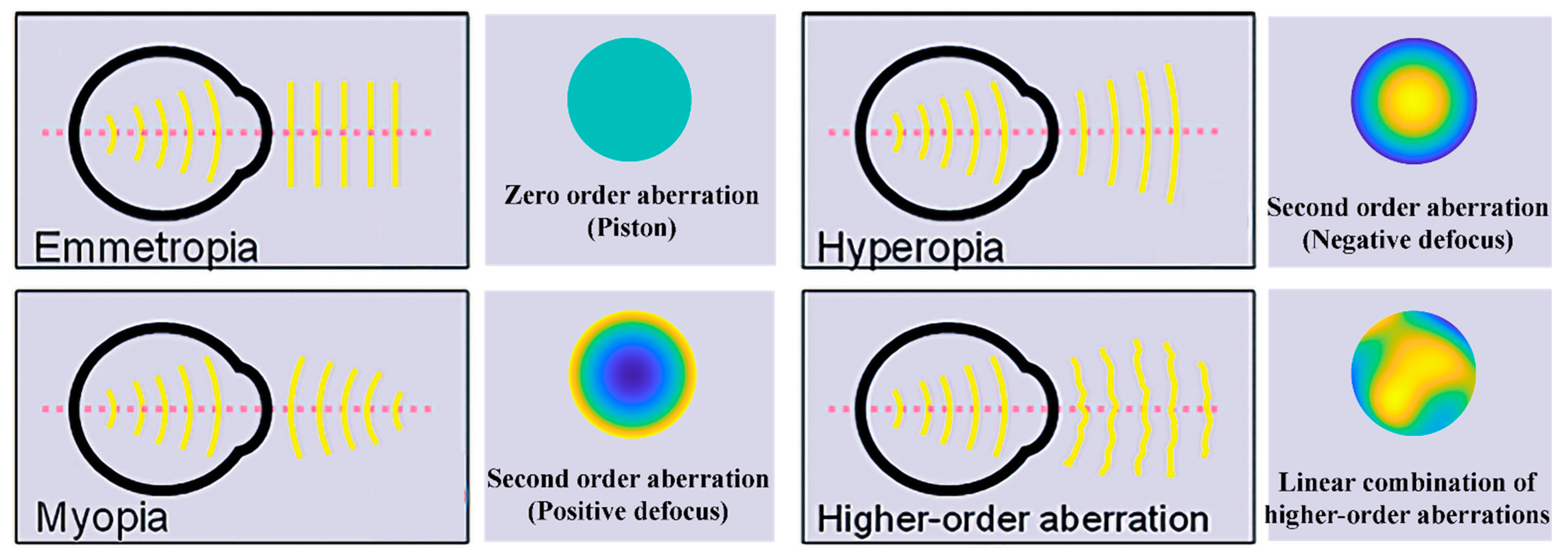
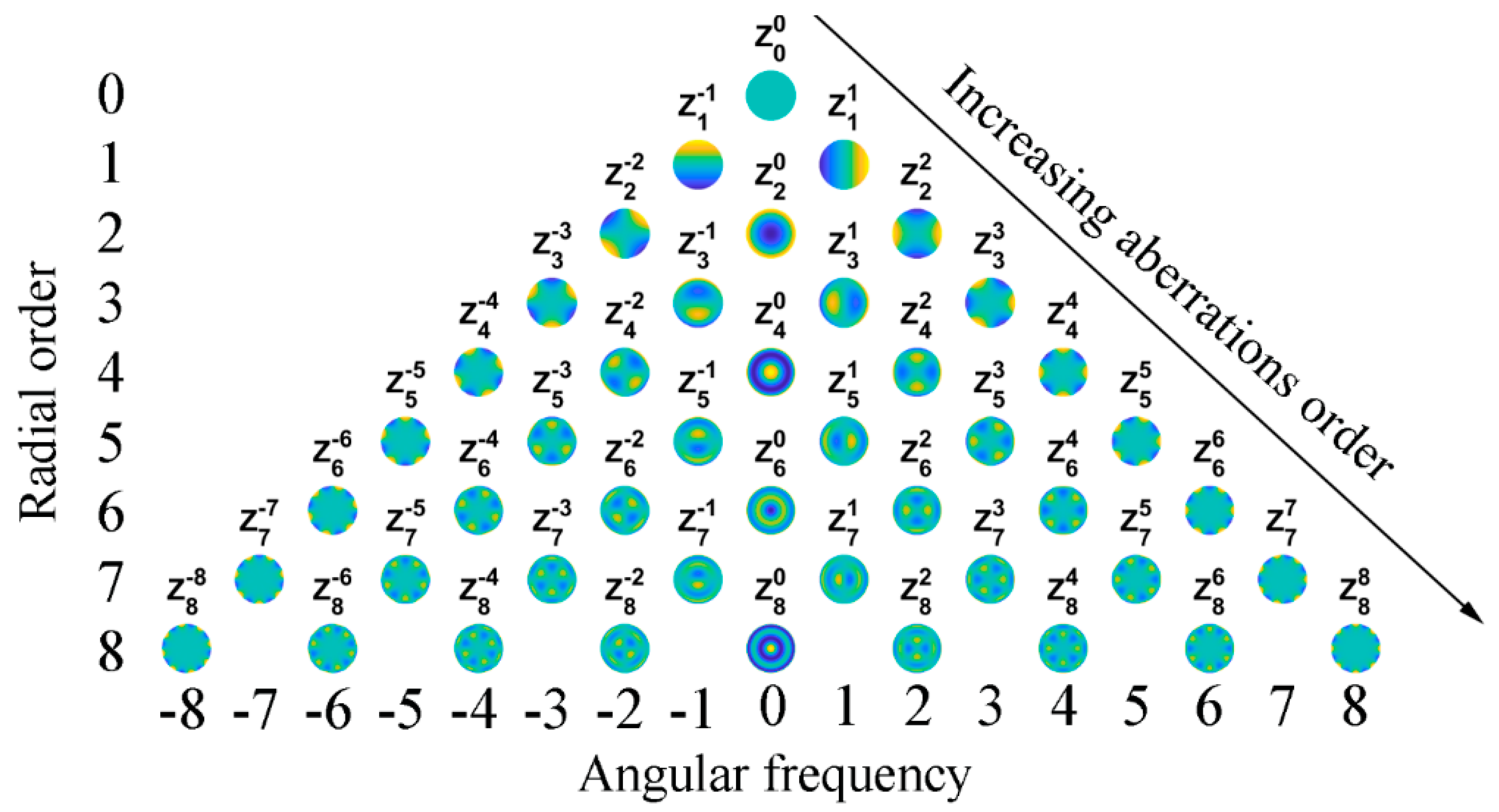
2. Wavefront Analysis Based on Zernike Polynomials
3. Wavefront Sensors for Ophthalmological Applications: Physical Principle and Practice

| Description | Advantage | Drawback | |
|---|---|---|---|
| Shack–Hartmann WS | Detection of spot displacements thanks to a lenslet array and a reference grid. | Flexibility and adaptability to different measurement systems [24]. | Limited dynamic range [15] and limited spatial sampling [25]. Not suitable for high-resolution phase measurement [26]. Cost [24]. |
| Pyramid Sensor | A pyramid prism divides the incoming light into four different spots on a CCD surface. Their differences provide information about WF gradients. | Adjustable sampling and dynamic range [27]. | Spurious reflections, necessity of another device for modulation [27]. |
| Curvature Sensor | Two detectors are symmetrically placed with respect to the focal plane. Their difference in intensity provides information about the second derivative of the WF. | Compared to S–H, higher dynamic range and lower cost [15]. | Long measurement time and less accurate for higher-order aberrations [15]. |
| Optical Differentiation WS | A system of lenses and a mask is used to obtain WF phase slope thanks to Fourier transform properties. | Achromaticity, high resolution, and large dynamic range [28]. | Lost absorbed energy [29]. Compared to S–H, worse signal-to-noise ratio [29]. |
| Diffuser WS | A thin diffuser is set close to the detector and its memory effect is used to retrieve WF displacements. | Low cost, large dynamic range [24]. | Slow computational time [30]. |
| Shearing Interferometry | The interference pattern between the incoming wavefront and its displaced replica is used to measure the wavefront phase. | No need for a reference wave [15] | Limited dynamicrange [31]. |
| Tscherning Aberrometer | A collimated laser beam illuminates a mask with regular matrix pin holes, forming a bundle of thin parallel rays. The deviations of all spots from their ideal regular positions are associated with the optical aberrations, computed in the form of Zernike polynomials up to the 8th order. | Fast measuring and highly accurate. | Not patient friendly because it requires more time and effort to obtain treatable image [32]. |
| Dynamic Range | Sensitivity | |
|---|---|---|
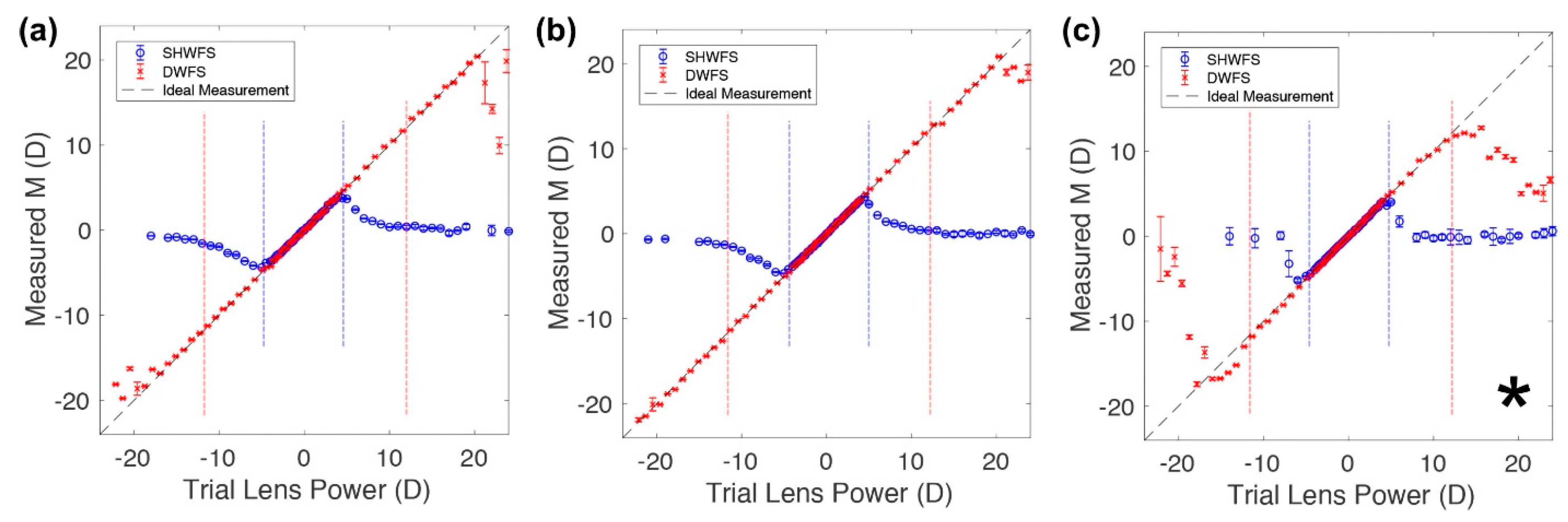
| Shack–Hartmann WS | −4 D to 4.5 D [24] | 0.13 D [24] |
| Pyramid Sensor | − [15] | + [33] |
| Curvature Sensor | + [15] | − [15] |
| Optical Differentiation WS | + [28] | − [28] |
| Diffuser WS | + [24] | + [24] |
| Multiple Shearing Interferometry | + [34] | + [34] |
| Talbot Moiré Interferometry | + [35] | Not available |
| Tscherning Aberrometer | + [36] | Not available |
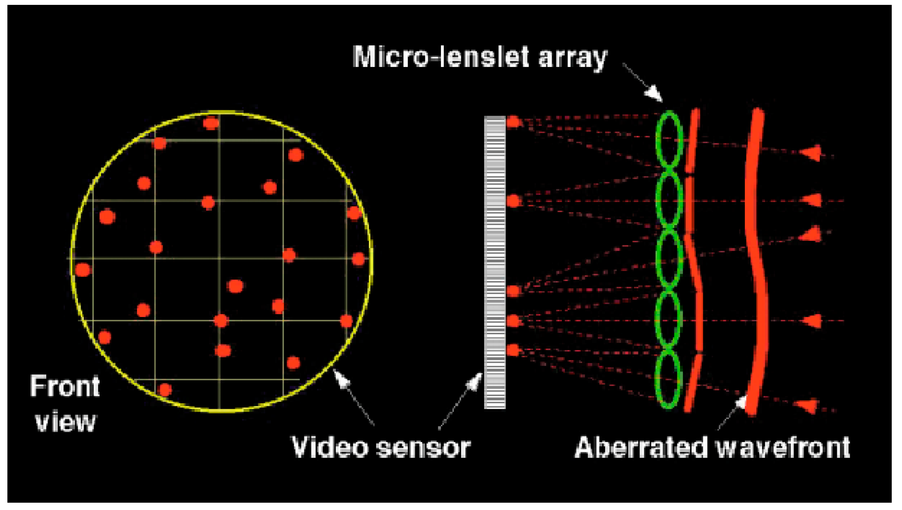
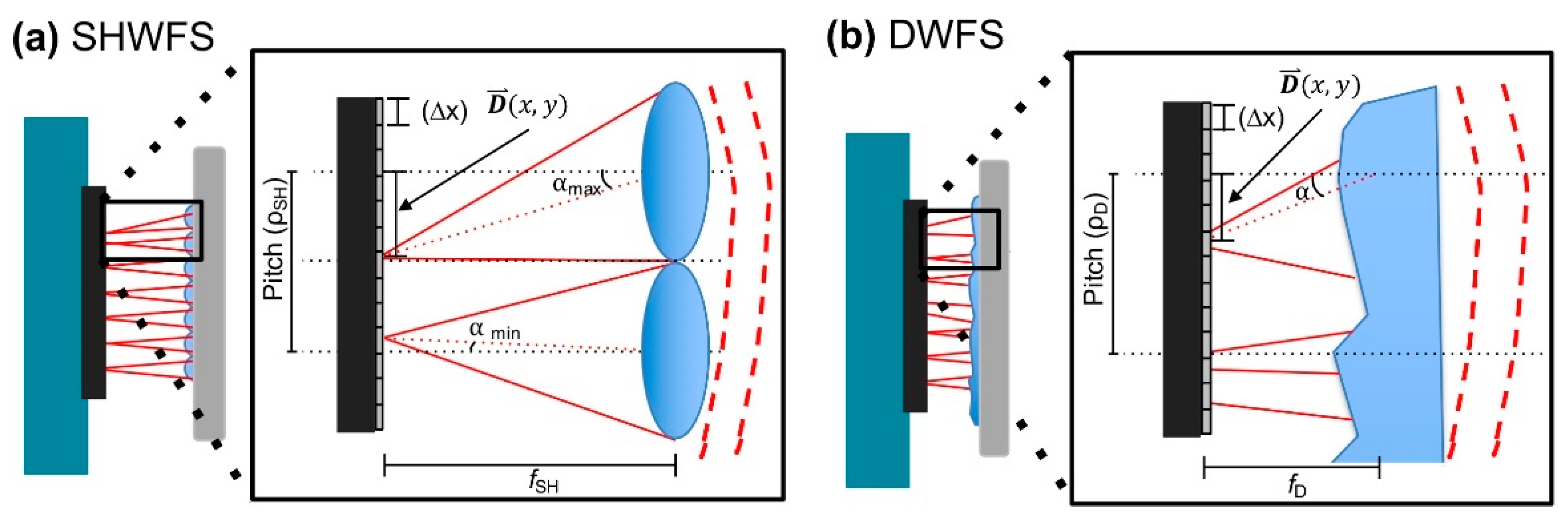
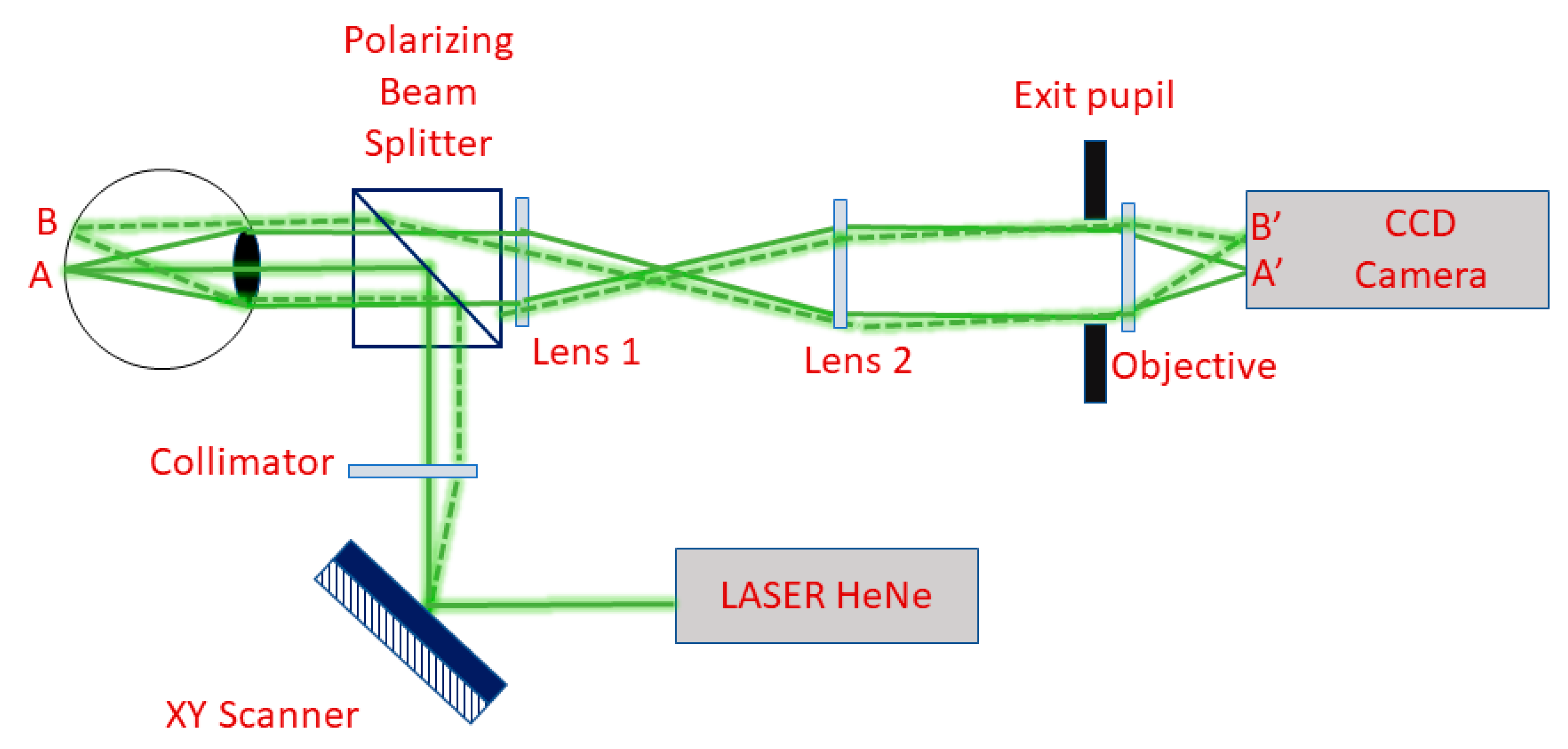
3.1. Shack–Hartmann Sensor
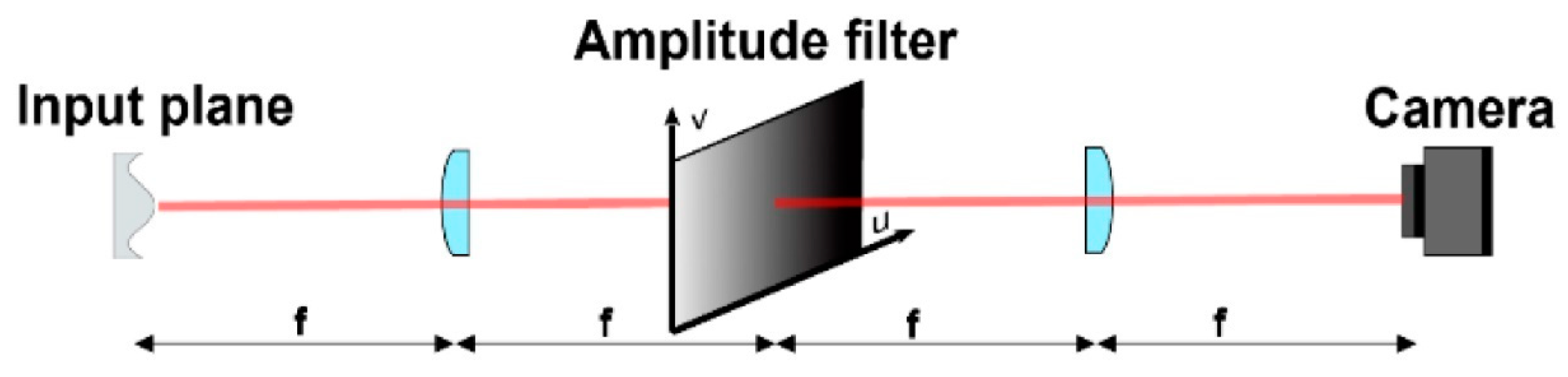
3.2. Foucault Knife-Edge and Optical Differentiation Wavefront Sensor (ODWS)
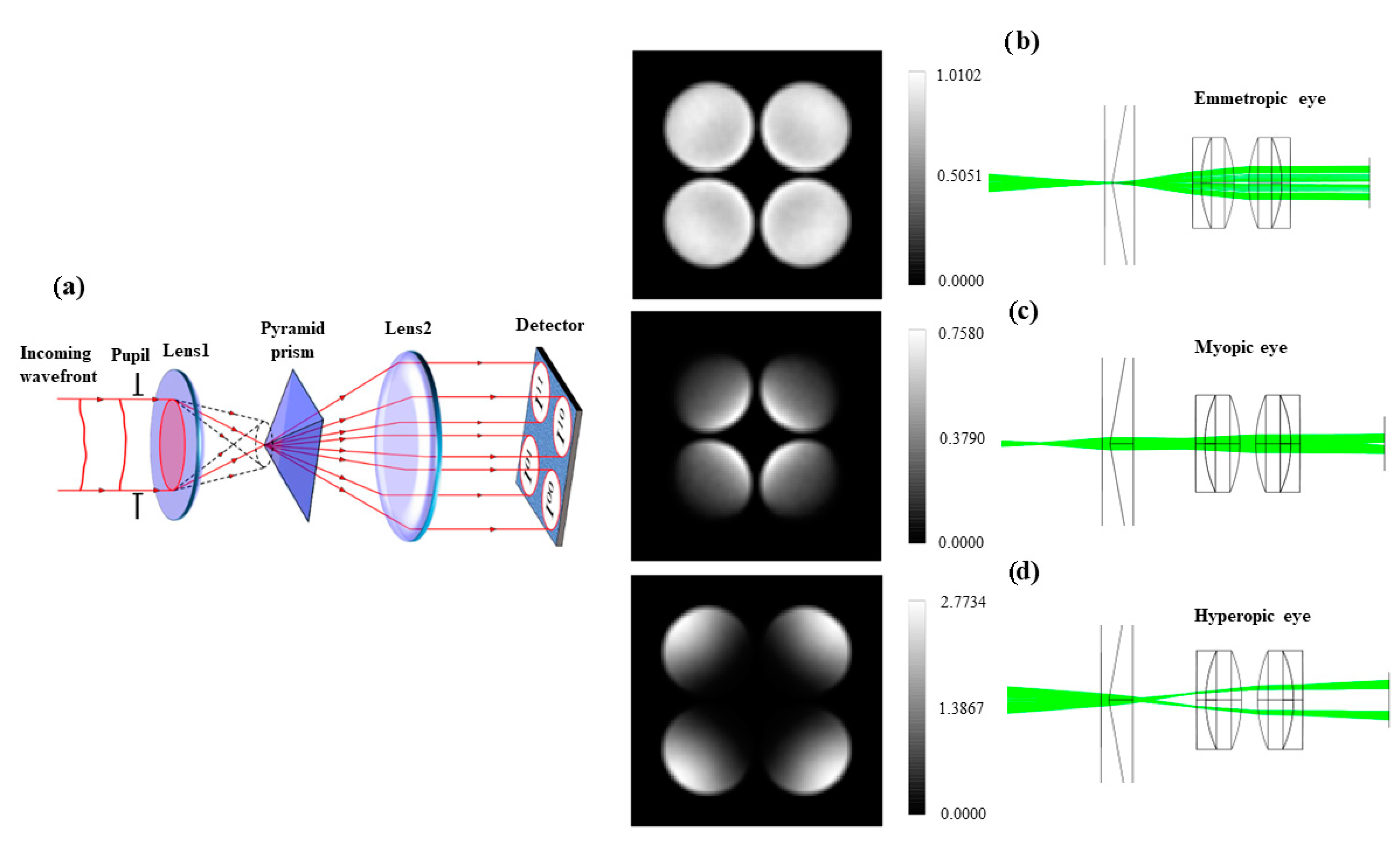
3.3. Pyramid Sensor
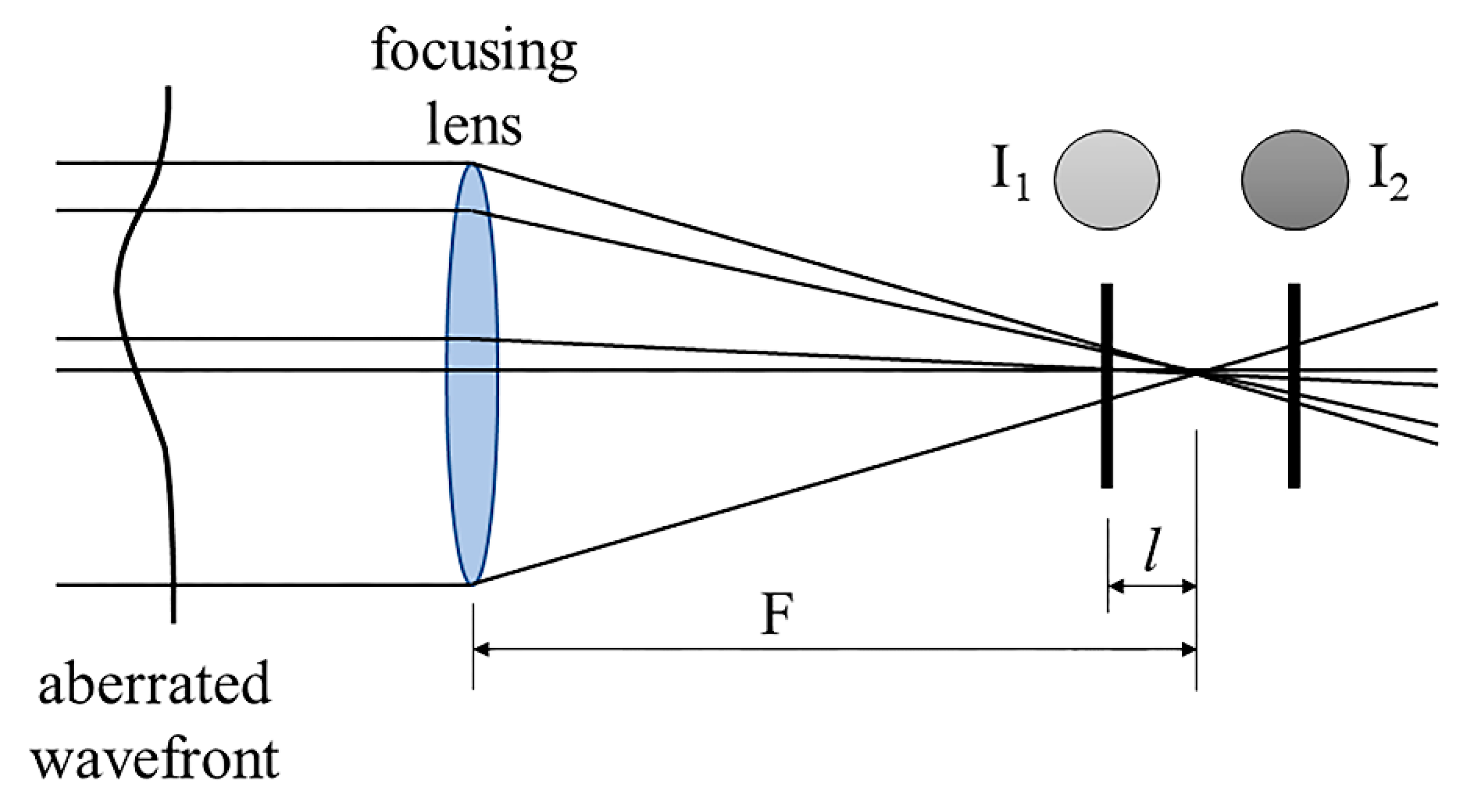
3.4. Curvature and Phase Diversity Wavefront Sensors
3.5. Diffuser Wavefront Sensor
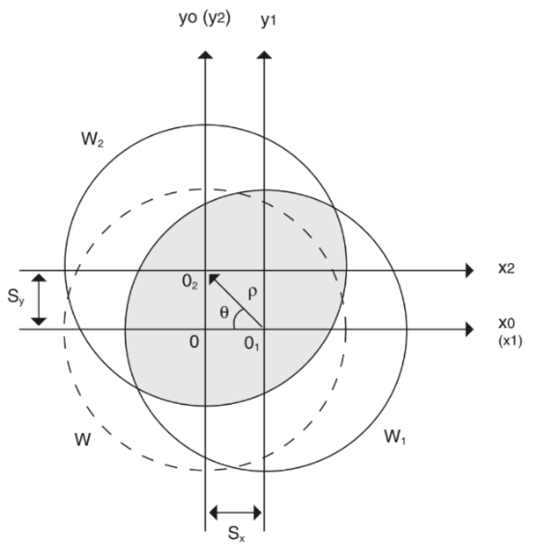
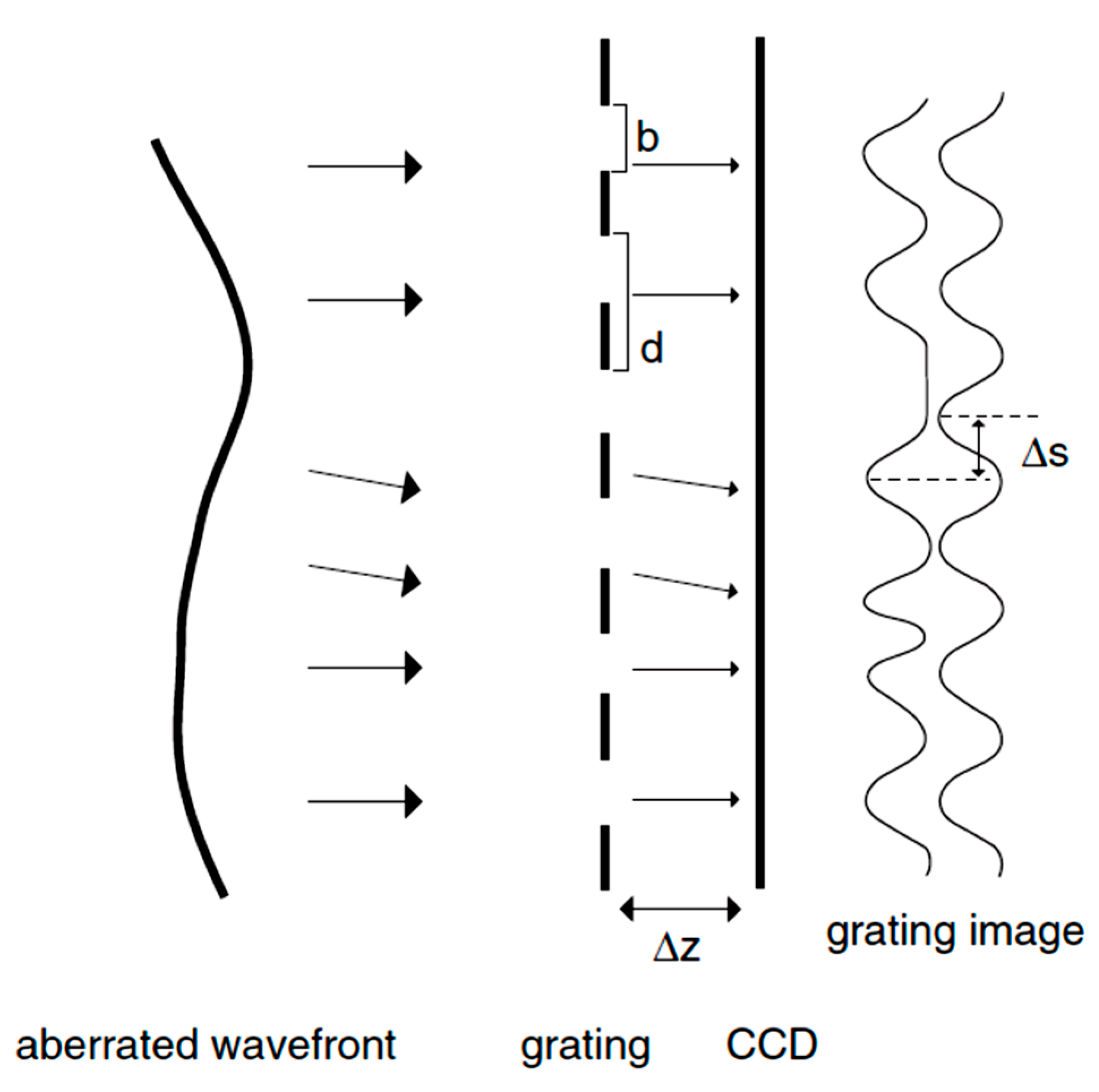
3.6. Shearing Interferometry
Talbot Moiré Technology
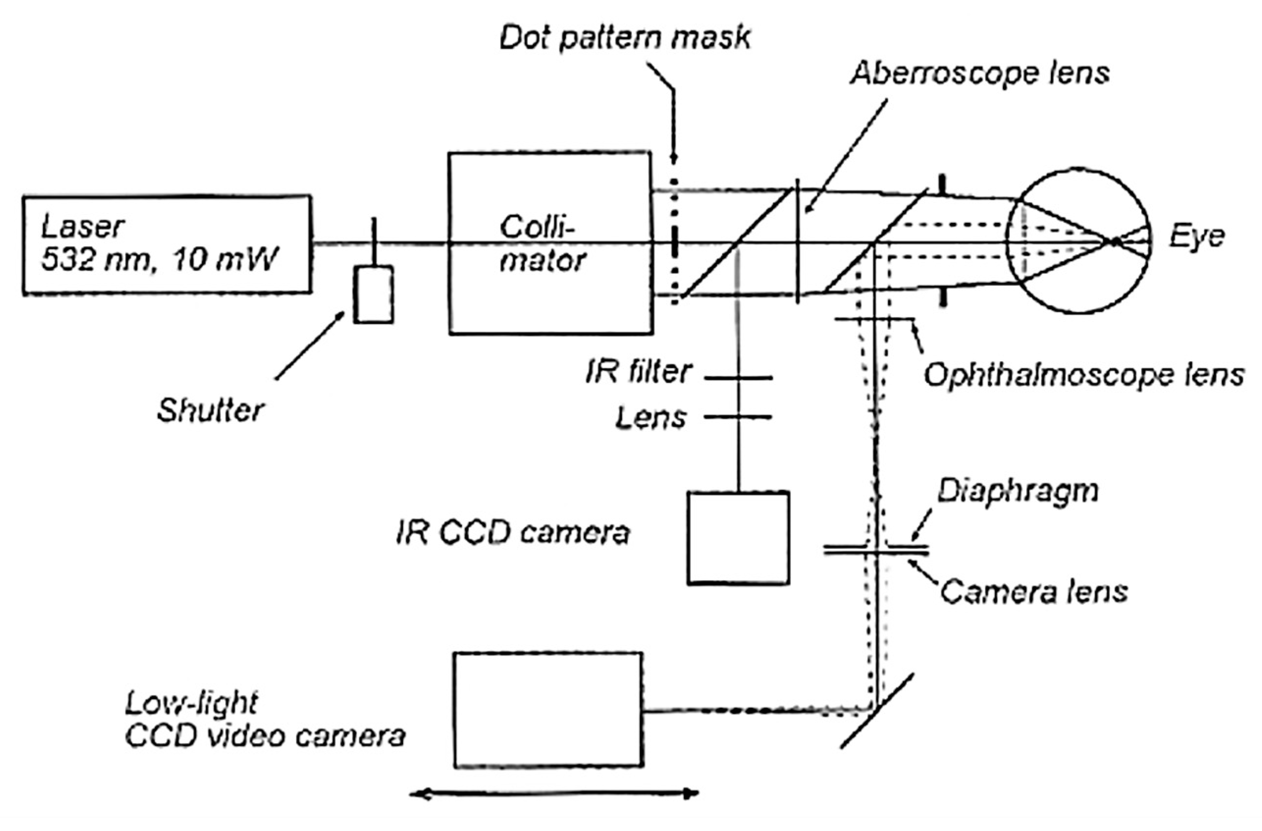
3.7. Tscherning Aberrometer, Ray-Tracing System, and Dynamic Skiascopy
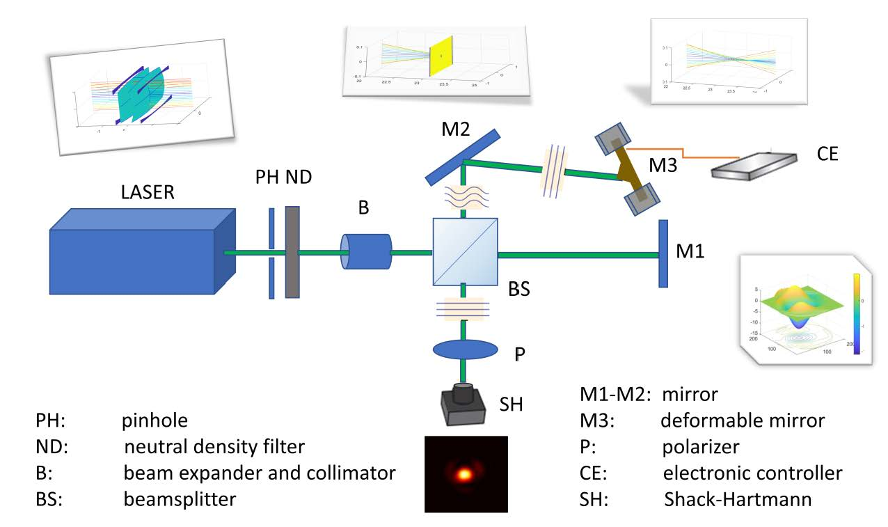
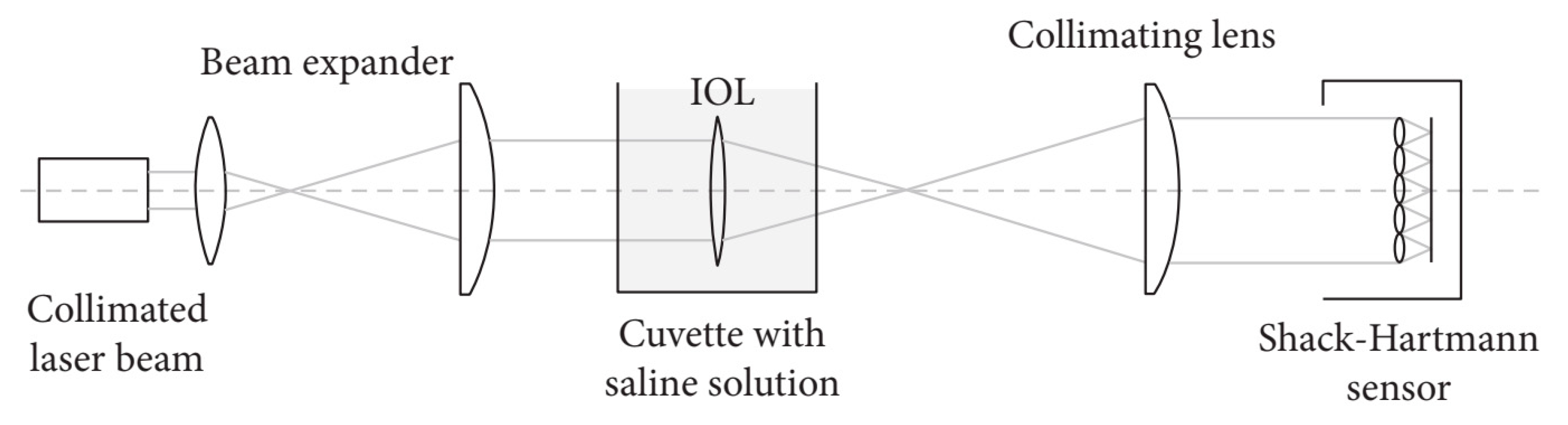
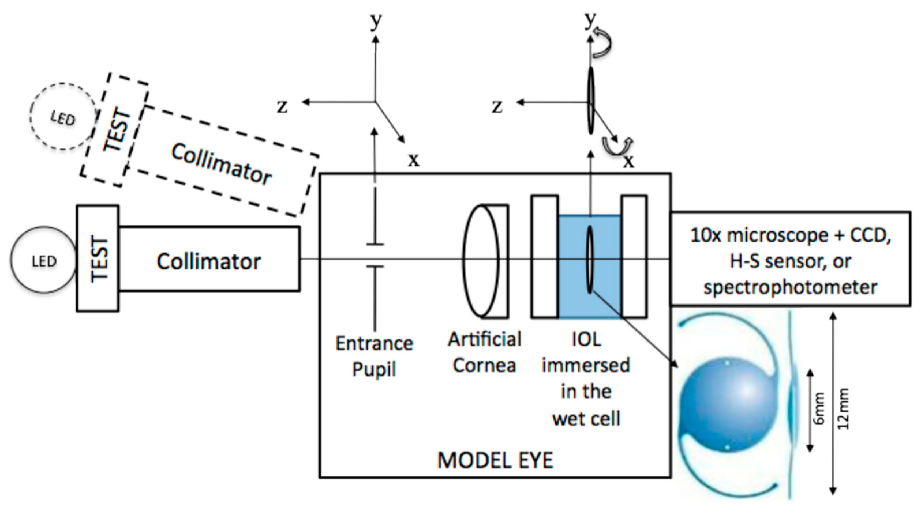
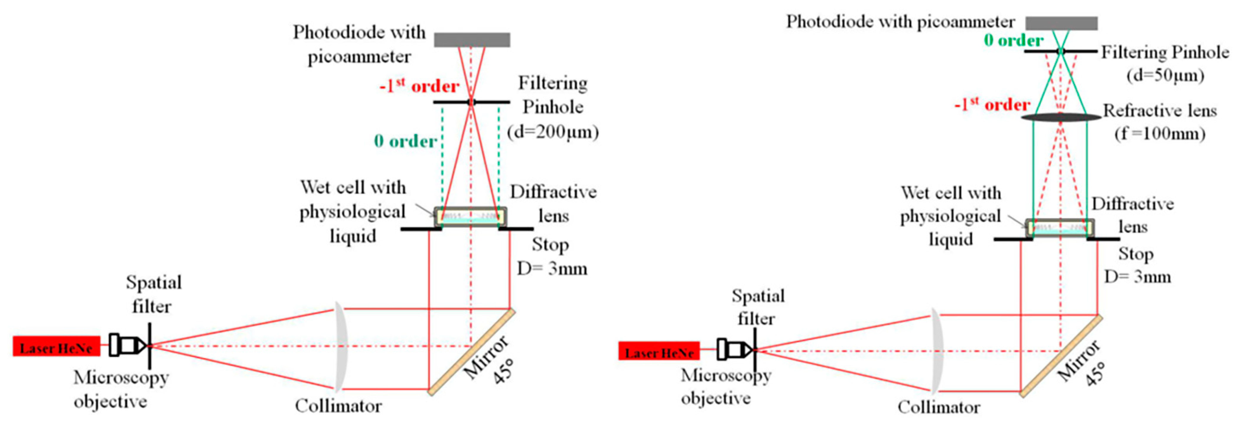
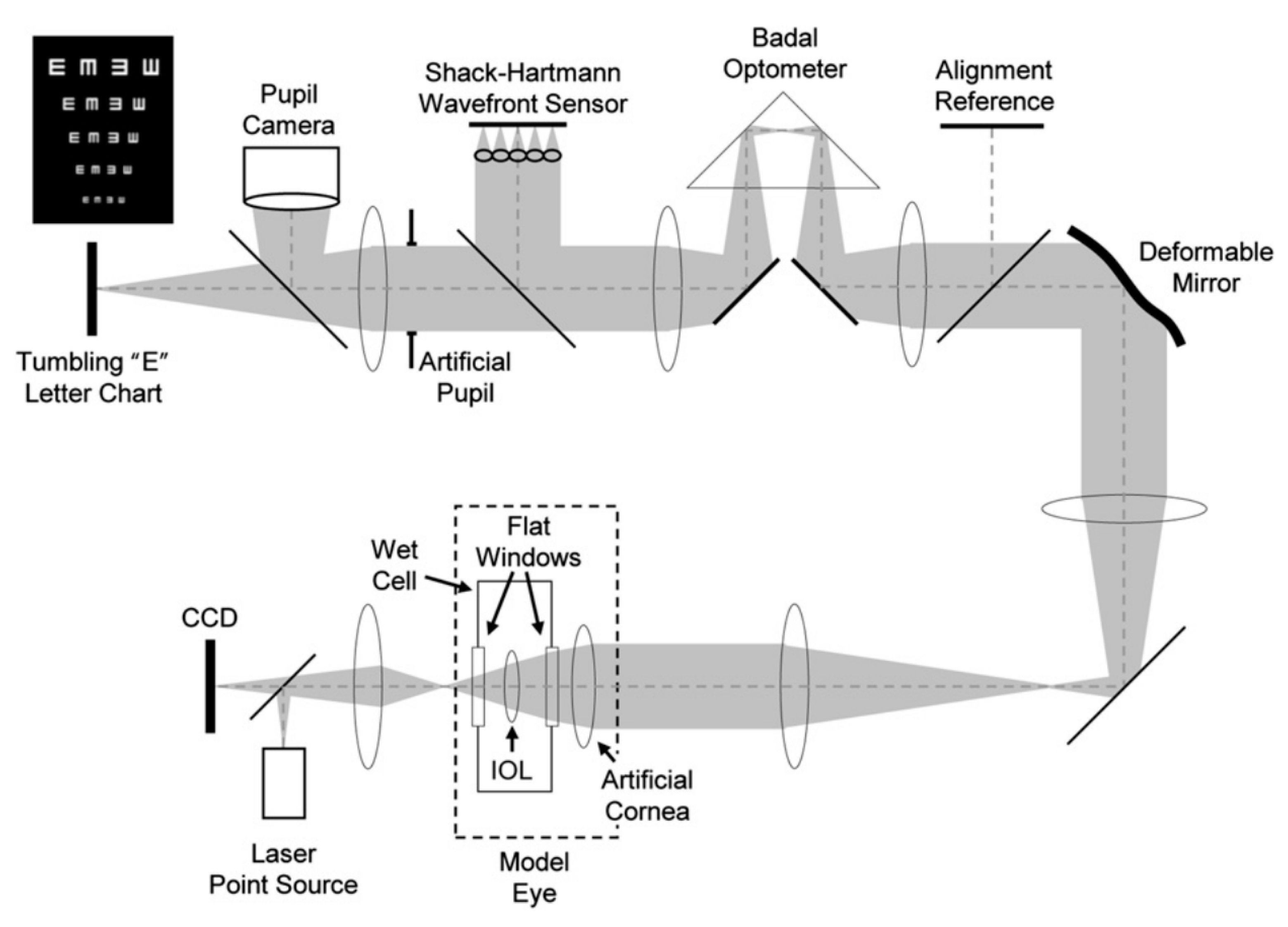
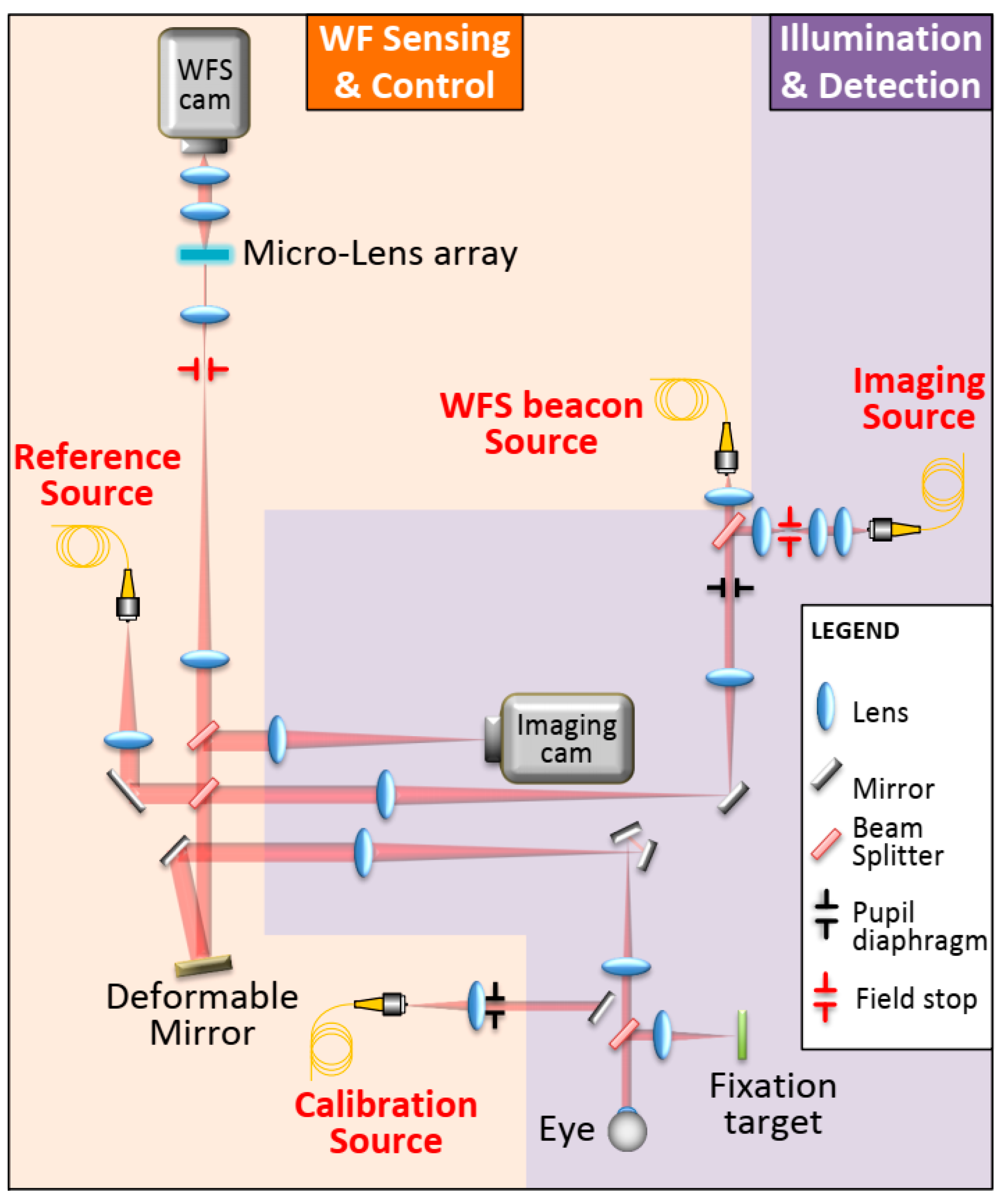
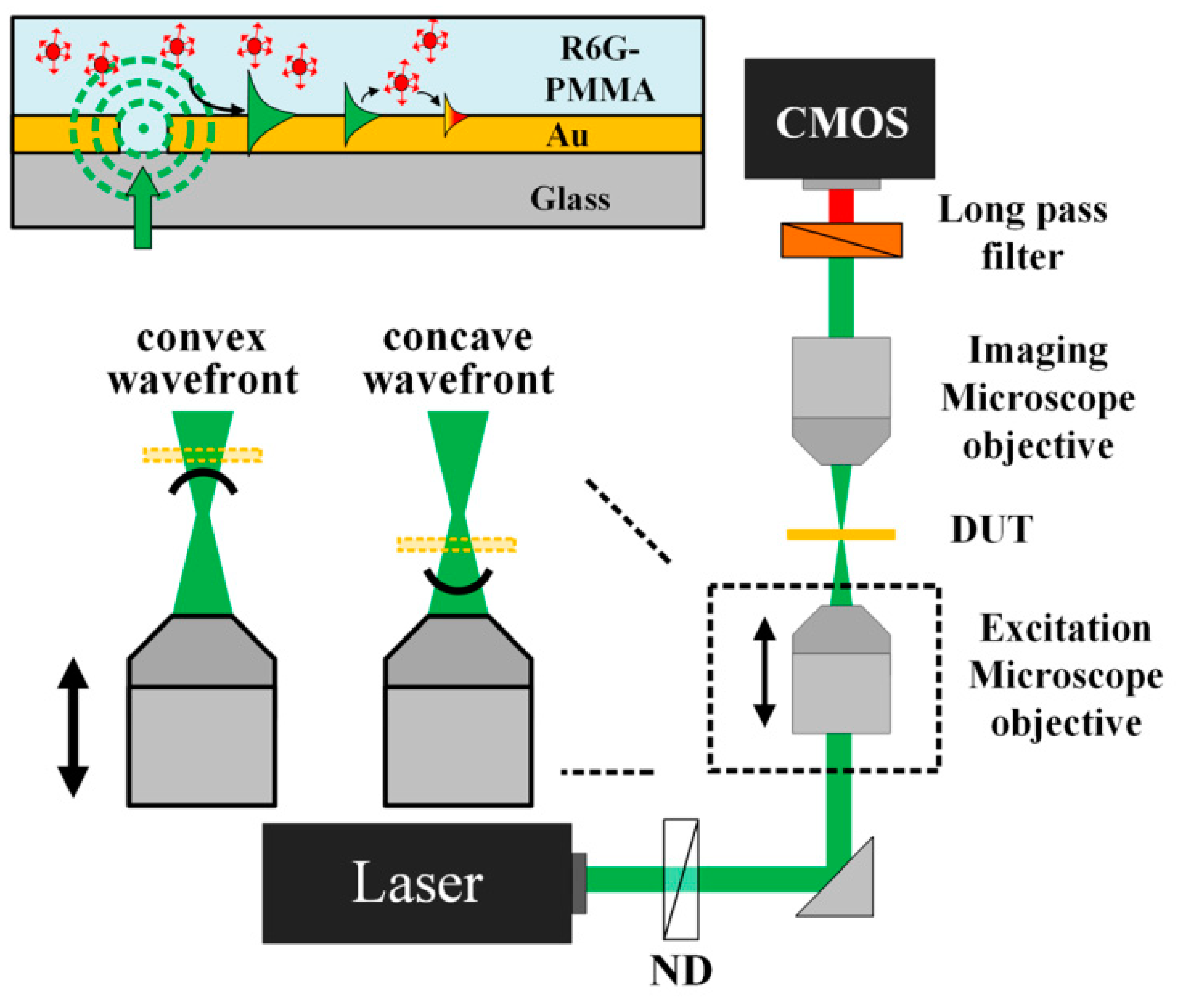
4. IOLs Wavefront Aberrations Experimental Setups
5. Applications
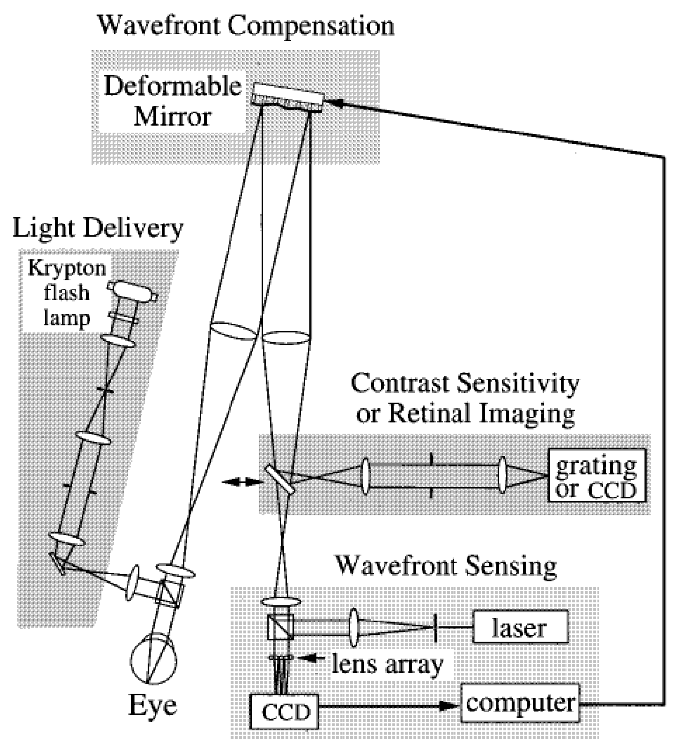
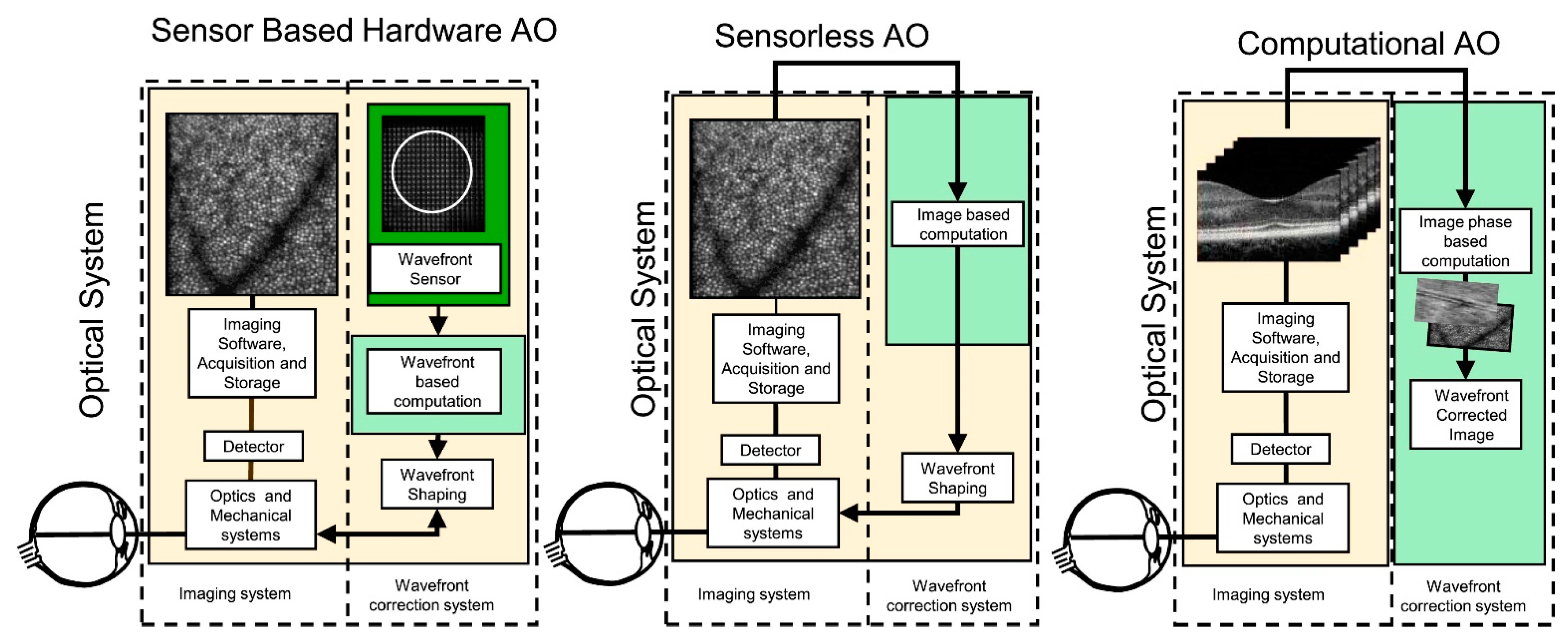
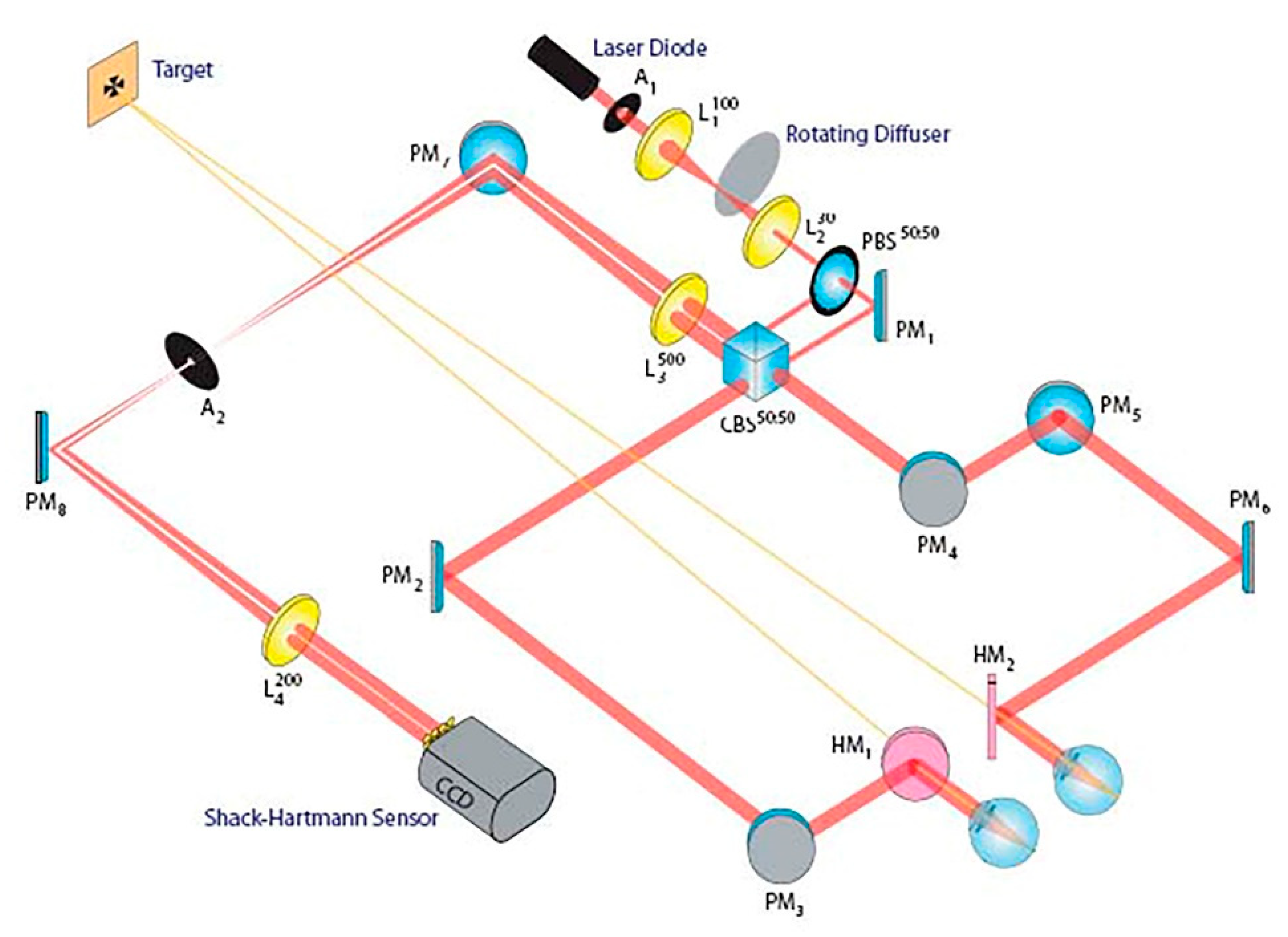
5.1. Adaptive Optics
5.2. Clinical Applications of Intraocular Lens Design
5.2.1. Intraocular Lens Design for Wavefront-Shaping Extended Range-of-Vision
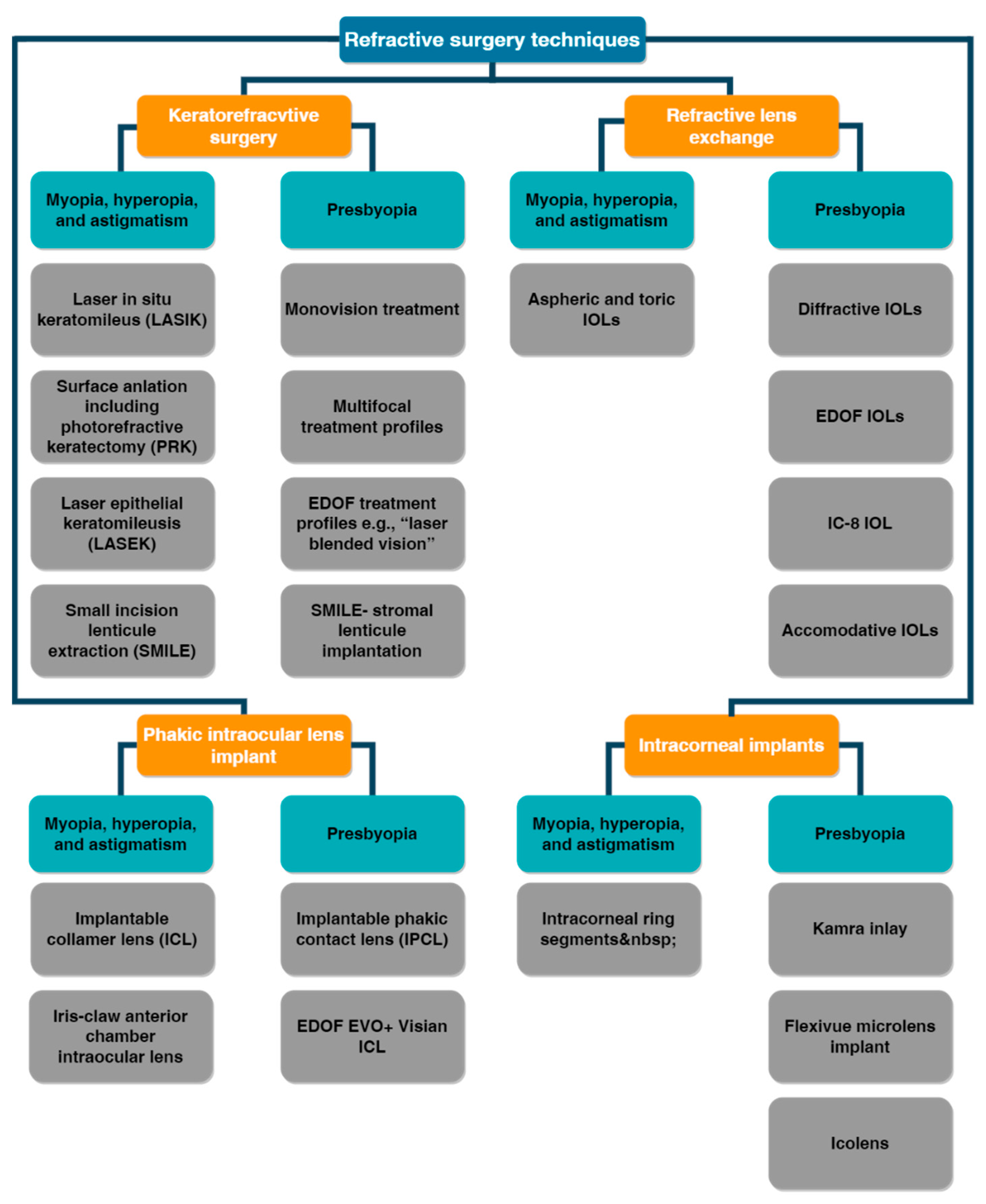
5.2.2. Refractive Surgery
5.2.3. WFS Combined with Ophthalmic Technologies
6. Wavefront Sensing Technology to Empower Clinical Ophthalmic Surgery Application of Multifocal IOLs: Future Developments
7. Conclusions
Author Contributions
Funding
Institutional Review Board Statement
Data Availability Statement
Conflicts of Interest
References
- Kugler, L.J.; Wang, M.X. Lasers in Refractive Surgery: History, Present, and Future. Appl. Opt. 2010, 49, F1. [Google Scholar] [CrossRef] [PubMed] [Green Version]
- Kligman, B.E.; Baartman, B.J.; Dupps, W.J. Errors in Treatment of Lower-Order Aberrations and Induction of Higher-Order Aberrations in Laser Refractive Surgery. Int. Ophthalmol. Clin. 2016, 56, 19–45. [Google Scholar] [CrossRef] [Green Version]
- Maeda, N. Clinical Applications of Wavefront Aberrometry—A Review. Clin. Exp. Ophthalmol. 2009, 37, 118–129. [Google Scholar] [CrossRef]
- Charman, W.N. Wavefront Technology: Past, Present and Future. Contactlens Anterior Eye 2005, 28, 75–92. [Google Scholar] [CrossRef] [PubMed]
- Briguglio, R.A.; Agapito, G.; del Vecchio, C.; Pinna, E.; Xompero, M.; Arcidiacono, C.; Terreri, A.; Pedichini, F. Demonstrating the Sub-Nanometer Sensitivity of a Pyramid WaveFrontSensor for Active Space Telescopes. In Proceedings of the International Conference on Space Optics—ICSO 2020; Sodnik, Z., Cugny, B., Karafolas, N., Eds.; SPIE: Bellingham, WA, USA, 2021; p. 1185251. [Google Scholar]
- Perrin, M.D.; Acton, D.S.; Lajoie, C.-P.; Knight, J.S.; Lallo, M.D.; Allen, M.; Baggett, W.; Barker, E.; Comeau, T.; Coppock, E.; et al. Preparing for JWST Wavefront Sensing and Control Operations. In Proc. SPIE 9904, Space Telescopes and Instrumentation 2016: Optical, Infrared, and Millimeter Wave; MacEwen, H.A., Fazio, G.G., Lystrup, M., Batalha, N., Siegler, N., Tong, E.C., Eds.; SPIE: Bellingham, WA, USA, 2016; p. 99040F. [Google Scholar]
- Maeda, N. Wavefront Technology in Ophthalmology. Curr. Opin. Ophthalmol. 2001, 12, 294–299. [Google Scholar] [CrossRef] [PubMed]
- Ryan, D.S.; Sia, R.K.; Rabin, J.; Rivers, B.A.; Stutzman, R.D.; Pasternak, J.F.; Eaddy, J.B.; Logan, L.A.; Bower, K.S. Contrast Sensitivity After Wavefront-Guided and Wavefront-Optimized PRK and LASIK for Myopia and Myopic Astigmatism. J. Refract. Surg. 2018, 34, 590–596. [Google Scholar] [CrossRef] [PubMed]
- Piñero, D.P.; Soto-Negro, R.; Ruiz-Fortes, P.; Pérez-Cambrodí, R.J.; Fukumitsu, H. Analysis of Intrasession Repeatability of Ocular Aberrometric Measurements and Validation of Keratometry Provided by a New Integrated System in Mild to Moderate Keratoconus. Cornea 2019, 38, 1097–1104. [Google Scholar] [CrossRef]
- Hampson, K.M. Adaptive Optics and Vision. J. Mod. Opt. 2008, 55, 3425–3467. [Google Scholar] [CrossRef]
- Yoon, G. Wavefront Sensing and Diagnostic Uses. In Adaptive Optics for Vision Science; John Wiley & Sons, Inc.: Hoboken, NJ, USA, 2005; pp. 63–81. [Google Scholar]
- Bille, J.F.; Harner, C.F.; Lösel, F. Aberration-Free Refractive Surgery: New Frontiers in Vision; Bille, J.F., Harner, C.F.H., Loesel, F.F., Eds.; Springer: Berlin/Heidelberg, Germany, 2004; ISBN 978-3-642-62111-6. [Google Scholar]
- Lakshminarayanan, V.; Fleck, A. Zernike Polynomials: A Guide. J. Mod. Opt. 2011, 58, 545–561. [Google Scholar] [CrossRef]
- Applegate, R.A. Glenn Fry Award Lecture 2002: Wavefront Sensing, Ideal Corrections, and Visual Performance. Optom. Vis. Sci. 2004, 81, 167–177. [Google Scholar] [CrossRef] [PubMed]
- Lombardo, M.; Lombardo, G. New Methods and Techniques for Sensing the Wave Aberrations of Human Eyes. Clin. Exp. Optom. 2009, 92, 176–186. [Google Scholar] [CrossRef] [PubMed]
- He, J.C.; Burns, S.A.; Marcos, S. Monochromatic Aberrations in the Accommodated Human Eye. Vis. Res. 2000, 40, 41–48. [Google Scholar] [CrossRef] [PubMed]
- Chen, L.; Singer, B.; Guirao, A.; Porter, J.; Williams, D.R. Image Metrics for Predicting Subjective Image Quality. Optom. Vis. Sci. 2005, 82, 358–369. [Google Scholar] [CrossRef] [PubMed] [Green Version]
- Harvey, J.E.; Ftaclas, C. Diffraction Effects of Telescope Secondary Mirror Spiders on Various Image-Quality Criteria. Appl. Opt. 1995, 34, 6337–6349. [Google Scholar] [CrossRef] [PubMed]
- Ottevaere, H.; Thienpont, H. Optical microlenses. In Encyclopedia of Modern Optics; Elsevier: Amsterdam, The Netherlands, 2005; pp. 21–43. [Google Scholar]
- Lawless, M.A.; Hodge, C. Wavefront’s Role in Corneal Refractive Surgery. Clin. Exp. Ophthalmol. 2005, 33, 199–209. [Google Scholar] [CrossRef]
- Wang, K.; Xu, K. A Review on Wavefront Reconstruction Methods. In Proceedings of the 2021 4th International Conference on Information Systems and Computer Aided Education, Dalian, China, 24–26 September 2021; ACM: New York, NY, USA, 2021; pp. 1528–1531. [Google Scholar]
- Li, Z.; Li, X.; Gao, Z.; Jia, Q. Review of Wavefront Sensing Technology in Adaptive Optics Based on Deep Learning. High Power Laser Part. Beams 2021, 33, 081001. [Google Scholar] [CrossRef]
- Mello, G.R.; Rocha, K.M.; Santhiago, M.R.; Smadja, D.; Krueger, R.R. Applications of Wavefront Technology. J. Cataract Refract. Surg. 2012, 38, 1671–1683. [Google Scholar] [CrossRef]
- McKay, G.N.; Mahmood, F.; Durr, N.J. Large Dynamic Range Autorefraction with a Low-Cost Diffuser Wavefront Sensor. Biomed. Opt. Express 2019, 10, 1718–1735. [Google Scholar] [CrossRef]
- Greivenkamp, J.E.; Smith, D.G.; Gappinger, R.O.; Williby, G.A. Optical Testing Using Shack-Hartmann Wavefront Sensors. In Proceedings of the Optical Engineering for Sensing and Nanotechnology (ICOSN ’01), Yokohama, Japan, 6–8 June 2001; Iwata, K., Ed.; SPIE: Bellingham, WA, USA, 2001; p. 260. [Google Scholar] [CrossRef]
- Haffert, S.Y. Generalised Optical Differentiation Wavefront Sensor: A Sensitive High Dynamic Range Wavefront Sensor. Opt. Express 2016, 24, 18986–19007. [Google Scholar] [CrossRef]
- Iglesias, I.; Ragazzoni, R.; Julien, Y.; Artal, P. Extended Source Pyramid Wave-Front Sensor for the Human Eye. Opt. Express 2002, 10, 419–428. [Google Scholar] [CrossRef]
- Swain, B.R.; Dorrer, C.; Qiao, J. High-Performance Optical Differentiation Wavefront Sensing towards Freeform Metrology. Opt. Express 2019, 27, 36297–36310. [Google Scholar] [CrossRef] [PubMed]
- Oti, J.E.; Canales, V.F.; Cagigal, M.P. Improvements on the Optical Differentiation Wavefront Sensor. Mon. Not. R. Astron. Soc. 2005, 360, 1448–1454. [Google Scholar] [CrossRef] [Green Version]
- Berto, P.; Rigneault, H.; Guillon, M. Wavefront Sensing with a Thin Diffuser. Opt. Lett. 2017, 42, 5117–5120. [Google Scholar] [CrossRef] [PubMed] [Green Version]
- Xue, S.; Chen, S.; Fan, Z.; Zhai, D. Adaptive Wavefront Interferometry for Unknown Free-Form Surfaces. Opt. Express 2018, 26, 21910–21928. [Google Scholar] [CrossRef] [PubMed]
- Mrochen, M.; Kaemmerer, M.; Mierdel, P.; Krinke, H.-E.; Seiler, T. Principles of Tscherning Aberrometry. J. Refract. Surg. 2000, 16, S570–S571. [Google Scholar] [CrossRef]
- Ragazzoni, R.; Farinato, J. Sensitivity of a Pyramidic Wave Front Sensor in Closed Loop Adaptive Optics. Astron. Astrophys. 1999, 350, L23–L26. [Google Scholar]
- Chanteloup, J.-C. Multiple-Wave Lateral Shearing Interferometry for Wave-Front Sensing. Appl. Opt. 2005, 44, 1559–1571. [Google Scholar] [CrossRef]
- Wiley, W.F.; Bafna, S. Intra-Operative Aberrometry Guided Cataract Surgery. Int. Ophthalmol. Clin. 2011, 51, 119–129. [Google Scholar] [CrossRef]
- Solomon, K.D.; Fernandez De Castro, L.E.; Sandoval, H.P.; Vroman, D.T. Comparison of Wavefront Sensing Devices. Ophthalmol. Clin. N. Am. 2004, 17, 119–127. [Google Scholar] [CrossRef]
- Hartmann, J. Bemerkungen Über Den Bau Und Die Justirung von Spektrographen. Zt. Instrum. 1900, 20, 47. [Google Scholar]
- Shack, R.V.; Platt, B.C. Production and Use of a Lenticular Hartmann Screen. J. Opt. Soc. Am. 1971, 61, 656–661. [Google Scholar]
- Rasouli, S.; Dashti, M.; Ramaprakash, A.N. An Adjustable, High Sensitivity, Wide Dynamic Range Two Channel Wave-Front Sensor Based on Moiré Deflectometry. Opt. Express 2010, 18, 23906–23915. [Google Scholar] [CrossRef] [PubMed]
- Platt, B.C.; Shack, R. History and Principles of Shack-Hartmann Wavefront Sensing. J. Refract. Surg. 2001, 17, S573–S577. [Google Scholar] [CrossRef] [PubMed]
- Rousset, G. Wave-Front Sensors. In Adaptive Optics in Astronomy; Roddier, F., Ed.; Cambridge University Press: Cambridge, UK, 1999; pp. 91–130. ISBN 9780521553759. [Google Scholar]
- Shinto, H.; Saita, Y.; Nomura, T. Shack–Hartmann Wavefront Sensor with Large Dynamic Range by Adaptive Spot Search Method. Appl. Opt. 2016, 55, 5413–5418. [Google Scholar] [CrossRef] [PubMed]
- Akondi, V.; Dubra, A. Shack-Hartmann Wavefront Sensor Optical Dynamic Range. Opt. Express 2021, 29, 8417–8429. [Google Scholar] [CrossRef] [PubMed]
- Ehrenfest, P. Notes on the Approximate Validity of Quantum Mechanics. Z. Phys. 1927, 45, 455–457. [Google Scholar] [CrossRef]
- Cook, R.J. Beam Wander in a Turbulent Medium: An Application of Ehrenfest’s Theorem. J. Opt. Soc. Am. 1975, 65, 942–948. [Google Scholar] [CrossRef]
- Bará, S. Characteristic Functions of Hartmann-Shack Wavefront Sensors and Laser-Ray-Tracing Aberrometers. J. Opt. Soc. Am. A 2007, 24, 3700–3707. [Google Scholar] [CrossRef]
- Thibos, L.N. Principles of Hartmann-Shack Aberrometry. In Vision Science and its Applications; OSA: Washington, DC, USA, 2000; p. NW6. [Google Scholar]
- Moreno-Barriuso, E.; Marcos, S.; Navarro, R.; Burns, S.A. Comparing Laser Ray Tracing, the Spatially Resolved Refractometer, and the Hartmann-Shack Sensor to Measure the Ocular Wave Aberration. Optom. Vis. Sci. 2001, 78, 152–156. [Google Scholar] [CrossRef]
- Wu, Y.; Sharma, M.K.; Veeraraghavan, A. WISH: Wavefront Imaging Sensor with High Resolution. Light Sci. Appl. 2019, 8, 44. [Google Scholar] [CrossRef] [Green Version]
- Burvall, A.; Daly, E.; Chamot, S.R.; Dainty, C. Linearity of the Pyramid Wavefront Sensor. Opt. Express 2006, 14, 11925–11934. [Google Scholar] [CrossRef] [PubMed]
- Ojeda-Castaeda, J. Foucault, Wire, and Phase Modulation Tests. In Optical Shop Testing; John Wiley & Sons, Inc.: Hoboken, NJ, USA, 1992; pp. 275–316. [Google Scholar]
- Wang, H.; Liu, C.; He, X.; Pan, X.; Zhou, S.; Wu, R.; Zhu, J. Wavefront Measurement Techniques Used in High Power Lasers. High Power Laser Sci. Eng. 2014, 2, e25. [Google Scholar] [CrossRef]
- Oti, J.; Canales, V.; Cagigal, M. Analysis of the Signal-to-Noise Ratio in the Optical Differentiation Wavefront Sensor. Opt. Express 2003, 11, 2783–2790. [Google Scholar] [CrossRef] [PubMed]
- Oti, J.E.; Canales, V.F.; Cagigal, M.P.; Valle, P.J. Wavefront Sensing by Optical Differentiation. In Proceedings of the 5th International Workshop on Adaptive Optics for Industry and Medicine, Beijing, China, 29 August–1 September 2005; Jiang, W., Ed.; SPIE: Bellingham, WA, USA, 2005; p. 60180P. [Google Scholar]
- Bortz, J.C. Wave-Front Sensing by Optical Phase Differentiation. J. Opt. Soc. Am. A 1984, 1, 35–39. [Google Scholar] [CrossRef]
- Qiao, J.; Mulhollan, Z.; Dorrer, C. Optical Differentiation Wavefront Sensing with Binary Pixelated Transmission Filters. Opt. Express 2016, 24, 9266–9279. [Google Scholar] [CrossRef] [PubMed]
- Sinjab, M.M.; Cummings, A.B. Introduction to Wavefront Science. In Customized Laser Vision Correction; Springer International Publishing: Cham, Switzerland, 2018; pp. 65–93. [Google Scholar]
- Shatokhina, I.; Hutterer, V.; Ramlau, R. Review on Methods for Wavefront Reconstruction from Pyramid Wavefront Sensor Data. J. Astron. Telesc. Instrum. Syst. 2020, 6, 010901. [Google Scholar] [CrossRef]
- Ragazzoni, R. Pupil Plane Wavefront Sensing with an Oscillating Prism. J. Mod. Opt. 1996, 43, 289–293. [Google Scholar] [CrossRef]
- Costa, J.B.; Ragazzoni, R.; Ghedina, A.; Carbillet, M.; Verinaud, C.; Feldt, M.; Esposito, S.; Puga, E.; Farinato, J. Is There Need of Any Modulation in the Pyramid Wavefront Sensor? In Proceedings of SPIE Volume 4839, Adaptive Optical System Technologies II; Wizinowich, P.L., Bonaccini, D., Eds.; SPIE: Bellingham, WA, USA, 2003; p. 288. [Google Scholar]
- Díaz-Doutón, F.; Pujol, J.; Arjona, M.; Luque, S.O. Curvature Sensor for Ocular Wavefront Measurement. Opt. Lett. 2006, 31, 2245–2247. [Google Scholar] [CrossRef]
- Torti, C.; Gruppetta, S.; Diaz-santana, L. Wavefront Curvature Sensing for the Human Eye. J. Mod. Opt. 2008, 55, 691–702. [Google Scholar] [CrossRef] [Green Version]
- Fienup, J.R.; Thelen, B.J.; Paxman, R.G.; Carrara, D.A. Comparison of Phase Diversity and Curvature Wavefront Sensing. In Proceedings of SPIE Volume 3353, Adaptive Optical System Technologies; Bonaccini, D., Tyson, R.K., Eds.; SPIE: Bellingham, WA, USA, 1998; pp. 930–940. [Google Scholar]
- Lombaert, H.; Grady, L.; Pennec, X.; Ayache, N.; Cheriet, F. Spectral Log-Demons: Diffeomorphic Image Registration with Very Large Deformations. Int. J. Comput. Vis. 2014, 107, 254–271. [Google Scholar] [CrossRef] [Green Version]
- Gunjala, G.; Sherwin, S.; Shanker, A.; Waller, L. Aberration Recovery by Imaging a Weak Diffuser. Opt. Express 2018, 26, 21054–21068. [Google Scholar] [CrossRef]
- Baik, S.-H.; Park, S.-K.; Kim, C.-J.; Cha, B. A Center Detection Algorithm for Shack–Hartmann Wavefront Sensor. Opt. Laser Technol. 2007, 39, 262–267. [Google Scholar] [CrossRef]
- Shirai, T.; Barnes, T.H.; Haskell, T.G. Adaptive Wave-Front Correction by Means of All-Optical Feedback Interferometry. Opt. Lett. 2000, 25, 773–775. [Google Scholar] [CrossRef] [PubMed]
- Primot, J. Three-Wave Lateral Shearing Interferometer. Appl. Opt. 1993, 32, 6242–6249. [Google Scholar] [CrossRef] [PubMed]
- Sekine, R.; Shibuya, T.; Ukai, K.; Komatsu, S.; Hattori, M.; Mihashi, T.; Nakazawa, N.; Hirohara, Y. Measurement of Wavefront Aberration of Human Eye Using Talbot Image of Two-Dimensional Grating. Opt. Rev. 2006, 13, 207–211. [Google Scholar] [CrossRef]
- Kim, M.-S.; Scharf, T.; Menzel, C.; Rockstuhl, C.; Herzig, H.P. Talbot Images of Wavelength-Scale Amplitude Gratings. Opt. Express 2012, 20, 4903–4920. [Google Scholar] [CrossRef]
- Lombardo, M.; Serrao, S.; Devaney, N.; Parravano, M.; Lombardo, G. Adaptive Optics Technology for High-Resolution Retinal Imaging. Sensors 2012, 13, 334–366. [Google Scholar] [CrossRef] [Green Version]
- Salama, N.H.; Patrignani, D.; de Pasquale, L.; Sicre, E.E. Wavefront Sensor Using the Talbot Effect. Opt. Laser Technol. 1999, 31, 269–272. [Google Scholar] [CrossRef]
- van Heugten, A. Ophthalmic Talbot-Moire Wavefront Sensor. U.S. Patent US6,736,510 B1, 18 May 2004. [Google Scholar]
- Moreno-Barriuso, E.; Lloves, J.M.; Marcos, S.; Navarro, R.; Llorente, L.; Barbero, S. Ocular Aberrations before and after Myopic Corneal Refractive Surgery: LASIK-Induced Changes Measured with Laser Ray Tracing. Investig. Ophthalmol. Vis. Sci. 2001, 42, 1396–1403. [Google Scholar]
- Tan, B.; Chen, Y.-L.; Baker, K.; Lewis, J.W.; Swartz, T.; Jiang, Y.; Wang, M. Simulation of Realistic Retinoscopic Measurement. Opt. Express 2007, 15, 2753–2761. [Google Scholar] [CrossRef] [PubMed]
- Camps, V.J.; Tolosa, A.; Piñero, D.P.; de Fez, D.; Caballero, M.T.; Miret, J.J. In Vitro Aberrometric Assessment of a Multifocal Intraocular Lens and Two Extended Depth of Focus IOLs. J. Ophthalmol. 2017, 2017, 7095734. [Google Scholar] [CrossRef] [PubMed] [Green Version]
- Alba-Bueno, F.; Vega, F.; Millán, M.S. Design of a Test Bench for Intraocular Lens Optical Characterization. J. Phys. Conf. Ser. 2011, 274, 012105. [Google Scholar] [CrossRef]
- ISO 11979-2:2014; Ophthalmic Implants—Intraocular Lenses—Part 2: Optical Properties and Test Methods. International Organization for Standardization: Geneva, Switzerland, 2014. Available online: https://www.iso.org/standard/55682.html (accessed on 30 November 2022).
- Son, H.S.; Labuz, G.; Khoramnia, R.; Merz, P.; Yildirim, T.M.; Auffarth, G.U. Ray Propagation Imaging and Optical Quality Evaluation of Different Intraocular Lens Models. PLoS ONE 2020, 15, e0228342. [Google Scholar] [CrossRef] [PubMed]
- Vega, F.; Alba-Bueno, F.; Millán, M.S. Energy Distribution between Distance and Near Images in Apodized Diffractive Multifocal Intraocular Lenses. Investig. Ophthalmol. Vis. Sci. 2011, 52, 5695–5701. [Google Scholar] [CrossRef] [PubMed] [Green Version]
- Cohen, A.L. Diffractive Bifocal Lens Designs. Optom. Vis. Sci. 1993, 70, 461–468. [Google Scholar] [CrossRef]
- Tankam, P.; Lépine, T.; Castignoles, F.; Chavel, P. Optical Metrology for Immersed Diffractive Multifocal Ophthalmic Intracorneal Lenses. J. Eur. Opt. Soc. Rapid Publ. 2012, 7, 12037. [Google Scholar] [CrossRef] [Green Version]
- Zheleznyak, L.; Kim, M.J.; MacRae, S.; Yoon, G. Impact of Corneal Aberrations on Through-Focus Image Quality of Presbyopia-Correcting Intraocular Lenses Using an Adaptive Optics Bench System. J. Cataract Refract. Surg. 2012, 38, 1724–1733. [Google Scholar] [CrossRef]
- Luo, C.; Wang, H.; Chen, X.; Xu, J.; Yin, H.; Yao, K. Recent Advances of Intraocular Lens Materials and Surface Modification in Cataract Surgery. Front. Bioeng. Biotechnol. 2022, 10, 913383. [Google Scholar] [CrossRef]
- Karayilan, M.; Clamen, L.; Becker, M.L. Polymeric Materials for Eye Surface and Intraocular Applications. Biomacromolecules 2021, 22, 223–261. [Google Scholar] [CrossRef]
- Ma, Y.-C.; Hsieh, C.-T.; Lin, Y.-H.; Dai, C.-A.; Li, J.-H. Numerical Study of Customized Artificial Cornea Shape by Hydrogel Biomaterials on Imaging and Wavefront Aberration. Polymers 2021, 13, 4372. [Google Scholar] [CrossRef]
- Shah, R.; Stodulka, P.; Skopalova, K.; Saha, P. Dual Crosslinked Collagen/Chitosan Film for Potential Biomedical Applications. Polymers 2019, 11, 2094. [Google Scholar] [CrossRef] [PubMed] [Green Version]
- Xu, X.; Liu, Y.; Fu, W.; Yao, M.; Ding, Z.; Xuan, J.; Li, D.; Wang, S.; Xia, Y.; Cao, M. Poly(N-isopropylacrylamide)-Based Thermoresponsive Composite Hydrogels for Biomedical Applications. Polymers 2020, 12, 580. [Google Scholar] [CrossRef] [Green Version]
- Rodriguez-Galan, A.; Franco, L.; Puiggali, J. Degradable Poly(ester amide)s for Biomedical Applications. Polymers 2010, 3, 65–99. [Google Scholar] [CrossRef]
- Roddier, F. Adaptive Optics in Astronomy; Roddier, F., Ed.; Cambridge University Press: Cambridge, UK, 1999; ISBN 9780521553759. [Google Scholar]
- Rimmele, T.R.; Marino, J. Solar Adaptive Optics. Living Rev. Sol. Phys. 2011, 8, 2. [Google Scholar] [CrossRef] [PubMed] [Green Version]
- Babcock, H.W. The Possibility of Compensating Astronomical Seeing. Publ. Astron. Soc. Pac. 1953, 65, 229. [Google Scholar] [CrossRef]
- Smirnov, M.S. Measurement of the Wave Aberration of the Human Eye. Biofizika 1961, 6, 776–795. [Google Scholar]
- Roorda, A. Adaptive Optics for Studying Visual Function: A Comprehensive Review. J. Vis. 2011, 11, 6. [Google Scholar] [CrossRef]
- Liang, J.; Williams, D.R.; Miller, D.T. Supernormal Vision and High-Resolution Retinal Imaging through Adaptive Optics. J. Opt. Soc. Am. A 1997, 14, 2884–2892. [Google Scholar] [CrossRef] [Green Version]
- Dreher, A.W.; Bille, J.F.; Weinreb, R.N. Active Optical Depth Resolution Improvement of the Laser Tomographic Scanner. Appl. Opt. 1989, 28, 804–808. [Google Scholar] [CrossRef]
- Liang, J. Wavefront Technology for Vision and Ophthalmology. In Aberration-Free Refractive Surgery; Springer: Berlin/Heidelberg, Germany, 2004; pp. 25–47. [Google Scholar]
- Burns, S.A.; Elsner, A.E.; Sapoznik, K.A.; Warner, R.L.; Gast, T.J. Adaptive Optics Imaging of the Human Retina. Prog. Retin. Eye Res. 2019, 68, 1–30. [Google Scholar] [CrossRef]
- Roorda, A.; Romero-Borja, F.; Donnelly, W., III; Hebert, T.; Queener, H. Dynamic Imaging of Microscopic Retinal Features with the Adaptive Optics Scanning Laser Ophthalmoscope. Investig. Ophthalmol. Vis. Sci. 2002, 43, 4377. [Google Scholar]
- Cheung, C.Y.; Ikram, M.K.; Chen, C.; Wong, T.Y. Imaging Retina to Study Dementia and Stroke. Prog. Retin. Eye Res. 2017, 57, 89–107. [Google Scholar] [CrossRef] [PubMed]
- Fernández, E.J.; Prieto, P.M.; Artal, P. Binocular Adaptive Optics Visual Simulator. Opt. Lett. 2009, 34, 2628–2630. [Google Scholar] [CrossRef]
- Chin, S.S.; Hampson, K.M.; Mallen, E.A.H. Binocular Correlation of Ocular Aberration Dynamics. Opt. Express 2008, 16, 14731–14745. [Google Scholar] [CrossRef] [PubMed]
- Liang, J. Methods and Devices for Refractive Treatments of Presbyopia. WO Patent WO2009058755A1, 7 May 2009. [Google Scholar]
- Bellucci, R.; Curatolo, M.C. A New Extended Depth of Focus Intraocular Lens Based on Spherical Aberration. J. Refract. Surg. 2017, 33, 389–394. [Google Scholar] [CrossRef]
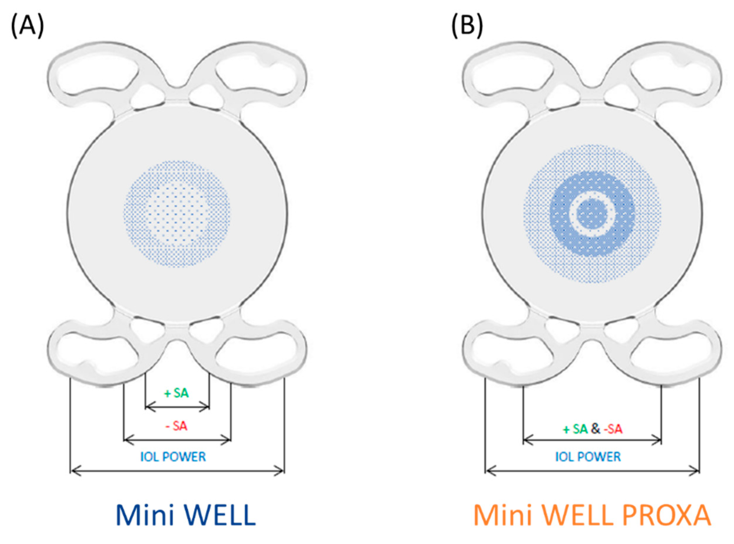
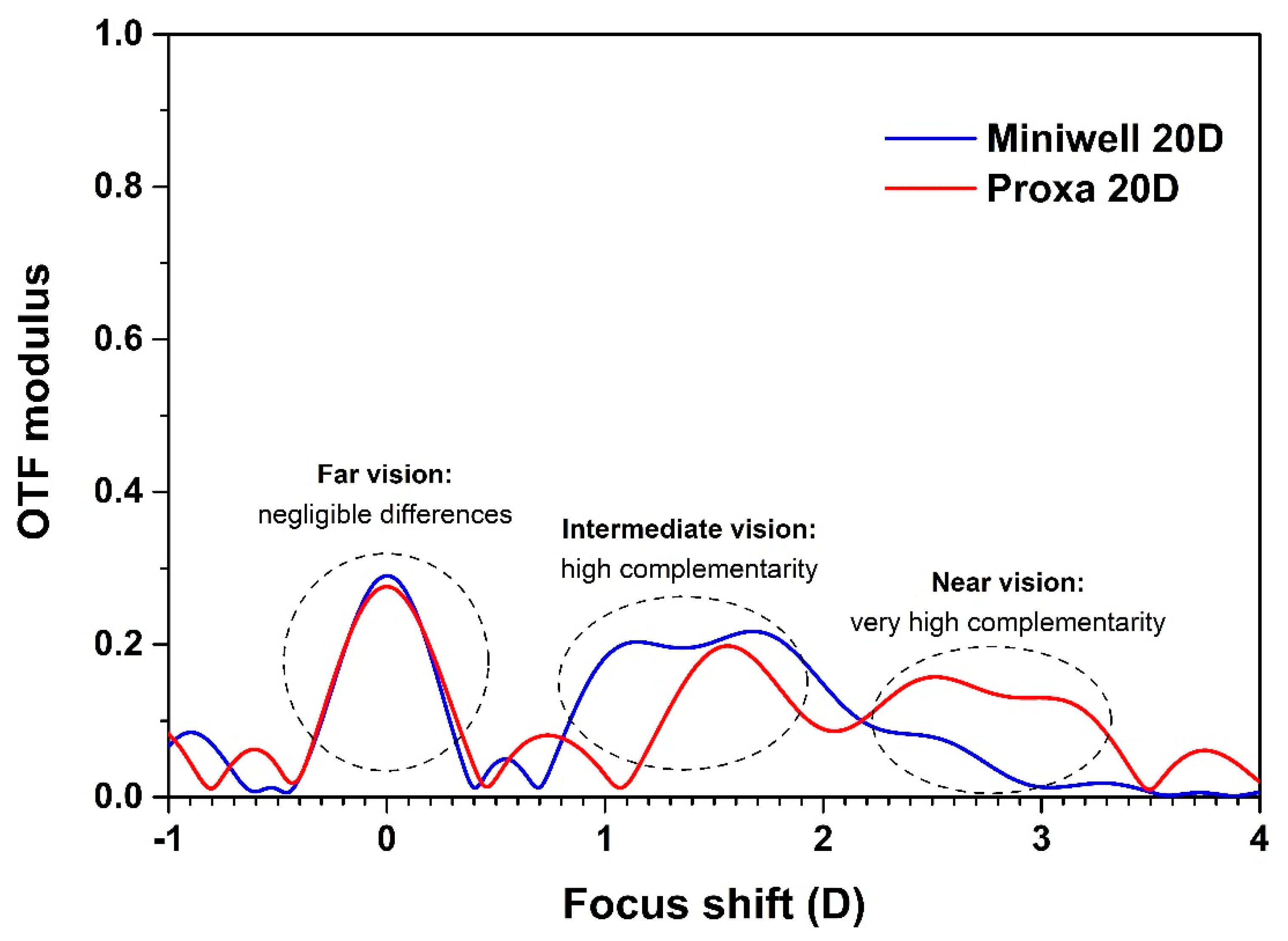
- Spanò, S.F.; Anastasi, E.; Frison, R.; Mazzone, M.G.; Curatolo, M.C. A new strategy in presbyopia correction: Mini well + mini well Proxa. In Proceedings of the 39th Congress of the European Society of Cataract and Refractive Surgeons (ESCRS), Amsterdam, The Netherlands, 8–11 October 2021. [Google Scholar]
- Kohnen, T. Nondiffractive Wavefront-Shaping Extended Range-of-Vision Intraocular Lens. J. Cataract Refract. Surg. 2020, 46, 1312–1313. [Google Scholar] [CrossRef] [PubMed]
- Mencucci, R.; Cennamo, M.; Venturi, D.; Vignapiano, R.; Favuzza, E. Visual Outcome, Optical Quality, and Patient Satisfaction with a New Monofocal IOL, Enhanced for Intermediate Vision: Preliminary Results. J. Cataract Refract. Surg. 2020, 46, 378–387. [Google Scholar] [CrossRef]
- Domínguez-Vicent, A.; Esteve-Taboada, J.J.; del Águila-Carrasco, A.J.; Ferrer-Blasco, T.; Montés-Micó, R. In Vitro Optical Quality Comparison between the Mini WELL Ready Progressive Multifocal and the TECNIS Symfony. Graefe’s Arch. Clin. Exp. Ophthalmol. 2016, 254, 1387–1397. [Google Scholar] [CrossRef]
- Nowik, K.E.; Nowik, K.; Kanclerz, P.; Szaflik, J.P. Clinical Performance of Extended Depth of Focus (EDOF) Intraocular Lenses—A Retrospective Comparative Study of Mini Well Ready and Symfony. Clin. Ophthalmol. 2022, 16, 1613–1621. [Google Scholar] [CrossRef]
- Rosa, N.; de Bernardo, M.; Lanza, M.; Borrelli, M.; Fusco, F.; Flagiello, A. Corneal Aberrations Before and after Photorefractive Keratectomy. J. Optom. 2008, 1, 53–58. [Google Scholar] [CrossRef] [Green Version]
- Wallerstein, A.A. Wavefront-Guided Refractive Surgery. Tech. Ophthalmol. 2003, 1, 17–19. [Google Scholar] [CrossRef] [Green Version]
- Camellin, M.; Mosquera, S.A. Simultaneous Aspheric Wavefront-Guided Transepithelial Photorefractive Keratectomy and Phototherapeutic Keratectomy to Correct Aberrations and Refractive Errors after Corneal Surgery. J. Cataract Refract. Surg. 2010, 36, 1173–1180. [Google Scholar] [CrossRef] [PubMed]
- Smadja, D.; Reggiani-Mello, G.; Santhiago, M.R.; Krueger, R.R. Wavefront Ablation Profiles in Refractive Surgery: Description, Results, and Limitations. J. Refract. Surg. 2012, 28, 224–232. [Google Scholar] [CrossRef] [PubMed] [Green Version]
- Mrochen, M.; Donitzky, C.; Wüllner, C.; Löffler, J. Wavefront-Optimized Ablation Profiles. J. Cataract Refract. Surg. 2004, 30, 775–785. [Google Scholar] [CrossRef] [PubMed]
- Manns, F.; Ho, A.; Parel, J.-M.; Culbertson, W. Ablation Profiles for Wavefront-Guided Correction of Myopia and Primary Spherical Aberration. J. Cataract Refract. Surg. 2002, 28, 766–774. [Google Scholar] [CrossRef]
- Cogan, D.G.; Toussaint, D.; Kuwabara, T. Retinal Vascular Patterns. Arch. Ophthalmol. 1961, 66, 366–378. [Google Scholar] [CrossRef]
- McWhirter, J.L.; Noguchi, H.; Gompper, G. Flow-Induced Clustering and Alignment of Vesicles and Red Blood Cells in Microcapillaries. Proc. Natl. Acad. Sci. USA 2009, 106, 6039–6043. [Google Scholar] [CrossRef] [Green Version]
- Zhong, Z.; Petrig, B.L.; Qi, X.; Burns, S.A. In Vivo Measurement of Erythrocyte Velocity and Retinal Blood Flow Using Adaptive Optics Scanning Laser Ophthalmoscopy. Opt. Express 2008, 16, 12746–12756. [Google Scholar] [CrossRef]
- Guevara-Torres, A.; Joseph, A.; Schallek, J.B. Label Free Measurement of Retinal Blood Cell Flux, Velocity, Hematocrit and Capillary Width in the Living Mouse Eye. Biomed. Opt. Express 2016, 7, 4228–4249. [Google Scholar] [CrossRef] [Green Version]
- Polans, J.; Cunefare, D.; Cole, E.; Keller, B.; Mettu, P.S.; Cousins, S.W.; Allingham, M.J.; Izatt, J.A.; Farsiu, S. Enhanced Visualization of Peripheral Retinal Vasculature with Wavefront Sensorless Adaptive Optics Optical Coherence Tomography Angiography in Diabetic Patients. Opt. Lett. 2017, 42, 17–20. [Google Scholar] [CrossRef]
- Chui, T.Y.P.; Zhong, Z.; Song, H.; Burns, S.A. Foveal Avascular Zone and Its Relationship to Foveal Pit Shape. Optom. Vis. Sci. 2012, 89, 602–610. [Google Scholar] [CrossRef] [PubMed] [Green Version]
- Tam, J.; Roorda, A. Speed Quantification and Tracking of Moving Objects in Adaptive Optics Scanning Laser Ophthalmoscopy. J. Biomed. Opt. 2011, 16, 036002. [Google Scholar] [CrossRef] [PubMed] [Green Version]
- Salmon, A.E.; Cooper, R.F.; Langlo, C.S.; Baghaie, A.; Dubra, A.; Carroll, J. An Automated Reference Frame Selection (ARFS) Algorithm for Cone Imaging with Adaptive Optics Scanning Light Ophthalmoscopy. Transl. Vis. Sci. Technol. 2017, 6, 9. [Google Scholar] [CrossRef] [PubMed] [Green Version]
- Gofas-Salas, E.; Mecê, P.; Mugnier, L.; Bonnefois, A.M.; Petit, C.; Grieve, K.; Sahel, J.; Paques, M.; Meimon, S. Near Infrared Adaptive Optics Flood Illumination Retinal Angiography. Biomed. Opt. Express 2019, 10, 2730–2743. [Google Scholar] [CrossRef] [Green Version]
- Piñero, D.P.; Cabezos, I.; López-Navarro, A.; de Fez, D.; Caballero, M.T.; Camps, V.J. Intrasession Repeatability of Ocular Anatomical Measurements Obtained with a Multidiagnostic Device in Healthy Eyes. BMC Ophthalmol. 2017, 17, 193. [Google Scholar] [CrossRef]
- Gordon-Shaag, A.; Piñero, D.P.; Kahloun, C.; Markov, D.; Parnes, T.; Gantz, L.; Shneor, E. Validation of Refraction and Anterior Segment Parameters by a New Multi-Diagnostic Platform (VX120). J. Optom. 2018, 11, 242–251. [Google Scholar] [CrossRef]
- Hénault, F.; Spang, A.; Feng, Y.; Schreiber, L. Crossed-Sine Wavefront Sensor for Adaptive Optics, Metrology and Ophthalmology Applications. Eng. Res. Express 2020, 2, 015042. [Google Scholar] [CrossRef]
- Pelzman, C.; Cho, S.-Y. Wavefront Detection Using Curved Nanoscale Apertures. Appl. Phys. Lett. 2019, 114, 183103. [Google Scholar] [CrossRef]
- Teperik, T.V.; Archambault, A.; Marquier, F.; Greffet, J.J. Huygens-Fresnel Principle for Surface Plasmons. Opt. Express 2009, 17, 17483–17490. [Google Scholar] [CrossRef] [Green Version]
- Luo, X. Subwavelength Optical Engineering with Metasurface Waves. Adv. Opt. Mater. 2018, 6, 1701201. [Google Scholar] [CrossRef]
- Zhang, S.; Wong, C.L.; Zeng, S.; Bi, R.; Tai, K.; Dholakia, K.; Olivo, M. Metasurfaces for Biomedical Applications: Imaging and Sensing from a Nanophotonics Perspective. Nanophotonics 2020, 10, 259–293. [Google Scholar] [CrossRef]
- Decker, M.; Staude, I.; Falkner, M.; Dominguez, J.; Neshev, D.N.; Brener, I.; Pertsch, T.; Kivshar, Y.S. High-Efficiency Dielectric Huygens’ Surfaces. Adv. Opt. Mater. 2015, 3, 813–820. [Google Scholar] [CrossRef] [Green Version]
- Pfeiffer, C.; Grbic, A. Metamaterial Huygens’ Surfaces: Tailoring Wave Fronts with Reflectionless Sheets. Phys. Rev. Lett. 2013, 110, 197401. [Google Scholar] [CrossRef] [PubMed] [Green Version]
- Chong, K.E.; Staude, I.; James, A.; Dominguez, J.; Liu, S.; Campione, S.; Subramania, G.S.; Luk, T.S.; Decker, M.; Neshev, D.N.; et al. Polarization-Independent Silicon Metadevices for Efficient Optical Wavefront Control. Nano Lett. 2015, 15, 5369–5374. [Google Scholar] [CrossRef] [PubMed]
- Shalaev, M.I.; Sun, J.; Tsukernik, A.; Pandey, A.; Nikolskiy, K.; Litchinitser, N.M. High-Efficiency All-Dielectric Metasurfaces for Ultracompact Beam Manipulation in Transmission Mode. Nano Lett. 2015, 15, 6261–6266. [Google Scholar] [CrossRef] [PubMed]
- Ballantine, K.E.; Ruostekoski, J. Cooperative Optical Wavefront Engineering with Atomic Arrays. Nanophotonics 2021, 10, 1901–1909. [Google Scholar] [CrossRef]
- Ang, M.; Gatinel, D.; Reinstein, D.Z.; Mertens, E.; Alió del Barrio, J.L.; Alió, J.L. Refractive Surgery beyond 2020. Eye 2021, 35, 362–382. [Google Scholar] [CrossRef]
- Ianchulev, T.; Hoffer, K.J.; Yoo, S.H.; Chang, D.F.; Breen, M.; Padrick, T.; Tran, D.B. Intraoperative Refractive Biometry for Predicting Intraocular Lens Power Calculation after Prior Myopic Refractive Surgery. Ophthalmology 2014, 121, 56–60. [Google Scholar] [CrossRef]
- Spekreijse, L.S.; Bauer, N.J.C.; van den Biggelaar, F.J.H.M.; Simons, R.W.P.; Veldhuizen, C.A.; Berendschot, T.T.J.M.; Nuijts, R.M.M.A. Predictive Accuracy of an Intraoperative Aberrometry Device for a New Monofocal Intraocular Lens. J. Cataract Refract. Surg. 2022, 48, 542–548. [Google Scholar] [CrossRef]
- Gasparian, S.A.; Nassiri, S.; You, H.; Vercio, A.; Hwang, F.S. Intraoperative Aberrometry Compared to Preoperative Barrett True-K Formula for Intraocular Lens Power Selection in Eyes with Prior Refractive Surgery. Sci. Rep. 2022, 12, 7357. [Google Scholar] [CrossRef]
- Krueger, R.R.; Shea, W.; Zhou, Y.; Osher, R.; Slade, S.G.; Chang, D.F. Intraoperative, Real-Time Aberrometry During Refractive Cataract Surgery With a Sequentially Shifting Wavefront Device. J. Refract. Surg. 2013, 29, 630–635. [Google Scholar] [CrossRef] [PubMed]
- Packer, M. Effect of Intraoperative Aberrometry on the Rate of Postoperative Enhancement: Retrospective Study. J. Cataract Refract. Surg. 2010, 36, 747–755. [Google Scholar] [CrossRef] [PubMed]


| IOL Material | Sphericity Status | Hygroscopy (%) | Glass Transition Temperature (°C) | Refractive Index (n) |
|---|---|---|---|---|
| Collamer | Negative | 40 | 40 | 1.44 |
| Hydrophobic acrylic | Spherical | 0.1–0.5 | 16–55 | 1.47–1.56 |
| Hydrophilic acrylic | Neutral | 18–38 | 10–20 | 1.40–1.43 |
| PEG-PEA/HEMA/Styrene copolymer | Neutral | 4–5 | 28 | 1.54 |
| PMMA | Negative | 0.4–0.8 | 105–113 | 1.49 |
| Silicone | Neutral | 0.38 | −90–−120 | 1.43 |
Publisher’s Note: MDPI stays neutral with regard to jurisdictional claims in published maps and institutional affiliations. |
© 2022 by the authors. Licensee MDPI, Basel, Switzerland. This article is an open access article distributed under the terms and conditions of the Creative Commons Attribution (CC BY) license (https://creativecommons.org/licenses/by/4.0/).
Share and Cite
Vacalebre, M.; Frison, R.; Corsaro, C.; Neri, F.; Conoci, S.; Anastasi, E.; Curatolo, M.C.; Fazio, E. Advanced Optical Wavefront Technologies to Improve Patient Quality of Vision and Meet Clinical Requests. Polymers 2022, 14, 5321. https://doi.org/10.3390/polym14235321
Vacalebre M, Frison R, Corsaro C, Neri F, Conoci S, Anastasi E, Curatolo MC, Fazio E. Advanced Optical Wavefront Technologies to Improve Patient Quality of Vision and Meet Clinical Requests. Polymers. 2022; 14(23):5321. https://doi.org/10.3390/polym14235321
Chicago/Turabian StyleVacalebre, Martina, Renato Frison, Carmelo Corsaro, Fortunato Neri, Sabrina Conoci, Elena Anastasi, Maria Cristina Curatolo, and Enza Fazio. 2022. "Advanced Optical Wavefront Technologies to Improve Patient Quality of Vision and Meet Clinical Requests" Polymers 14, no. 23: 5321. https://doi.org/10.3390/polym14235321