Article

Uncertainties in Electric Circuit Analysis of Anisotropic Electrical Conductivity and Piezoresistivity of Carbon Nanotube Nanocomposites

Center for Petroleum Science and Engineering, Skolkovo Institute of Science and Technology, 121205 Moscow, Russia
*
Author to whom correspondence should be addressed.
Polymers 2022, 14(22), 4794; https://doi.org/10.3390/polym14224794
Submission received: 21 September 2022 / Revised: 27 October 2022 / Accepted: 28 October 2022 / Published: 8 November 2022

Abstract

:
Electrical conductivity and piezoresistivity of carbon nanotube (CNT) nanocomposites are analyzed by nodal analysis for aligned and random CNT networks dependent on the intrinsic CNT conductivity and tunneling barrier values. In the literature, these parameters are assigned with significant uncertainty; often, the intrinsic resistivity is neglected. We analyze the variability of homogenized conductivity, its sensitivity to deformation, and the validity of the assumption of zero intrinsic resistivity. A fast algorithm for simulation of a gauge factor is proposed. The modelling shows: (1) the uncertainty of homogenization caused by the uncertainty in CNT electrical properties is higher than the uncertainty, caused by the nanocomposite randomness; (2) for defect-prone nanotubes (intrinsic conductivity ~104 S/m), the influence of tunneling barrier energy on both the homogenized conductivity and gauge factor is weak, but it becomes stronger for CNTs with higher intrinsic conductivity; (3) the assumption of infinite intrinsic conductivity (defect-free nanotubes) has strong influence on the homogenized conductivity.

Graphical Abstract

1. Introduction

Prediction of the electrical properties of nanocomposites, in particular with carbon nanotubes (CNTs) as a filler, includes simulations of homogenized conductivity and piezoresistivity (change in the homogenized conductivity with deformation of nanocomposite), given the volume fraction and architecture of CNTs and their electrical properties. Nodal analysis of the conductive resistor network formed by CNTs above the percolation threshold in an insulative matrix is a well-established method for the simulation of the homogenized electrical conductivity of CNT-filled polymers. The resistor networks model [1] was applied to CNT nanocomposites in early 2000 [2,3,4]. In the next decades up to the present, these models were further developed in numerous publications, mostly based on random generation of a CNT assembly with its subsequent transformation into a resistor network (to name a few, [5,6,7,8,9,10,11,12,13,14,15]) or with alternative formulations of charge flow [16] and micromechanics-type calculations of homogenized conductivity [17,18,19]. The resistor network approach was further used as a basis for models of piezoresistive behavior for CNT nanocomposites [20,21,22,23,24,25,26,27]. Availability of such models opened a way for multi-scale simulations of CNT nanocomposites [28] and the optimization of sensing simulations based on complex machine learning algorithms [29], in line with micromechanical toughness optimization methods [30,31].
As in any simulation, the adequacy of any property prediction depends on the adequacy of input data. For the conductivity of CNT nanocomposites at a given volume fraction of the filler, the input includes (1) geometrical characteristics of CNTs (single- or multiwalled and the wall count, outer diameter, and length distribution), (2) their waviness, (3) geometrical characteristics of the CNT assembly (orientation distribution, and level of agglomeration), and finally, (4) the electrical characteristics of CNTs and their contacts. Apart from the number of walls and the CNT diameter, all these parameters for a given material are neither readily available from manufacturer’s datasheets, nor easily measurable, nor, at least, fully evaluated. Therefore, input data create a very considerable uncertainty, which should be accounted for in the results of calculations (i.e., propagation of error).
The present paper is dedicated to the electrical characteristics of CNTs and their contacts. It analyzes the uncertainty of the choice of parameters, including the intrinsic conductivity of CNTs themselves (up to an assumption of zero resistance of CNTs, the so-called ballistic limit) and tunneling conductivity of their contacts, plus the uncertainty of the following nodal analysis. This complex uncertainty has not been given proper attention in the literature, including works cited above; the authors provide reasons for their choice of a certain dataset but very rarely discuss possible deviations from the chosen values. Study [32] conducted an analysis of prediction variations in a simplified model of randomly oriented CNT networks depending on the chosen values of the intrinsic and tunneling conductivity. Recently published research [33] presents a statistical analysis of electro-mechanical properties of CNT nanocomposites, including conductivity and piezoresistivity, using micromechanical modelling of parallel arrays of CNTs for a wide range of tunneling energy barrier values and for a fixed value of the intrinsic CNT conductivity.
We will analyze (1) the range of variations for the conductivity tensor and its deformation sensitivity resulting from the nodal analysis and caused by the uncertainty of parameters, namely the intrinsic and tunneling CNT conductivities, and (2) the credibility limits for the assumption of the zero CNT intrinsic resistivity for two cases of the nanocomposite internal structure: isotropically oriented assembly of CNTs, resulting in an isotropic conductivity tensor, and aligned CNTs, leading to anisotropic conductivity.
Numerical simulations in this work are accomplished using Matlab version R2020a.

2. Uncertainty in Electrical Conductivity as Input Data

2.1. Intrinsic CNT Conductivity

2.1.1. Physical Phenomena

Theoretically, the resistances of an ideal single-walled CNT (SWCNT) and a multi-walled CNT (MWCNT) are quantum (the so-called ballistic electron transport) which do not depend on the length of the conductive segment if this length is smaller than the mean free path of electrons. The latter is theoretically estimated as ~1 µm for SWCNTs and tens of micrometers for MWCNTs [34]. The typical distance b between CNT contacts along a CNT in a random CNT assembly can be estimated as b = d / 2 V f [35,36], where d is the CNT diameter, and Vf is the volume fraction. For typical values d ~ 0.01 µm and Vf ~ 0.01, this equation gives b ~ 0.5 µm, which is shorter than 1 µm of the free path. This suggests that the conductivity along CNT segments between two contact points should be taken as ballistic, and there exist experimental data supporting this statement [37,38,39]. However, the reliability of these measurements has been strongly criticized. Studies [40,41] argued that the used liquid–metal contact method gives “false positive” results for the ballistic nature of conductance. The theory of quantum resistance assumes the absence of the CNT structural defects. This assumption, although better justified on nano-scale than on macro-scale, still oversimplifies the description of the reality since CNT defects are experimentally observed and well-studied [42,43,44]. The presence of defects causes electron scattering and, thereby, the degradation of their mean free path length. For example, in [44] the mean free path length in MWCNTs was measured to be just 4.7 nm, which is a thousand times shorter than the theoretically suggested value for the ideal defect-free case. The authors of [44] suggested that the presence of defects cause a diffusive, Ohmic type of resistance, linearly increasing with the increase in the length of a conducting segment.

2.1.2. Implementation in the Nodal Analysis

In the nodal analysis of CNT networks, there exist two approaches (see the references below in this section). The first assumes the Ohmic proportionality of the resistance of a CNT segment to its length, taking both intrinsic and tunneling resistances into account. The second approach assumes infinite conductivity along the CNTs, constructing a network of only the inter-CNT contacts.
With the first approach, conductance GCNT of a CNT segment of length lseg is calculated as:
G C N T = g i n t r A l s e g
where A is the CNT cross-sectional area, and gintr is the volumetric conductivity of the CNT. The area is most often taken as the full area of the cross section, A = π d 2 / 4 , where d is the outer CNT diameter. This definition is also often used when processing experimental data. In several experimental and modelling works, the presence of the internal hole is accounted for in calculations of the area A. Using the empirical link between the CNT diameter and the number of walls Nw = (d[nm]−1) [45], the difference between the tubular and the full cross-section area can be estimated; it is in the range 10–20% for 5 < d < 35 nm. In the following, the full area of the cross section will be used; hence, gintr has the meaning of the effective volumetric conductivity; if a literature source relied on the tubular cross section, the data were re-calculated.
Figure 1a shows the results of measurements of gintr reported by [46] (measurement on single SWCNTs), [47,48] (single MWCNTs), and [44,49,50] (MWCNTs, aligned assembly). Even in the same series of experiments, the difference in gintr can be as large as 50 times. There exists a weak negative correlation between gintr and the CNT diameter (experimental data in Figure 1a); one can speculate that this is the result of a higher defect content in larger diameter CNTs. The CNT manufacturers do not provide data on CNT conductivity in their datasheets; an exception is MWCNTs NC7000, where the value, shown in Figure 1a (“internal test method” is referenced) is given in [51].
The popular choices of gintr for analyses of CNT networks are round values 103 S/m [33], 104 S/m [3,4,6,7,8,9,22], and 106 S/m [10,15]. In these sources, no detailed arguments were given for the choice of this parameter, apart from a reference to the general range of it (through three decimal orders of magnitude). Studies of the influence of this choice have not been conducted, apart from the work [32], where the range 103–106 S/m is explored.
The reality is even more complex. Any individual CNT will have conductivity affected by chirality and defects, creating a distribution of gintr. All of these distributions are unquantified, to the best of authors’ knowledge.
As mentioned above, in a number of modelling studies [12,24,26,27,52,53,54,55], the conductance of CNT segments in a network was taken to be infinite, with the network conductance defined by the contacts (tunneling currents). The differences in homogenized conductivity calculated with this assumption and with finite conductivity of CNTs were not assessed in detail.
Based on the review in this subsection, we will investigate differences in the nodal analysis of a CNT network for the levels of the effective CNT conductivity between 104 S/m and 106 S/m. The level of 108 S/m will be taken as very high, producing almost the same results as an assumption of infinite conductivity.

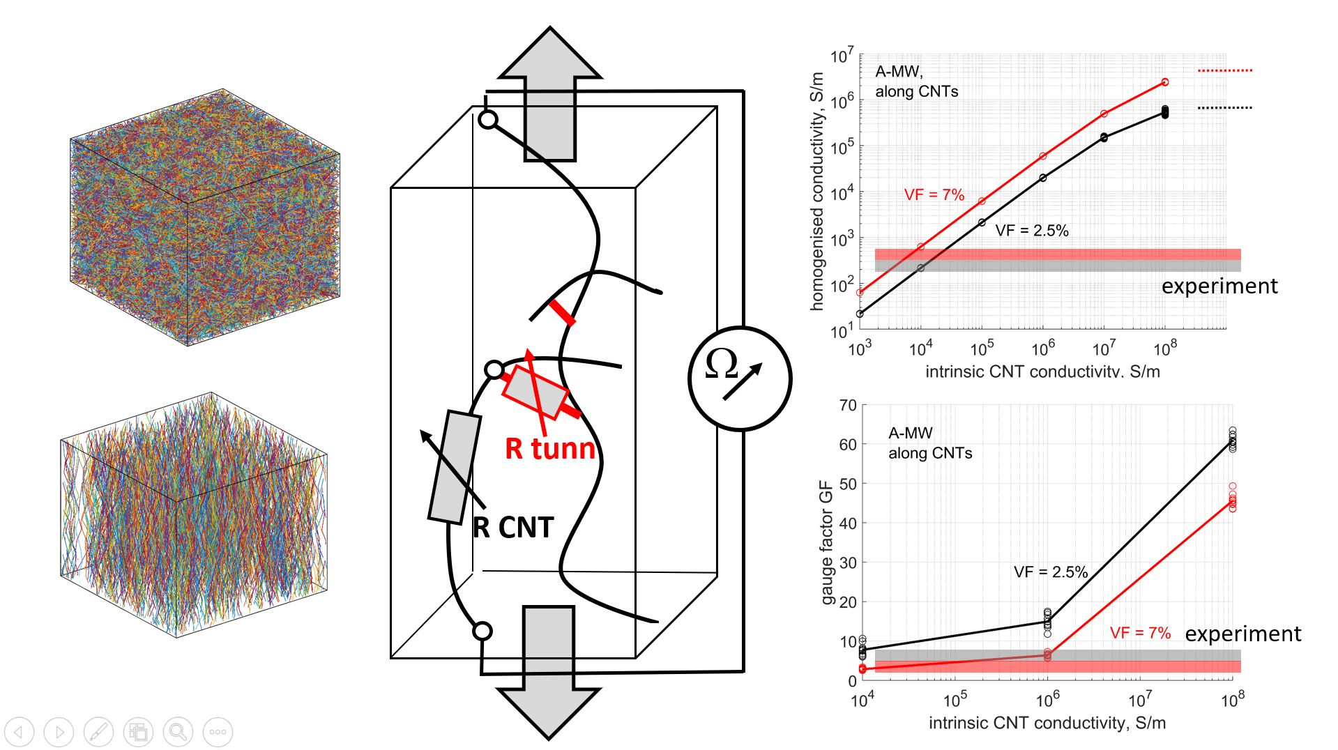
2.2. Tunneling Conductance of CNT Contacts

2.2.1. Simmons’ Formula

The contact conductance between CNTs is governed by the fluctuation-induced tunneling electron transport [56] and depends on the probability of electrons to overcome the electric potential barrier between CNTs. The tunneling conductance can be described with Simmons’ formula [57], which for low voltage on a contact is [58]:
G t u n n = G 0 τ s d 2 32 exp ( τ s )
where s is the distance between the CNT surfaces, ssmin, d is the CNT outer diameter, G 0 = 2 e 2 / h = 7.722⋅10−5 S (e = 1.602⋅10−19 C is electron’s charge, h = 6.626⋅10−34 J⋅s is Plank’s constant), and
τ = 4 π 2 m Δ E h
where m = 9.109⋅10−31 kg is the electron’s mass, and ΔE is the potential barrier.
Application of the low voltage variant of Simmons’ formula is justified by the fact that the dependence of tunneling conductivity on contact voltage is felt only if the voltage applied to the nanocomposite is extremely high, of the order of 1 V/µm and higher [59].
The value of smin is usually taken as 0.34 nm (van der Waals distance). It can be argued that adhesion between two nanotubes can decrease their minimal separation; for SWCNTs, the minimal distance caused by the adhesion was estimated as 0.25 nm [60].
The potential barrier ΔE is shown by [58] to have different values for the contact distances below and above the “polymer cutoff distance”, assumed to be 0.6 nm for polyethylene (PE) [58]. The same value, 0.6 nm, was used in [6,7,11,13] for epoxy as well and, in the absence of better estimations, is employed in the present calculations also. The difference between the potential barrier values below and above the polymer cutoff distance is attributed in [58] to a result of atomistic modelling. For a wider gap between the CNTs, the PE molecule penetrates into the gap, causing the decrease in the barrier height due to the resonance between tails of CNT wave functions and frontier orbitals in the PE molecule and leading to that for a charge that is easier (more probable) to transfer over the polymer-filled gap than over a vacuum gap. The values of ΔE are calculated in [58] for PE as ΔE1 (s < 0.6 nm) = 4.5 eV and ΔE2 (s > 0.6 nm) = 3.0 eV. Other authors provide values for ΔE1 down to 0.5–2.5 eV [61] and up to 5 eV [62].

2.2.2. Number of Conductive Channels

Equation (2) is based on the approximation of an equivalent parallel-plate capacitor of area d 2 and separation s. An alternative formulation given by [63] and further used, for example, in [6,7,11,13], is:
G t u n n = G 0 M exp ( τ s )
where M is the number of channels for tunneling. M = 2 for SWCNTs and M = 400–500 for MWCNTs [64]. Value M = 450 is generally employed in calculations [6,7,11,13]. Equalizing coefficients in Equations (2) and (4) at s = 0.34 nm and ΔE = 1–5 eV, the equivalent values of M for a SWCNT with d = 1.6 nm can be computed to be in the range 2–5, and for an MWCNT with d = 15 nm to be in the range 200–500. Therefore, Equation (2) provides the results close to the simplified Equation (4) but explicitly accounting for the dependency of coefficient M on the inter-CNT distance and CNT diameter. In the present calculations, Equation (2) will be used.
For numerical experiments in the present work, we will investigate the differences in homogenized conductivity and deformation sensitivity of nanocomposites, which originate from the difference in assumed ΔE1 values, in the interval 1–5 eV. In addition, it will be assumed that ΔE2 = ΔE1/1.5, and the polymer cutoff distance is 0.6 nm (Figure 1b).

3. Geometrical and Electrical Models

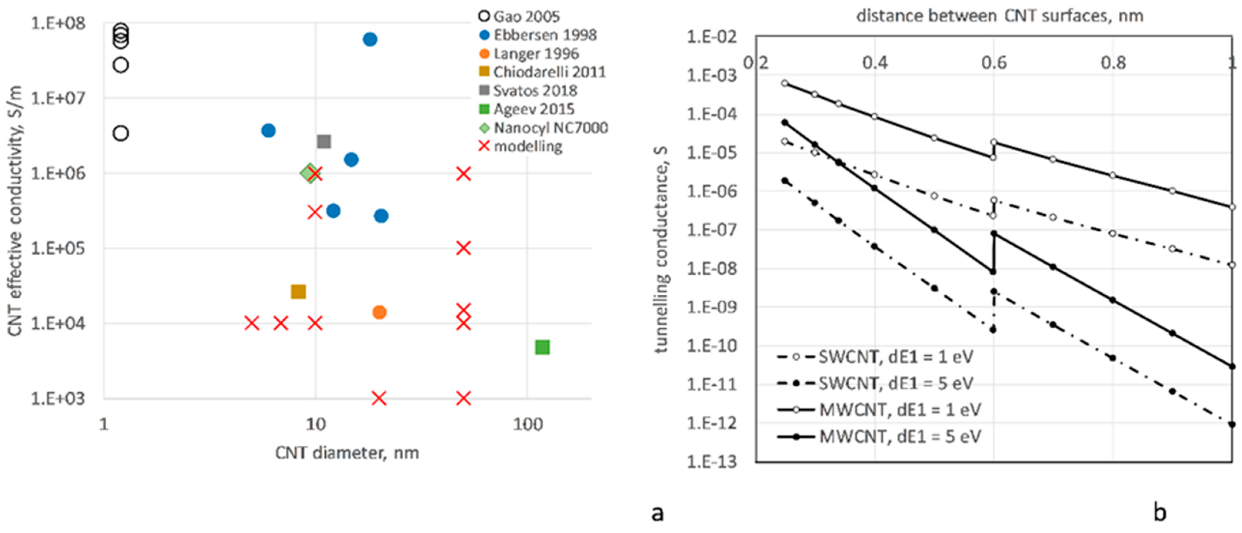
3.1. Geometrical Model

3.1.1. Variants of CNT Geometry

Two geometrical arrangements of a wavy CNT assembly are considered here: (1) isotropically randomly oriented, uniformly spatially dispersed SWCNTs (designated “R-SW” below) and (2) aligned MWCNT assembly (A-MW), with parameters given in Table 1. Both types of nanocomposites were previously experimentally studied by the present authors [65,66,67,68,69].

3.1.2. The Algorithm

The algorithm generating the geometrical model is described in [70,71] and is illustrated in Figure 2. It uses random choice of the direction of a generated CNT path segment, as is widely used in the literature, for example, in [72,73], but with certain constraints, as described below. Figure 2a shows a scheme of the nth segment of a CNT with length lseg, and orientation defined by the azimuthal angle φn and polar angle θn. To generate the aligned assembly, the angles φn and θn are defined in relation to the global Cartesian coordinate system of the assembly with axis z corresponding to the direction of forest growth. For generation of a random assembly, the angles are defined in the local coordinate system with axis z corresponding to the direction of the previous segment, where the first segment was oriented according to the uniform orientation distribution. The angles φn and θn are random values. They are first calculated as φn = rand(0,2π), cosθn = randN(1, cos(σθ)), where rand(a,b) is a random generator of the uniform distribution on [a,b], randN(a, σ) is a random generator of the normal distribution with mean a and standard deviation σ, and σθ is a characteristic polar angle deviation, which is calculated based on the length of the CNT segment and the maximal curvature. The randomness of segment orientation is restricted by the following conditions:
(1)
Maximal path curvature and torsion are limited: κ κ m a x ; τ τ m a x . This type of control was introduced recently in [71] that demonstrated, apart from adequate representation of CNT shapes, that these conditions suppress the segment length dependence of the homogenized conductivity. If for generated φn and θn the curvature and torsion do not satisfy these conditions, φn and θn are generated again;
(2)
Correlated random angles: the sequences of φn and θn pairs are auto-correlated along the CNT path, with the assumed correlation length of 100 nm (see [70]).
For the random assembly, the origins of CNT paths are distributed uniformly in the model volume, and initial orientations are distributed isotropically. For the aligned assembly, CNTs’ origins are placed randomly and uniformly on a plane, using a Poisson random process.
For both cases, geometric periodicity is assumed; the model is confined within a representative volume element (RVE). If a CNT crosses an RVE face, then it is continued from the opposite face until the full length of the CNT is reached. The number of CNTs in the model is defined based on the prescribed volume fraction (VF). Figure 2a,b show random instances of (a) R-SW and (b) A-MW RVEs.

3.2. Electrical Model: Homogenized Conductivity

Once an RVE is created, the geometrical network of a CNT assembly is analyzed for contacts between CNTs and then transformed into a set of nodes, connected by electrical resistances/conductances, which are assigned to the tunneling contacts according to Equations (2)–(3) and to the CNT sections between the contacts according to Equation (1). The electrical boundary conditions are periodical. The homogenized conductivity tensor is then calculated using the homogenization theory outlined in Appendix A. The identification of contacts and nodal analysis are described in more detail in Appendix B.

3.3. Electrical Model: Piezoresistive Response

3.3.1. Principles of the Model

At deformation, distances s of the tunneling contacts, Equation (2), are changing, causing the change in the tunneling part of conductivity. When modelled, care should be taken to apply correct values of potential barriers. As discussed in Section 2.2, in the undeformed state, the potential barrier ΔE1 is applied at distances shorter than the polymer cutoff distance 0.6 nm, while at larger distances the value of the potential barrier is switched to ΔE2. The reason behind this is that at distances between two CNTs larger than 0.6 nm, polymeric chains begin to penetrate into this gap, while at shorter distances it is prevented by van der Waals’ forces. When we apply deformation, the distances between CNTs change. However, since we consider only elastic polymers with no or little plasticity, we assume that no polymer interpenetrates the opening gaps, and the values of the potential barriers must be evaluated with the reference to the undeformed configuration. The following rules are followed:
(Rule 1): If at deformation the gap between two CNTs is opening and exceeds the polymer cutoff distance, the potential barrier still remains ΔE1.
On the contrary, when the gap is not opening, but closing, we expect van der Waals’ forces to push the polymer out of this gap, thereby changing the potential barrier. Hence:
(Rule 2): If at deformation the gap between two CNTs is closing and becomes shorter than the polymer cutoff distance, the potential barrier switches to ΔE1.
Finally, due to the lack of matrix plasticity, if CNTs are separated by a large distance, by default filled with polymer, no conformational changes, no matter how close moving one CNT to another, can form new contact points. Therefore, the third rule is:
(Rule 3): Pairs of contact points, at which tunneling is happening, stay unchanged at deformation, and in the deformed configuration, no search for new contact points is performed.
In the present algorithm, no contacts between CNTs are severed or moved along CNTs; only distances between CNTs change. In addition, no new contacts are created. Therefore, our modelling approach would be inapplicable to changes in the system of contacts in a dry filament assembly (e.g., buckypaper in case of CNT filaments or non-woven fibrous material without bonding). On the contrary, in our research, we are dealing with impregnated composite with quite limited applied strain range, where the presence of solid matrix prevents free creation of new contacts.

3.3.2. Calculation of Gauge Factor

The piezoresistive gauge factor (GF) for uniaxial tension deformation ε in direction i is defined as
G F = 1 ε g i i g i i ( ε ) g i i
where gii and g i i ( ε ) are ii diagonal components of the homogenized conductivity tensors before and after the deformation.
The range of GF values found in the literature is very wide. Review [74] and later publications, e.g., [65,75], provide the following data. For non-aligned CNT distributions, with weight percentage of CNT below 2%, the most often observed values are in the range 1–7. Some authors give GFs up to 20–30 [76,77]. For aligned CNTs, the range of GFs for deformation in the direction of the CNT alignment is 0.04–10.
The simplest approach to model the deformational sensitivity is to consider dilatational deformational state in tension, assuming that all distances s of the tunneling contacts, Equation (2), change proportionally to the applied deformation (iso-strain) as s’ = s(1 + ε). In this case, the result can be estimated without the necessity of numerical simulations. Indeed, since all distances are increased proportionally and the values of potential berries are unchanged (rule 1), all tunneling conductances at contacts will drop proportionally to
exp ( τ s ( 1 + ε ) ) exp ( τ s ) s s ( 1 + ε ) = exp ( τ s ε ) 1 + ε
Hypothesizing that the main contribution to the tunneling part of conductivity comes from distances shorter than the polymer cutoff distance (which will be proved later by Figure 3b), we can assume the value of τ in Equation (6) as being determined by ΔE1 = 4.5 eV, i.e., τ ~ 22 nm−1. For distances s between 0.34 and 0.6 nm and with ε = 0.01, we expect Equation (6) to be in the range from 0.87–0.93 with the GF of the tunneling part to be in the range from 7 to 13. This is the total GF in case of infinite intrinsic conductivity. For non-zero intrinsic resistivity, the GF will be lower. These values correspond to the experimental observations.
However, assuming a proportional increase in all tunneling distances, one assumes homogeneous deformation of a nanocomposite despite orders of magnitude difference in stiffness between CNTs and polymer. Therefore, for accurate analysis, conformational changes of CNTs must be considered. To avoid 3D finite-element simulations (see, e.g., [22]), we propose a simplified procedure, which calculates the change of the tunneling contact distances under the following assumptions:
  • Average deformation is transferred unchanged to sub-micrometer scale deformation elements around the contact points of CNTs;
  • Length of a CNT does not change during the deformation.
The details of the applied deformation algorithm are given in Appendix C. The reader is referred to [78] for details of validation of the piezoresistivity model against finite elements calculations.
After new tunneling distances are calculated, the corresponding tunneling conductances are re-assigned.

4. Results and Discussion

4.1. Random RVE Instances

4.1.1. RVE Sets and Orientation Distribution

Using the algorithm described in Section 3, the RVE sets are generated for R-SW and A-MW input data: 33 RVE instances of R-SW and 100 of A-MW. Examples of the RVEs are shown in Figure 2b,c. Potential differences are applied to all pairs on the opposite RVE faces in a sequence. After homogenized conductivity is calculated, this produces 99 independent values for principal conductivity tensor components for isotropic R-SW (33 RVE instances times 3 directions of the potential difference application), 100 and 200 independent values for Z-conductivity and X/Y-conductivity, respectively, for transversely isotropic A-MW, with Z being the direction of the CNT alignment.
The orientation tensors a for two particular RVE realizations, shown in Figure 2b,c, calculated based on averaging orientations of CNT segments, are
R - SW :   a = [ 0.346 0.005 0.014 0.005 0.318 0.004 0.014 0.004 0.336 ]
A - MW :   a = [ 0.037 0.0003 0.013 0.0003 0.037 0.0008 0.013 0.0008 0.926 ]
The tensor for R-SW corresponds to the isotropic orientation, and for A-MW, the orientation is concentrated near the z-axis, with the average angle of deviation estimated as acos ( a 33 ) = 15.7°. These orientations are characteristic for all calculated RVE instances, with diagonal tensor components for R-SW deviating from 1/3 not more than by 0.02 and the average deviation angle for A-MW lying in the range 14–16°.

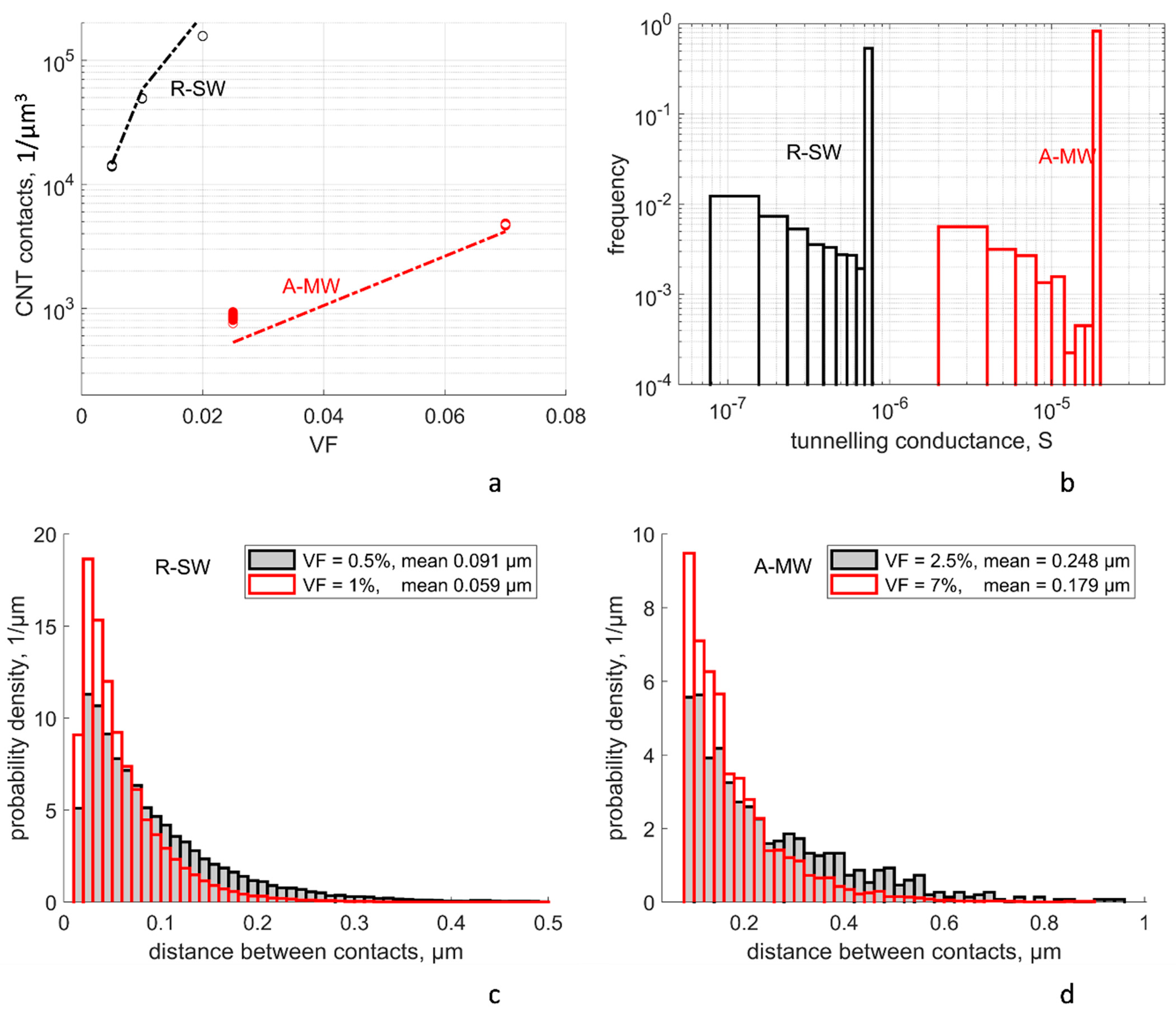
4.1.2. Distribution of CNT Contacts

The conductivity of an RVE depends on contact distances between CNTs, which, in turn, define the tunneling resistances of contacts and the conductivity of CNT segments between the contacts. These characteristics are shown in Figure 3.
Figure 3a shows the number of CNT contacts nc per 1 µm3 in the random RVEs as a function of CNT volume fraction VF (an additional value VF = 2% is added to the calculated variants of R-SW for comparison). The simulated values are compared in Figure 3a with a theoretical formula from [35,36]:
n c = 16 π 2 I V F 2 d C N T 3 k ,   where   k = d C N T + 0.0014   µ m d C N T
Here, dCNT is the CNT diameter, and I is an integral depending on the orientation distribution function; for isotropic distribution (R-SW), I = π/4, and for the distribution defined by the orientation tensor from Equation (7) for A-MW, I = 0.23, calculated using the formulae given in [35] for aligned wavy fibers. The correction coefficient k accounts for the fact that a contact is counted in the present simulations if the distance between CNT surfaces is in the range shorter than 1.4 nm, whilst in the theory, this contact distance is supposed to be zero. Comparison of the simulated values (dots in Figure 3a) with the theoretical trends shown by dashed lines, shows good correlation between the two. This allows us to conclude that the procedure for generation of CNT paths is consistent with general rules of geometry of random filament assemblies.
The scatter in the number of contacts for different random RVE realizations is minor (below ±10%) in all cases apart from the case of A-MW at low VF = 0.025; in the case of A-MW, the contact probability is defined by a combination of waviness-induced deviation of the CNT path from the straight vertical average line and a distance between these lines of adjacent CNTs, which is comparable to waviness deviations for low VF.
Each CNT contact is characterized by a contact distance between CNT surfaces, s. When the contacts are calculated, the distances dcentr between the CNT centerlines (paths) are determined. A contact defines a pair of points on the centerlines such that distance dcentr between them is smaller than the contact threshold of dCNT + 1.4 nm. The reader is referred to [71] for details of the contact calculations. Then, the distance between the CNT surfaces is calculated as
s = max ( s m i n , d c e n t r d C N T )
where smin is the minimal van der Waals distance between two CNTs (see Section 2.2). The majority of the contacts have dcentr < dCNT + smin, hence s = smin. The relative number of contacts with s > smin increases with s because of the increase of cylindrical volume with radius (dCNT + s, dCNT + s + Δs), where Δs is the width of the histogram bin.

4.1.3. Distribution of the Tunneling Conductances

Typical distributions of tunneling conductances of contacts are shown in Figure 3b for R-SW and A-MW cases. The overwhelming majority of contacts, 70–90%, are characterized by the maximal conductance, corresponding to the distance smin. The frequency of the histogram bins increases with the decrease in conductance value, corresponding to the increase of the relative number of contacts with higher s. The overall larger tunneling conductance in the MW case in comparison with SW corresponds to Equation (2) and curves shown in Figure 1b.
The tunneling resistance is compared with the mean resistance of CNT sections between the contacts (a distance between the contacts along a CNT). The distribution of lengths of these sections is shown in Figure 3c,d. Clearly, the mean values 60–90 nm for R-SW and 180–250 nm for A-MW are much larger than the characteristic defect-free length 4.7 nm [44]. Hence, CNT sections between two tunneling connections cannot be treated as defectless with the ballistic electron transport.
The mean inter-contact CNT resistance R C N T m e a n is calculated inverting Equation (1) with lseg = bmean, where bmean is the mean distance between two contacts along a CNT. The results of these calculations are plotted in Figure 4 (solid lines) as a dependency R C N T m e a n ~ ( g i n t r ) 1 for R-SW and A-MW cases, respectively. The levels for the tunneling resistance R t u n n 0.34 , which is an inversion of the tunneling conductance given by Equations (2) and (3), are plotted on the same graphs for the range of ΔE1 = 1–5 eV and the minimal distance between the CNT surfaces of 0.34 nm (which corresponds to the overwhelming portion of the contacts, see Figure 3b). Depending on the gintr value, the relation between two resistances can be different. For gintr ~ 104 S/m, R C N T m e a n > R t u n n 0.34 , and the CNT, intrinsic resistance defines the homogenized resistivity/conductivity. On the other end of the studied range, for gintr ~ 108 S/m, we have R C N T m e a n R t u n n 0.34 , and the tunneling resistance is the defining factor. In the middle of the gintr range, both resistances are comparable.

4.2. Plan of Numerical Experiments

To investigate the influence of the electrical conductivity input data on the homogenized RVE conductivity and deformation sensitivity, these parameters were calculated for random RVE instances, according to the plan of numerical experiments shown in Table 2. This plan investigates uncertainty of calculated performance characteristics of nanocomposites depending on (1) the uncertainty of setting the intrinsic conductivity of CNTs coupled with variation of the potential barrier for tunneling conductivity and (2) the uncertainty of the minimal (van der Waals) distance between CNTs (affected or not affected by CNT compression). The reference point of the plan is taken as
gintr = 104 S/m; ΔE1 = 3 eV; smin = 0.34 nm
which is the set of parameters most used in the modelling publications.

4.3. Uncertainty in Homogenized Conductivity

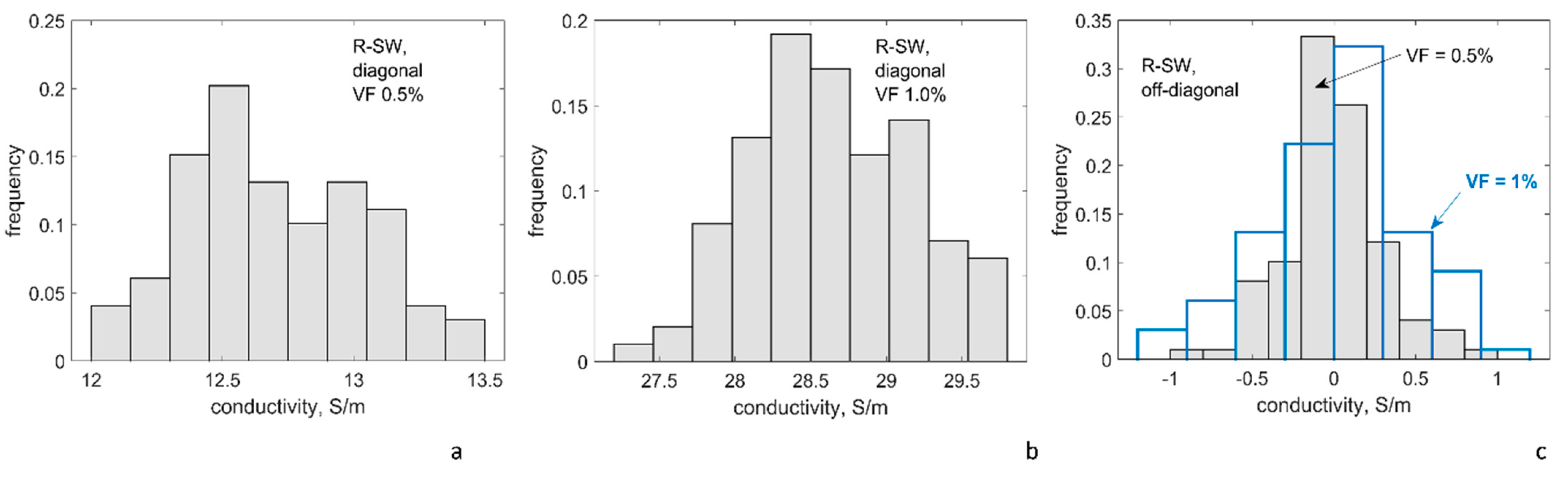
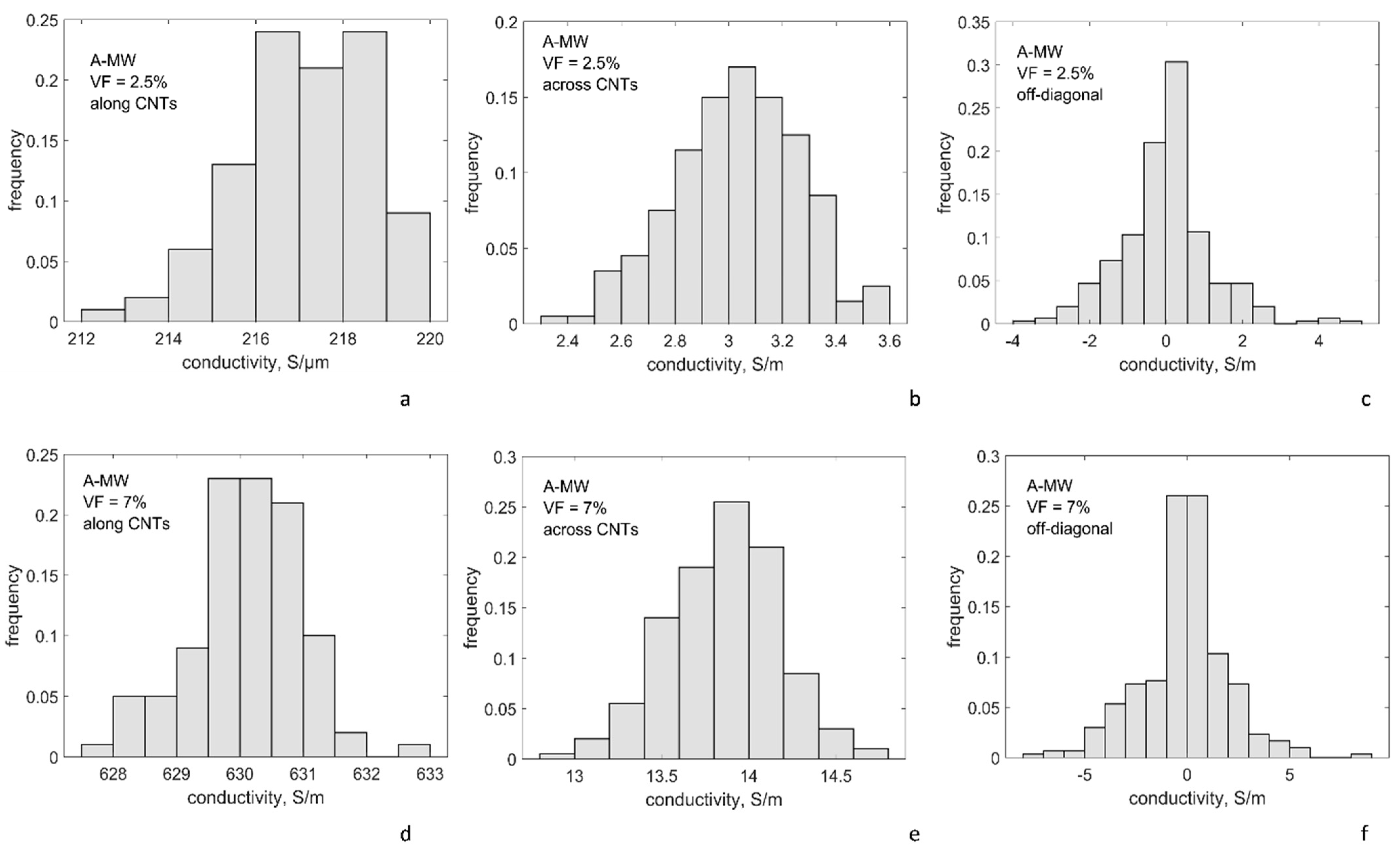
4.3.1. Conductivity at the Reference Point of the Plan for Numeric Experiments

Table 3 and Figure 5 and Figure 6 present the results of calculation of conductivity tensor for R-SW and A-MW configurations at the reference point of the plan for numerical experiments. Conductivity tensor G = [ G i j ]   (for its definition see Appendix A) is represented by the following group of values:
R-SW: This configuration is isotropic. Hence, all 3 diagonal components (G11, G22, G33) in all 33 random realizations of the RVE form a single sampling of 99 values; the same is valid for all 3 off-diagonal components (G12, G13, G23), which form a single sampling also with 99 values.
A-MW: This configuration is transversely isotropic. In all 100 random RVE realizations, conductivity along CNTs, G33, forms a sampling with size 100, conductivity across CNTs (G11, G22) forms a sampling with size 200, and for off-diagonal components (G12, G13, G23) a sampling with size 300 is formed.
The results of calculations present the expected dependency G(VF): with the CNT volume fraction above the percolation thresholds, both for R-SW and A-MW configurations, there is an increase of the homogenized conductivity with the increase of VF, but inside the same decimal order of magnitude of the conductivity values. This observation is typical post-percolation behavior well above the percolation threshold. The homogenized conductivity of A-MW in the CNT direction and across it differs by about 60 times.
The conductivity values, calculated using the reference point of the numerical plan (gintr = 104 S/m; ΔE1 = 3 eV; smin = 0.34 nm), are within one order of magnitude difference with the experimentally measured values for the R-SW system [65] and the A-MW system [69]. The comparison with the experiment will be discussed more in detail after the variability of modelling with variation of the input is investigated.
The scatter of the modelled conductivity values, shown in Table 3 and Figure 5, is caused by random RVE geometry variations. For the diagonal components, the coefficient of variation is just a few percent. This stability of the homogenized conductivity for volume fractions well above the percolation thresholds for both systems corresponds to a stability of the number of contacts, which is seen in Figure 3a. The general tendency can be observed: the denser the percolation network, the lower the scatter.

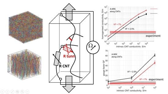
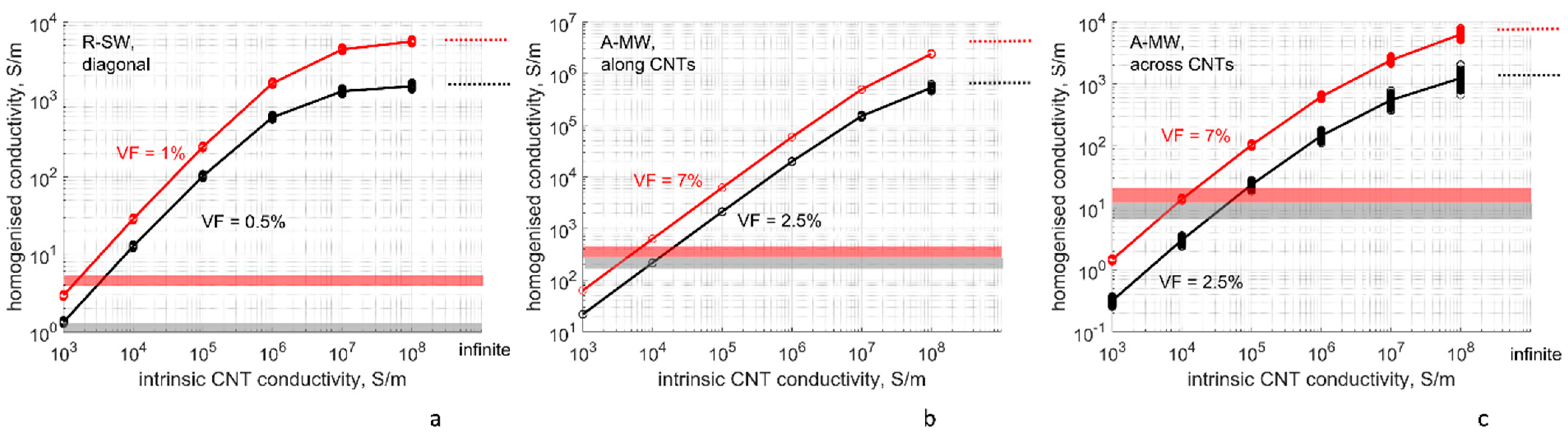
4.3.2. Dependency of the Homogenized Conductivity on the CNT Intrinsic Conductivity

Figure 7 shows results of simulations of the homogenized conductivity G (namely, different components of its tensor) for varying CNT intrinsic conductivity gintr. The other two variables of the numerical plan are kept constant at the reference values: ΔE1 = 3 eV, smin = 0.34 nm.
Figure 7 also shows a range of experimentally measured conductivity for R-SW and A-MW systems, reported by [65,69]. These ranges correspond to the results of the nodal analysis if the following values of gintr are assumed:
R-SW: gintr = (1–2)⋅103 S/m
A-MW: gintr = (0.7–2)⋅104 S/m
Varying the intrinsic conductivity by one decimal order of magnitude leads to a change in the homogenized conductivity also by one order of magnitude in all modelled configurations (isotropic R-SW, A-MW along and across the bundle). For the intrinsic conductivity range 103–106 S/m, the dependency G(gintr) is linear in log–log coordinates of Figure 7 and is described by a power law
G ( g i n t r ) p
where power p equals 0.833 ± 0.005 for diagonal components of R-SW, and 0.982 ± 0.007 (along CNTs), 0.827 ± 0.005 (across CNTs) for A-MW (least square fit). It is noteworthy that all three values are below unity (the difference is much higher than the scatter range) which can be expected from 3D percolation below the upper critical dimension. If gintr reaches high values of 107–108 S/m, the growth of the dependency G(gintr) is slowed with the values of G bounded by a maximum corresponding to the infinite intrinsic conductivity of CNTs (ballistic electron transport), shown by dashed lines in Figure 7a–c.
The strong influence of gintr on the homogenized conductivity, evidenced by Figure 7, means that accurate choice of gintr plays a paramount role in the qualitative success of modelling.
As shown in Section 2.1 (see Figure 1a), the experimentally measured values of intrinsic conductivity differ up to two orders of magnitude in different experiments. Experiments with single CNTs reported conductivities around 106 S/m for MWCNTs and near 108 S/m for SWCNTs. Experiments with CNT bundles lead to lower values around 104 S/m.
In numerical modelling (crosses in Figure 1a), in several cases, for example, [10,14,15], the value of 106 S/m was assumed. At the same time, [10] stated that this value, based on CNT manufacturer’s datasheet (Nanocyl point in Figure 1a), leads to a gross overestimation of the calculated conductivity in comparison with experimental data. Authors in [14,15] gave a reference to [47] (see Figure 1a) as a foundation for the choice gintr = 106 S/m for their modelling of carbon fibers/CNT hybrid composites. However, when comparing their calculations with experimental data on nanocomposites [79], with a good correspondence, [14,15] used a lower value gintr = 105 S/m.
Extremely high values, in the order of gintr = 108 S/m, measured by [46] for single SWCNTs (see Figure 1a), when put in the nodal analysis for an R-SW system (Figure 7a), led to the homogenized conductivity up to 103–104 S/m, VF = 0.5–1.0%. This is two to three orders of magnitude higher than values measured in [65,80,81,82].
Apparently, there is a contradiction between the results for intrinsic conductivity of CNTs obtained with experiments on single particles and with the correlations between experimentally measured conductivities of nanocomposites and their numerical counterparts. CNT aggregation and rope/bundle formation [83], absent in numerical studies, can cause the discrepancy between the predicted and experimentally measured conductivity of a nanocomposite, leading to the underestimation of the intrinsic conductivity. Therefore, we may hypothesize that in case of a detailed RVE modelling, with both agglomeration and bundling phenomena, values of the order of 106 S/m for MWCNTs and 108 S/m for SWCNTs may need to be implemented. However, implementation of these values in the modelling of as if perfectly dispersed and distributed particles (which corresponds to the present study) will certainly lead to the overestimation of the resulting conductivity.
Finally, for ordinary CNT production, the use of infinite conductivity looks like an oversimplification in spite of the considerable spread of this assumption [12,24,26,27,52,53,54,55]. Infinite CNT conductivity leads to the homogenized values several orders of magnitude higher in comparison with calculations implementing gintr = 104 S/m. However, the justification of the infinite intrinsic CNT conductivity can be argued by special conditions of CNT manufacturing, providing defect-free structure.

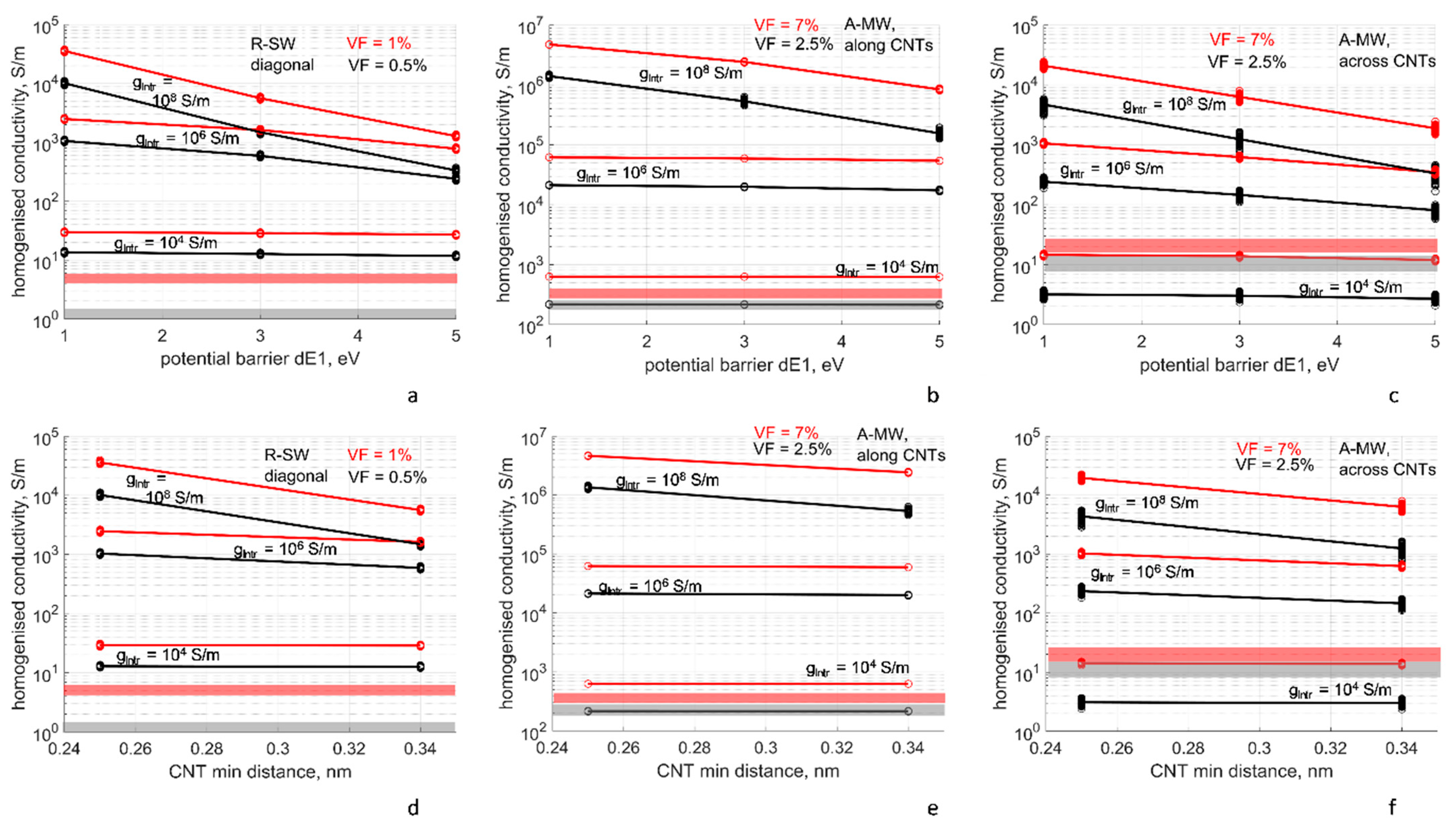
4.3.3. Dependency of the Homogenized Conductivity on the Tunneling Resistance Parameters and Minimal Inter-CNT Distance

Figure 8a–c show dependency of the homogenized conductivity GE1) on the potential barrier value ΔE1 of the tunneling conductance, Equations (2) and (3), for R-SW and A-MW cases at two levels of CNT volume fraction VF, and for three levels of the intrinsic CNT conductivity gintr, at smin = 0.34 nm. Behavior GE1) for different VFs is very similar: the homogenized conductivity decreases with the increase of ΔE1, the trend defined by the decrease of the tunneling conductance with increase of ΔE1, see Figure 1b.
The slope of GE1) depends on gintr. For gintr = 104 S/m, there is almost no dependency of G on ΔE1: it equals ~10% change in the range ΔE1 = 1–3 eV. The CNT segment resistance is higher than the tunneling resistance in this case (see Figure 3c,d), and the latter (defined by ΔE1) only weakly influences the homogenized conductivity.
For gintr = 106 S/m, the dependency GE1) becomes more pronounced. In the range ΔE1 = 1–3 eV, the homogenized conductivity changes by about five times for R-SW and A-MW across CNTs; in these two cases, the number of contacts on a percolating path is considerable. For gintr = 106 S/m, the CNT segment resistance and the tunneling resistance are in the same range and affect the homogenized conductivity collectively. For A-MW along CNTs, the change of GE1) over ΔE1 = 1–3 eV is minor, about 20%. This is explained by the fact that in the longitudinal direction of the bundle, there are only 2–3 contacts on the percolating path between two RVE sides, and the conductivity is defined by gintr, not tunneling.
The maximal slope of GE1) is reached at extremely high gintr = 108 S/m, which is almost equivalent to the infinite CNT conductivity assumption (see Figure 7). For this case, the CNT segment resistance is much lower than the tunneling resistance, Figure 4. The resistance of a percolating path is defined by resistances of tunneling contacts included in the path and hence strongly depends on ΔE1. GE1) changes over ΔE1 = 1–3 eV by 10 (A-MW) to 50 (R-SW) times.
Figure 8d–f show dependency of the homogenized conductivity GE1) on the minimal inter-CNT distance smin, for R-SW and A-MW cases at two levels of the CNT volume fraction VF and for three levels of the intrinsic CNT conductivity gintr, at ΔE1 = 3 eV; smin has two levels: smin = 0.34 nm, which is van der Waals distance, and 0.25 nm, given by [60] as a result of CNT lateral compression. Change in smin is equivalent to change of Δ E 1 (see Equations (2) and (3)); hence, there is no surprise that the curves in Figure 8d–f show the behavior very similar to Figure 8a–c. Varying the minimal inter-CNT distance is felt only in the case of very high gintr.
A practical conclusion can be drawn from our modeling observations. If non-infinite intrinsic CNT conductivity is assumed, with a value from the range 104–106 S/m, then the choice of ΔE1 value (in the range 1–5 eV) does not significantly affect the homogenized conductivity. In contrast, if there are reasons to assume infinite (very high) intrinsic CNT conductivity (defectless CNTs), then the choice of ΔE1 affects the calculated homogenized conductivity strongly. The similar conclusions were reached in studies of conductivity of CNT films [84] and for random CNT assemblies with Vf < 2% in [32], but further experimental observations are desired since it contradicts experimental evidence and theoretical arguments on the generally prevailing role of the tunneling conductivity [12,85].
The relative influence of the intrinsic conductivity and tunneling barrier parameters plays an important role when temperature dependence of nanocomposites conductivity is being discussed. Both random and aligned nanocomposites exhibit negative temperature coefficients of resistance (TCR), with resistivity decreasing by 5–15% when temperature increases from room temperature to 400–500 K [84,85,86,87,88]; the same behavior was noted in nanoplatelet networks [89,90]. This decrease in resistivity is governed by temperature dependence of both factors defining the homogenized conductivity: the tunneling resistance [85,90,91] and the intrinsic conductivity [34,91], combined with the thermal expansion. Further experimental evidence and a model of such processes are yet to be discovered.

4.4. Uncertainty of Deformation Sensitivity

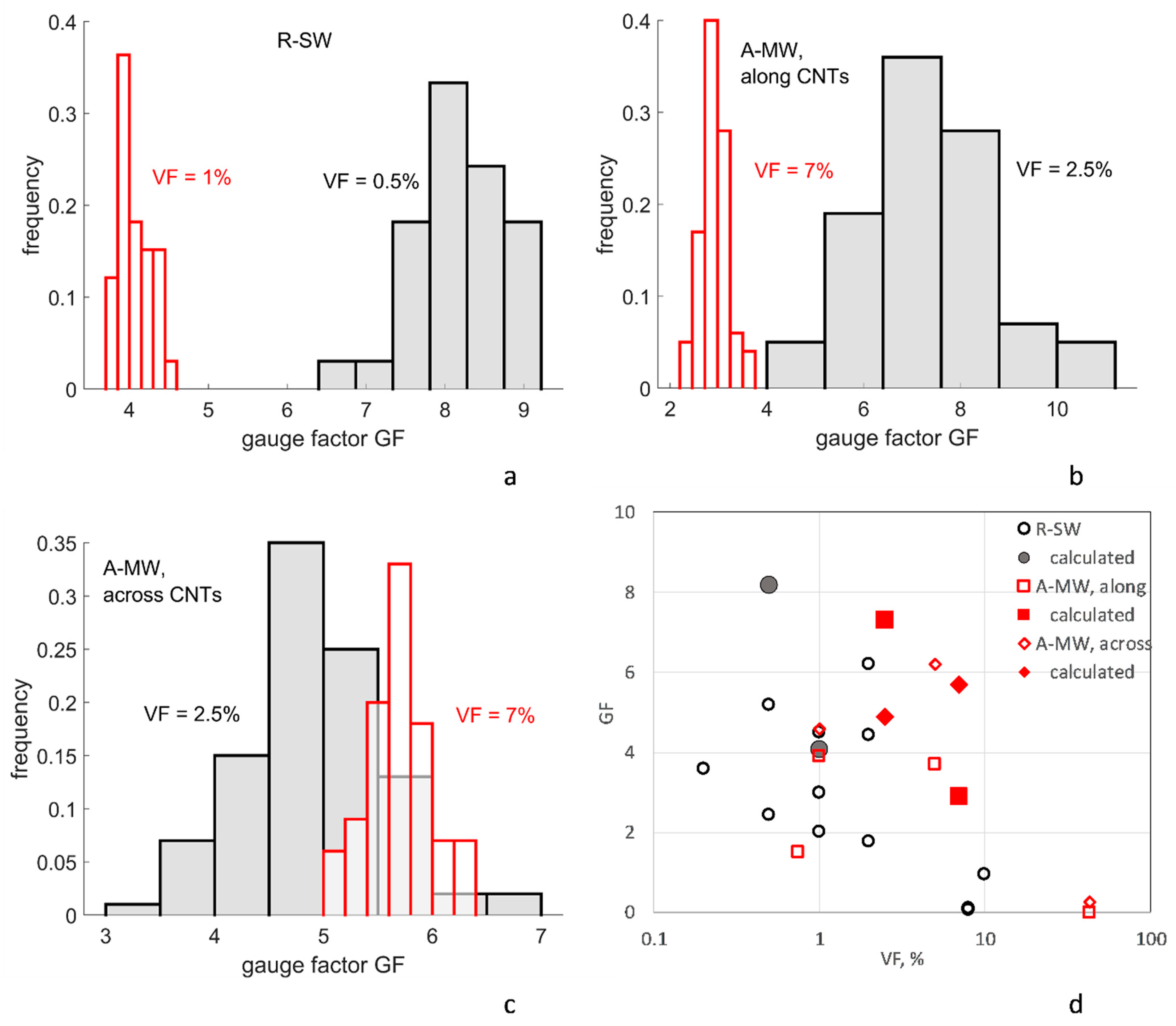
4.4.1. Deformation Sensitivity at the Reference Point of the Numerical Plan

Table 4 and Figure 9 present the results of calculation of the gauge factors GF for R-SW and A-MW configurations at the reference point of the plan for numerical experiments, with uniaxial tension strain ε = 0.01. For A-MW, two cases are considered: deformation along and across aligned CNTs. In all cases, the direction of applied voltage coincides with the direction of the applied deformation (piezoresistivity response is calculated in the direction of the deformation).
The calculated gauge factor values with parameters at the reference point are within the range of the experimentally observed GFs [65,74,75], as illustrated in Figure 9d. In contrast to dilatational loading (6), dependencies GF(VF) appear. The calculated trend GF(VF) is decreasing both for R-SW and A-MW (deformation along CNTs), which also corresponds to the literature data [65,76].
For A-MW deformation across CNTs, we observe anomalous behavior when the increase in VF does not lead to significant change in GF (the distributions of GFs overlap for VFs 2.5% and 7%). Calculations show that in this case, contrary to R-SW and A-MW deformed along CNTs, the relative change of the tunneling distances ds = (s’ − s)/s is distributed in a narrow range, ds < 1 (s’ is the tunneling distance after the deformation, s is the distance in the undeformed configuration). This is not far from a dilatational deformation, described by Equation (6), for which the change of conductivity is independent of VF. For all other cases (R-SW and A-MW along CNTs), the distributions of ds are much wider, with ds up to 100.
The calculated GF values show low scatter, with the coefficient of variation of a few percent, similar to the homogenized conductivity values (Table 3 and Figure 5). An exception is A-MW, Vf = 2.5% case, where the GF distribution for both cases along/across CNTs is wide. It is probably a result of a comparatively low number of inter-CNT contacts in this case (see Figure 3a); hence, there is a possibility for large variations of a percolating network. However, the general tendency is clear: the denser the percolation network is, and, thereby, the farther we are from the percolation threshold as a point of a phase transition, the less fluctuating behavior we observe. This tendency is related to systems with phase transitions: the closer the critical point (percolation threshold in this case) is, the more fluctuating behavior of a system becomes [92]. The decrease of the coefficient of variation for the gauge factor with the increase of the CNT volume fraction was also predicted in [33] for the aligned CNT case.

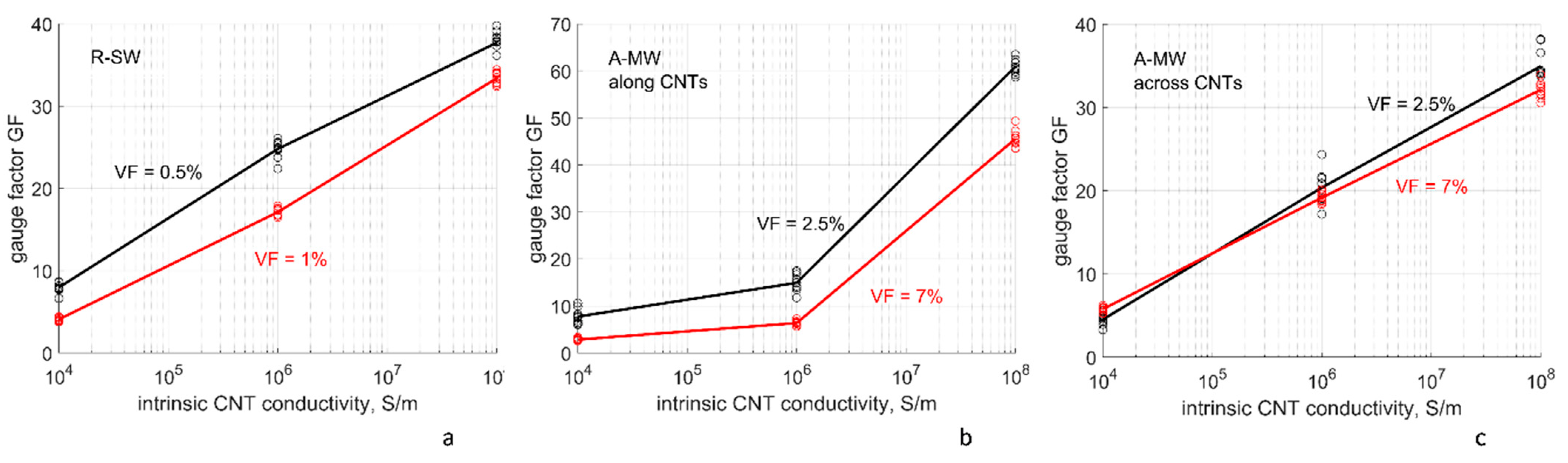
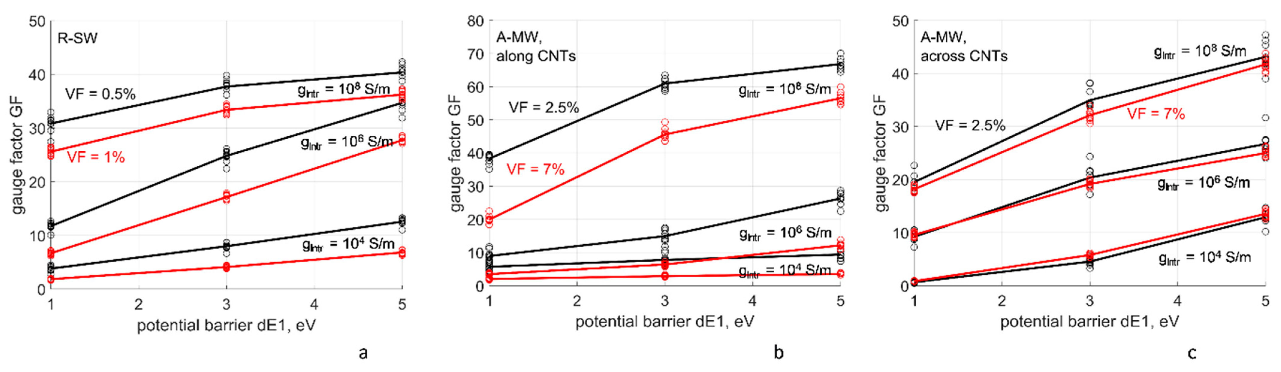
4.4.2. Dependency of Gauge Factors on Intrinsic CNT Conductivity and Tunneling Resistance

Figure 10 and Figure 11 show dependency of the gauge factors GF on the assumed parameters: the intrinsic conductivity of CNTs and potential barrier ΔE1 for the tunneling conductivity. GF grows both with the increase of gintr and with the increase of ΔE1. The dependency on the intrinsic CNT conductivity (Figure 10) can be explained by the fact that with the increase in gintr the homogenized resistivity is more strongly determined by the tunneling resistances, sensitive to deformation and, thereby, providing higher GFs. The second dependency, on the value of the potential barrier (Figure 11), is explained by the fact that tunneling resistances, determining the piezoresistive GF, increase exponentially with the increase in the square root of ΔE1. The higher ΔE1, the steeper the slope of this dependence is, providing higher GFs. In contrast to the dependency G(gintrE1), at low gintr = 104 S/m the change of ΔE1 in the range 1–5 eV changes GF by a factor 2–5 both for R-SW and A-MW, along and across CNTs. For G(104 S/m, ΔE1), this factor was 1.1–1.2 (Figure 8).
It is interesting to note that GF values for R-SW and A-MW across CNTs are quite close one to another (within ~25% difference), even in spite of the difference in VF.
Influence of the uncertainty of the input parameters on GF, calculated with the nodal analysis of CNT networks, can be characterized as follows:
-
For the same ΔE1, a change of GF is approximately proportional to a change of log(gintr);
-
For the same gintr, a change of GF is approximately proportional to a change of ΔE1.

5. Conclusions

We have conducted numerical experiments to quantify the uncertainty of the nodal analysis results for modelling of homogenized electrical conductivity tensor and deformation gauge factor for two types of CNT-based nanocomposites: randomly dispersed SWCNTs and aligned MWCNTs in a polymer matrix. The uncertainty is caused by the uncertain choice of the input parameters for analysis: the intrinsic conductivity of CNTs gintr and potential barrier ΔE1 for the tunneling resistance. The volume fraction (VF) of CNTs was chosen above the percolation threshold for all cases (0.5% and 1% for R-SW; 2.5% and 7% for A-MW).
The results of numerical experiments can be summarized as follows:
  • The scatter of the homogenized conductivity and gauge factor, caused by the randomness of a CNT assembly, is limited to few percent of coefficient of variation (CV) and is much smaller that the variations which may be caused by the difference in assumed values of the input parameters.
  • The influence of the assumed intrinsic conductivity on the homogenized conductivity and gauge factor is strong. For the intrinsic conductivity range 103–106 S/m, the dependency G(gintr) is nearly linear (to the power-law dependence with the exponent being close but below unity). For higher gintr values, its growth is asymptotically limited by the conductivity corresponding to the case of infinite intrinsic conductivity of CNTs. The assumption of infinite CNT intrinsic conductivity may bring unrealistically high simulated values for the homogenized conductivity.
  • The choice of the CNT intrinsic conductivity ~104 S/m brings the simulated homogenized conductivity and gauge factor within one order of magnitude closeness to the experimentally measured values; a better choice asks for tuning of this parameter.
  • The influence of the assumed potential barrier ΔE1 of the tunneling resistance on the homogenized conductivity is relatively weak for gintr ~ 104–106 S/m (limited to tens of percent variation for ΔE1 in the range 1–5 eV). The influence of ΔE1 becomes stronger if there are reasons to assume higher CNT intrinsic conductivity values.
  • The influence of both gintr and ΔE1 on the simulated gauge factor is strong, about one order of magnitude span for the studied range of the input parameters.
Strong dependencies of the homogenization results on the input parameters stress the necessity to evaluate a possible range of particular simulation results on the parameter choice. The findings may affect methods for optimization of nanocomposites morphology, highlighting the need to use fuzzy target functions.

Author Contributions

Conceptualization, S.V.L. and S.G.A.; Data curation, S.V.L.; Formal analysis, S.V.L. and N.A.G.; Funding acquisition, S.G.A.; Investigation, S.V.L. and S.G.A.; Methodology, S.V.L. and S.G.A.; Project administration, S.G.A.; Validation, S.V.L.; Visualization, S.V.L.; Writing—original draft, S.V.L.; Writing—review & editing, S.V.L., N.A.G. and S.G.A. All authors have read and agreed to the published version of the manuscript.

Funding

The research was funded by Skoltech NGP Program “Multifunctional Fusion: Life-cycle enhancements via data-driven nanoengineering of advanced composite structures”.

Institutional Review Board Statement

Not applicable.

Informed Consent Statement

Not applicable.

Data Availability Statement

The raw/processed data required to reproduce these findings cannot be shared at this time as the data also forms part of an ongoing study.

Acknowledgments

The authors are grateful to Keith Stevenson (Skoltech) for support of the work and constructive discussions of the manuscript.

Conflicts of Interest

The authors declare no conflict of interest.

Appendix A. Homogenization of Anisotropic Conductivity

A periodic RVE is a volume a 1 × a 2 × a 3 , with vectors of periodicity (translational symmetry) a k = a k e k   ( n o   s u m m a t i o n ) . To calculate the effective anisotropic conductivity of the medium, the RVE is placed in an average electric field E. The potential difference on face k of the volume will be
( Δ U ) k = E · a k
Ohm’s law in anisotropic medium can be written as
j = g E
where j is current density vector, [j] = A/m2, E is electrical field vector, [E] = V/m, and g is conductivity tensor, [g] = S/m. To find all components of the conductivity tensor, three cases of electrical field are considered, n = 1,2,3:
E k n = E 0 δ k n
where E0 is the scale of field, [E0] = V/m, and δ k n is Kronecker’s delta.
For these cases
( Δ U ) k n = E 0 δ n k a k   ( n o   s u m m a t i o n )
If I k n are currents through face k of the volume for case n, then the current density vector components are j k n = I k n A k , where Ak is the area of face k.
Then j k n = g k l E l n = E 0 g k l δ l n = E 0 g k n = E 0 g n k and
g n k = 1 E 0 j k n = 1 E 0 I k n A k
Currents I k n are calculated using nodal analysis.

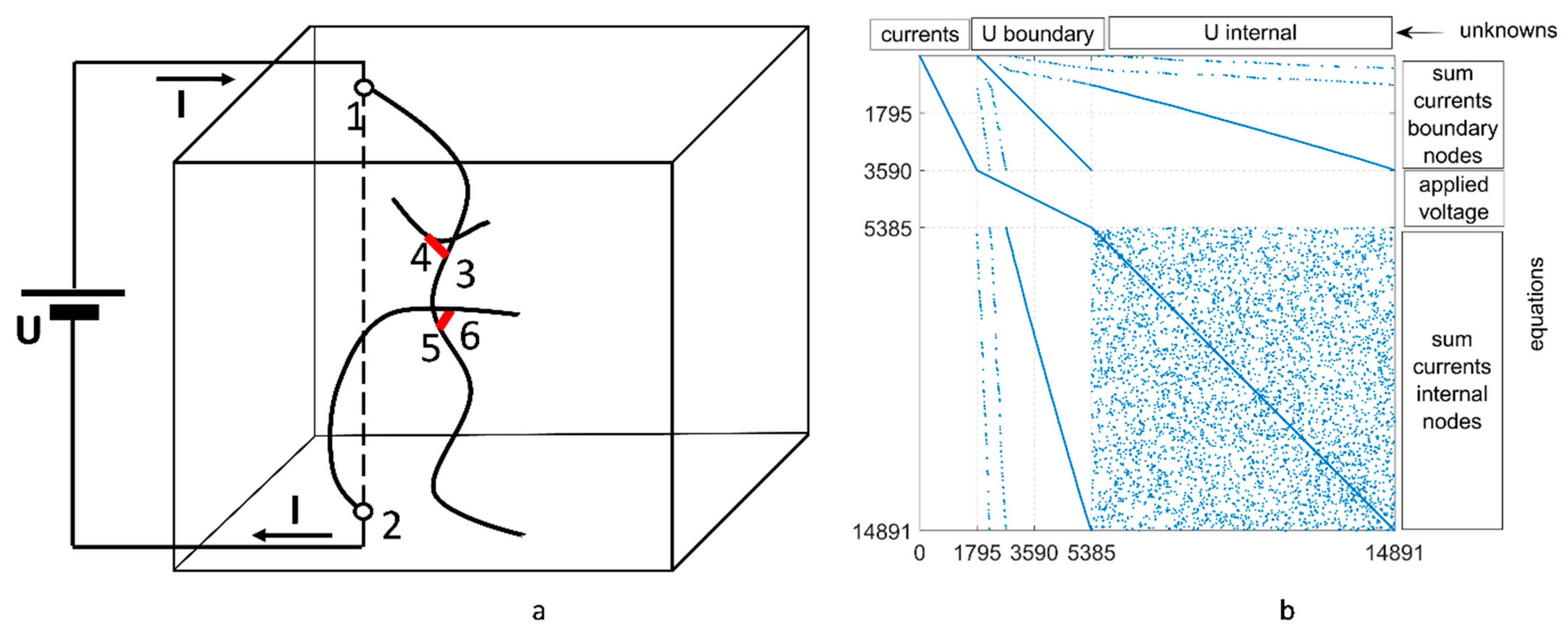
Appendix B. Nodal Analysis

For calculation of the homogenized conductivity of an RVE (see the synopsis of the homogenization process in Appendix A), the geometric network of a CNT assembly is transformed into a set of nodes connected with electrical resistances/conductances as illustrated in Figure A1. First, all contact points between the CNTs are found: two CNTs are in contact if their surfaces are closer than 1.4 nm. Then, a set of nodes of the electric circuit is defined. The set includes boundary nodes, which correspond to intersections of CNTs with the RVE faces (nodes 1 and 2 in Figure A1a); external voltage is applied to these nodes. The set also includes internal node pairs: each inter-CNT contact creates two nods, one on one CNT in contact, another on another CNT (node pairs 3,4 and 5,6 in Figure A1a).
Figure A1. Nodal analysis: (a) node pairs at contacts between CNTs, and 4, 5, and 6, boundary nodes, 1 and 2, and currents with the applied voltage; (b) the structure of the matrix of Kirchhoff’s Equations (corresponds to the A-MW case shown in Figure 2c).
Polymers 14 04794 g0a1
After the nodes are defined, a linear system of equations (“Kirchhoff’s Equations”) for nodal analysis is created, following [93]. The unknowns in these equations are currents in boundary nodes Ib, b = 1,…,Nb/2, where Nb is the number of boundary nodes on all pairs of faces, Ub for b = 1,…,Nb are electrical potentials at the boundary, and Ui, i = 1,…,Ni are electric potentials at the internal nodes. The unknowns are organized in vector X = [ I b U b U i ] T . For the case shown in Figure A1b, Nb = 3590 and Ni = 14,891 − 5385 = 9506.
The following equations form Kirchhoff’s system:
  • Nb equations for sum of currents at boundary nodes. For the nodes shown in Figure A1a,
    I + G 13 C N T ( U 3 U 1 ) = 0 I + G 25 C N T ( U 5 U 2 ) = 0
    where G p q C N T is intrinsic conductance of a CNT section between nodes p and q, calculated with Equation (1). The currents in these two equations are equal because of the periodicity of boundary conditions.
  • Nb/2 equations expressing periodic boundary conditions of the applied electrical field. For the nodes shown in Figure A1a
    U 2 U 1 = U = ( Δ U ) k n
    where ( Δ U ) k n is the potential difference for the applied voltage, Equation (A4).
  • Ni equations for the sum of currents at internal nodes. For the nodes shown in Figure A1a,
    G 13 C N T ( U 1 U 3 ) + G 53 C N T ( U 5 U 3 ) + G 43 t u n n ( U 4 U 3 ) = 0
    where G p q t u n n is tunneling conductance of a CNT between nodes p and q, calculated with Equation (2).
In total, there are Ni + 3Nb/2 equations for the same number of unknowns. The structure of the matrix K of Kirchhoff’s linear system KX = RHS is shown in Figure A1b. The system is large, and matrix K is represented as a sparse matrix in Matlab. Matrix K is singular, but Matlab function mldivide, or X = K\RHS, in most cases solves the system successfully. If it fails (returning some of the X components as NaN), the potential of one of the boundary nodes can be put to zero; after this, the operation X = K\RHS returns correct values.
After Kirchhoff’s system is solved, the full current I k n (see Equation (A5)) can be calculated as the sum of currents at the boundary nodes on face k, and the homogenized conductivity components gnk are calculated with Equation (A5).
A similar procedure is used for the case when the intrinsic conductivity of CNTs is assumed to be infinite. In this case, each CNT is treated as a node of the nodal analysis, which has an unknown potential; these nodes are connected with tunneling conductances. The sum of currents in Kirchhoff’s Equations in this case is the sum of currents in the connectors plus boundary currents in case the CNT in question crosses the RVE boundary.

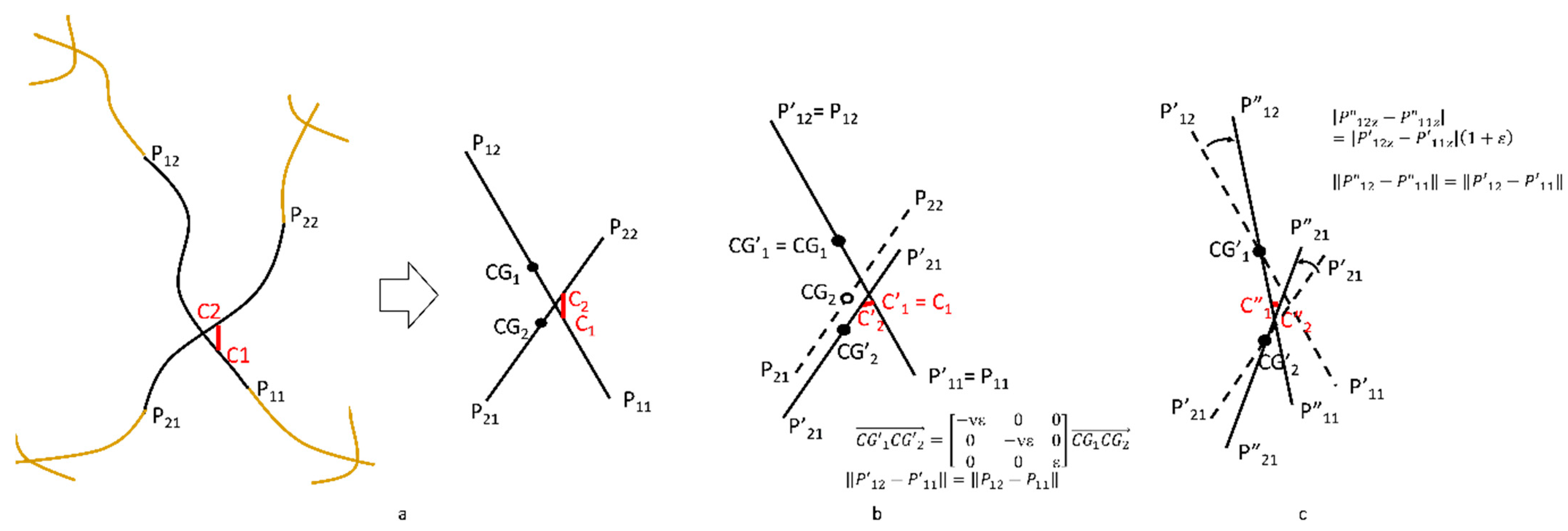
Appendix C. Change of Tunneling Contact Distances

Consider uniaxial tension of a nanocomposite, with applied deformation ε. In an R-SW case, the direction of the tension is irrelevant as the material is isotropic, and the Z-direction is chosen. In an A-MW case, the modelling is performed for tension along and across the CNT Z-direction. Value 0.3 is assumed for Poisson’s ratio of the nanocomposite [94]. Calculations of the distances of tunneling CNT contacts proceed as follows (see schematics in Figure A2, the case of uniaxial deformation in Z direction is chosen):
  • Contact C between two CNTs comprises two contact points C1 and C2 on the centrelines of these CNTs.
  • The change of a tunnelling distance in contact C between two CNTs is defined by deformation of a “deformation element” (Figure A2a), which comprises sections (P11, P12) and (P21, P22) of the CNTs with length one-half of the inter-contact CNT lengths between subsequent contacts on both sides from contact C on each of the CNTs.
  • The deformation element is approximated by two straight lines (Figure A2b), with contact points belonging to these lines, lengths of the lines equal to the lengths of CNT sections ||P11, P12|| and ||P21, P22||. The orientation of the lines is the same as of vectors P 11 , P 12 and P 21 , P 22 . The positions of contact points on the lines are the same as on CNT sections in terms of distance from contact points to the ends of sections.
  • Average deformation state of all deformation elements is the same and is defined by the applied deformation:
    ε 11 = ν ε ,   ε 22 = ν ε ,   ε 33 = ε
This is the assumption based on the fact that CNT lengths are much longer than the size of deformation elements resulting in transfer of global deformation value to local strain state. Moreover, we rely on ensemble averaging hiding rare cases deviating from the average. Losing the accuracy of 3D finite element simulations by replacing them with schematic representation, we gain computational effectiveness. The reader is referred to [78] for details of validation of the piezoresistivity model against finite elements calculations.
5.
Conformal deformation of CNTs in the deformation element has two components:
  • Displacements of the centres of gravity (CG) of the CNT sections in the element according to deformation Equation (A9), the section length is not changed, see Figure A2b, and
  • Rotation of the CNT sections around the displaced centres of gravity (CG’); the rotation increases the Z-distance between the ends of each CNT section by a factor (1 + ε) and preserves the section length, see Figure A2c
6.
The new tunnelling distance is the distance defined by the new positions of contact points C″1 and C″2, which result from the conformal deformation of the CNTs.
Figure A2. (a) A deformation element and its representation by two straight lines; (b) displacement of the centers of gravity; (c) rotation of straight sections.
Polymers 14 04794 g0a2

References

  1. Kirkpatrick, S. Percolation and Conduction. Rev. Mod. Phys. 1973, 45, 574–588. [Google Scholar] [CrossRef]
  2. Grujicic, M.; Cao, G.; Roy, W.N. A computational analysis of the percolation threshold and the electrical conductivity of carbon nanotubes filled polymeric materials. J. Mater. Sci. 2004, 39, 4441–4449. [Google Scholar] [CrossRef]
  3. Dalmas, F.; Dendievel, R.; Chazeau, L.; Cavaillé, J.Y.; Gauthier, C. Carbon nanotube-filled polymer composites. Numerical simulation of electrical conductivity in three-dimensional entangled fibrous networks. Acta Mater. 2006, 54, 2923–2931. [Google Scholar] [CrossRef]
  4. Hu, N.; Masuda, Z.; Yan, C.; Yamamoto, G.; Fukunaga, H.; Hashida, T. The electrical properties of polymer nanocomposites with carbon nanotube fillers. Nanotechnology 2008, 19, 215701. [Google Scholar] [CrossRef] [PubMed] [Green Version]
  5. Lu, W.B.; Chou, T.W.; Thostenson, E.T. A three-dimensional model of electrical percolation thresholds in carbon nanotube-based composites. Appl. Phys. Lett. 2010, 96, 223106. [Google Scholar] [CrossRef]
  6. Bao, W.S.; Meguid, S.A.; Zhu, Z.H.; Weng, G.J. Tunneling resistance and its effect on the electrical conductivity of carbon nanotube nanocomposites. J. Appl. Phys. 2012, 111, 093726. [Google Scholar] [CrossRef]
  7. Bao, W.S.; Meguid, S.A.; Zhu, Z.H.; Pan, Y.; Weng, G.J. Effect of carbon nanotube geometry upon tunneling assisted electrical network in nanocomposites. J. Appl. Phys. 2013, 113, 234313. [Google Scholar] [CrossRef]
  8. Gong, S.; Zhu, Z.H.; Haddad, E.I. Modeling electrical conductivity of nanocomposites by considering carbon nanotube deformation at nanotube junctions. J. Appl. Phys. 2013, 114, 074303. [Google Scholar] [CrossRef]
  9. Fang, W.; Jang, H.W.; Leung, S.N. Evaluation and modelling of electrically conductive polymer nanocomposites with carbon nanotube networks. Compos. Part B Eng. 2015, 83, 184–193. [Google Scholar] [CrossRef]
  10. Kulakov, V.; Aniskevich, A.; Ivanov, S.; Poltimae, T.; Starkova, O. Effective electrical conductivity of carbon nanotube–epoxy nanocomposites. J. Compos. Mater. 2016, 51, 2979–2988. [Google Scholar] [CrossRef]
  11. Bartels, J.; Kuhn, E.; Jürgens, J.-P.; Ploshikhin, V. Mesoscopic simulation of the electrical conductivity of carbon nanotube reinforced polymers regarding atomistic results. J. Compos. Mater. 2017, 52, 331–339. [Google Scholar] [CrossRef]
  12. Lubineau, G.; Mora, A.; Han, F.; Odeh, I.N.; Yaldiz, R. A morphological investigation of conductive networks in polymers loaded with carbon nanotubes. Comput. Mater. Sci. 2017, 130, 21–38. [Google Scholar] [CrossRef]
  13. Bartels, J.; Jurgens, J.-P.; Kuhn, E.; Ploshikhin, V. Effects of curvature and alignment of carbon nanotubes on the electrical conductivity of carbon nanotube-reinforced polymers investigated by mesoscopic simulations. J. Compos. Mater. 2019, 53, 1033–1047. [Google Scholar] [CrossRef]
  14. Haghgoo, M.; Ansari, R.; Hassanzadeh-Aghdam, M.K.; Nankali, M. Analytical formulation for electrical conductivity and percolation threshold of epoxy multiscale nanocomposites reinforced with chopped carbon fibers and wavy carbon nanotubes considering tunneling resistivity. Compos. Part A Appl. Sci. Manuf. 2019, 126, 105616. [Google Scholar] [CrossRef]
  15. Haghgoo, M.; Ansari, R.; Hassanzadeh-Aghdam, M.K. Prediction of electrical conductivity of carbon fiber-carbon nanotube-reinforced polymer hybrid composites. Compos. Part B Eng. 2019, 167, 728–735. [Google Scholar] [CrossRef]
  16. Tarlton, T.; Brown, J.; Beach, B.; Derosa, P.A. A stochastic approach towards a predictive model on charge transport properties in carbon nanotube composites. Compos. Part B Eng. 2016, 100, 56–67. [Google Scholar] [CrossRef]
  17. Seidel, G.D.; Lagoudas, D.C. A micromechanics model for the electrical conductivity of nanotube-polymer nanocomposites. J. Compos. Mater. 2009, 43, 917–941. [Google Scholar] [CrossRef]
  18. Feng, C.; Jiang, L. Micromechanics modeling of the electrical conductivity of carbon nanotube (CNT)–polymer nanocomposites. Compos. Part A Appl. Sci. Manuf. 2013, 47, 143–149. [Google Scholar] [CrossRef]
  19. Ivanov, S.G.; Aniskevich, A.; Kulakov, V. Simplified calculation of the electrical conductivity of composites with carbon nanotubes. Mech. Compos. Mater. 2018, 54, 61–70. [Google Scholar] [CrossRef]
  20. Hwang, M.-Y.; Kang, L.-H. CNT network modeling and simulation of the electrical properties of CNT/PNN-PZT/epoxy paint sensor. J. Mech. Sci. Technol. 2017, 31, 3787–3791. [Google Scholar] [CrossRef]
  21. Naghashpour, A.; Van Hoa, S. Requirements of amount of carbon nanotubes for damage detection in large polymer composite structures. Polym. Test. 2017, 63, 407–416. [Google Scholar] [CrossRef]
  22. Matos, M.A.S.; Tagarielli, V.L.; Baiz-Villafranca, P.M.; Pinho, S.T. Predictions of the electro-mechanical response of conductive CNT-polymer composites. J. Mech. Phys. Solids 2018, 114, 84–96. [Google Scholar] [CrossRef]
  23. Alian, A.R.; Meguid, S.A. Multiscale modeling of the coupled electromechanical behavior of multifunctional nanocomposites. Compos. Struct. 2019, 208, 826–835. [Google Scholar] [CrossRef]
  24. Lebedev, O.V.; Trofimov, A.; Abaimov, S.G.; Ozerin, A.N. Modeling of an effect of uniaxial deformation on electrical conductance of polypropylene-based composites filled with agglomerated nanoparticles. Int. J. Eng. Sci. 2019, 144, 103132. [Google Scholar] [CrossRef]
  25. Tanabi, H.; Erdal, M. Effect of CNTs dispersion on electrical, mechanical and strain sensing properties of CNT/epoxy nanocomposites. Results Phys. 2019, 12, 486–503. [Google Scholar] [CrossRef]
  26. Lebedev, O.V.; Abaimov, S.G.; Ozerin, A.N. Modeling the effect of uniaxial deformation on electrical conductivity for composite materials with extreme filler segregation. J. Compos. Mater. 2020, 54, 299–309. [Google Scholar] [CrossRef]
  27. Lebedev, O.V.; Ozerin, A.N.; Abaimov, S.G. Multiscale numerical modeling for prediction of piezoresistive effect for polymer composites with a highly segregated structure. Nanomaterials 2021, 11, 162. [Google Scholar] [CrossRef]
  28. Liu, Q.; Lomov, S.V.; Gorbatikh, L. Enhancing strength and toughness of hierarchical composites through optimization of position and orientation of nanotubes: A computational study. J. Compos. Sci. 2020, 4, 34. [Google Scholar] [CrossRef] [Green Version]
  29. Matos, M.A.S.; Tagarielli, V.L.; Pinho, S.T. On the electrical conductivity of composites with a polymeric matrix and a non-uniform concentration of carbon nanotubes. Compos. Sci. Technol. 2020, 188, 108003. [Google Scholar] [CrossRef]
  30. Matos, M.A.S.; Pinho, S.T.; Tagarielli, V.L. Application of machine learning to predict the multiaxial strain-sensing response of CNT-polymer composites. Carbon 2019, 146, 265–275. [Google Scholar] [CrossRef]
  31. Liu, Q.; Lomov, S.V.; Gorbatikh, L. Spatial distribution and orientation of nanotubes for suppression of stress concentrations optimized using genetic algorithm and finite element analysis. Mater. Des. 2018, 158, 136–146. [Google Scholar] [CrossRef]
  32. Manta, A.; Tserpes, K.I. Numerical computation of electrical conductivity of carbon nanotube-filled polymers. Compos. Part B Eng. 2016, 100, 240–246. [Google Scholar] [CrossRef]
  33. Talamadupula, K.K.; Seidel, G.D. Statistical analysis of effective electro-mechanical properties and percolation behavior of aligned carbon nanotube/polymer nanocomposites via computational micromechanics. Comput. Mater. Sci. 2021, 197, 110616. [Google Scholar] [CrossRef]
  34. Naeemi, A.; Meindl, J.D. Performance modeling for carbon nanotube interconnects. In Carbon Nanotube Electronics; Kong, J., Javey, A., Eds.; Springer: Boston, MA, USA, 2009; pp. 163–190. [Google Scholar] [CrossRef]
  35. Lee, D.H.; Lee, J.K. Initial compressional behaviour of fibre assembly. In Objective Measurement: Applications to Product Design and Process Control; Kawabata, S., Postle, R., Niwa, M., Eds.; The Textile Machinery Society of Japan: Osaka, Japan, 1985; pp. 613–622. [Google Scholar]
  36. Lomov, S.V.; Gorbatikh, L.; Verpoest, I. A model for the compression of a random assembly of carbon nanotubes. Carbon 2011, 49, 2079–2091. [Google Scholar] [CrossRef]
  37. Frank, S.; Poncharal, P.; Wang, Z.L.; De Heer, W.A. Carbon nanotube quantum resistors. Science 1998, 280, 1744–1746. [Google Scholar] [CrossRef] [Green Version]
  38. Poncharal, P.; Berger, C.; Yi, Y.; Wang, Z.L.; de Heer, W.A. Room temperature ballistic conduction in carbon nanotubes. J. Phys. Chem. B 2002, 106, 12104–12118. [Google Scholar] [CrossRef] [Green Version]
  39. Poncharal, P.; Wang, Z.L.; Ugarte, D.; de Heer, W.A. Electrostatic deflections and electromechanical resonances of carbon nanotubes. Science 1999, 283, 1513–1516. [Google Scholar] [CrossRef] [Green Version]
  40. Kobylko, M. Ballistic- and quantum-conductor carbon nanotubes: The limits of the liquid-metal contact method. Phys. Rev. B 2014, 90, 195432. [Google Scholar] [CrossRef]
  41. Kobylko, M.; Kociak, M.; Sato, Y.; Urita, K.; Bonnot, A.M.; Kasumov, A.; Kasumov, Y.; Suenaga, K.; Colliex, C. Ballistic- and quantum-conductor carbon nanotubes: A reference experiment put to the test. Phys. Rev. B 2014, 90, 195431. [Google Scholar] [CrossRef]
  42. Sammalkorpi, M.; Krasheninnikov, A.; Kuronen, A.; Nordlund, K.; Kaski, K. Mechanical properties of carbon nanotubes with vacancies and related defects. Phys. Rev. B 2004, 70, 1–8. [Google Scholar] [CrossRef] [Green Version]
  43. Zeng, H.; Zhao, J.; Hu, H.F.; Leburton, J.P. Atomic vacancy defects in the electronic properties of semi-metallic carbon nanotubes. J. Appl. Phys. 2011, 109, 083716. [Google Scholar] [CrossRef]
  44. Chiodarelli, N.; Masahito, S.; Kashiwagi, Y.; Li, Y.L.; Arstila, K.; Richard, O.; Cott, D.J.; Heyns, M.; De Gendt, S.; Groeseneken, G.; et al. Measuring the electrical resistivity and contact resistance of vertical carbon nanotube bundles for application as interconnects. Nanotechnology 2011, 22, 085302. [Google Scholar] [CrossRef] [PubMed]
  45. Chiodarelli, N.; Richard, O.; Bender, H.; Heyns, M.; De Gendt, S.; Groeseneken, G.; Vereecken, P.M. Correlation between number of walls and diameter in multiwall carbon nanotubes grown by chemical vapor deposition. Carbon 2012, 50, 1748–1752. [Google Scholar] [CrossRef]
  46. Gao, B.; Chen, Y.F.; Fuhrer, M.S.; Glattli, D.C.; Bachtold, A. Four-point resistance of individual single-wall carbon nanotubes. Phys. Rev. Lett. 2005, 95, 196802. [Google Scholar] [CrossRef] [PubMed] [Green Version]
  47. Ebbesen, T.W.; Lezec, H.J.; Hiura, H.; Bennett, J.W.; Ghaemi, H.F.; Thio, T. Electrical conductivity of individual carbon nanotubes. Nature 1996, 382, 54–56. [Google Scholar] [CrossRef]
  48. Langer, L.; Bayot, V.; Grivei, E.; Issi, J.P.; Heremans, J.P.; Olk, C.H.; Stockman, L.; Van Haesendonck, C.; Bruynseraede, Y. Quantum transport in a multiwalled carbon nanotube. Phys. Rev. Lett. 1996, 76, 479–482. [Google Scholar] [CrossRef] [Green Version]
  49. Svatos, V.; Sun, W.X.; Kalousek, R.; Gablech, I.; Pekarek, J.; Neuzil, P. Single measurement determination of mechanical, electrical, and surface properties of a single carbon nanotube via force microscopy. Sens. Actuators A-Phys. 2018, 271, 217–222. [Google Scholar] [CrossRef]
  50. Ageev, O.A.; Il'in, O.I.; Rubashkina, M.V.; Smirnov, V.A.; Fedotov, A.A.; Tsukanova, O.G. Determination of the electrical resistivity of vertically aligned carbon nanotubes by scanning probe microscopy. Tech. Phys. 2015, 60, 1044–1050. [Google Scholar] [CrossRef]
  51. Nanocyl. Technical Data Sheet NC7000 tm, V08. Available online: https://www.nanocyl.com/product/nc7000/attachment/technical-data-sheet-nc7000-v08/ (accessed on 4 April 2021).
  52. Gau, C.; Kuo, C.Y.; Ko, H.S. Electron tunneling in carbon nanotube composites. Nanotechnology 2009, 20, 395705. [Google Scholar] [CrossRef]
  53. Eken, A.E.; Tozzi, E.J.; Klingenberg, D.J.; Bauhofer, W. A simulation study on the combined effects of nanotube shape and shear flow on the electrical percolation thresholds of carbon nanotube/polymer composites. J. Appl. Phys. 2011, 109, 084342. [Google Scholar] [CrossRef]
  54. Xu, S.; Rezvanian, O.; Peters, K.; Zikry, M.A. Tunneling effects and electrical conductivity of cnt polymer composites. MRS Proc. 2011, 1304, 906–912. [Google Scholar] [CrossRef]
  55. Safdari, M.; Al-Haik, M. Electrical conductivity of synergistically hybridized nanocomposites based on graphite nanoplatelets and carbon nanotubes. Nanotechnology 2012, 23, 405202. [Google Scholar] [CrossRef] [PubMed]
  56. Di Ventra, M. Electrical Transport in Nanoscale Systems; Cambridge University Press: Cambridge, UK, 2008. [Google Scholar]
  57. Simmons, J.G. Generalized formula for the electric tunnel effect between similar electrodes separated by a thin insulating film. J. Appl. Phys. 1963, 34, 1793–1803, Comment: J. Appl. Phys. 2018, 123, 136101. [Google Scholar] [CrossRef] [Green Version]
  58. Penazzi, G.; Carlsson, J.M.; Diedrich, C.; Olf, G.; Pecchia, A.; Frauenheim, T. Atomistic modeling of charge transport across a carbon nanotube-polyethylene junction. J. Phys. Chem. C 2013, 117, 8020–8027. [Google Scholar] [CrossRef]
  59. Lomov, S.V.; Akhatov, I.S.; Lee, J.; Wardle, B.L.; Abaimov, S.G. Non-linearity of electrical conductivity for aligned multi-walled carbon nanotube nanocomposites: Numerical estimation of significance of influencing factors. In Proceedings of the 21st IEEE International Conference on Nanotechnology (IEEE-NANO), Montreal, QC, Canada, 28–30 July 2021; pp. 378–381. [Google Scholar]
  60. Yoon, Y.G.; Mazzoni, M.S.C.; Choi, H.J.; Ihm, J.; Louie, S.G. Structural deformation and intertube conductance of crossed carbon nanotube junctions. Phys. Rev. Lett. 2001, 86, 688–691. [Google Scholar] [CrossRef] [PubMed]
  61. Hu, N.; Karube, Y.; Yan, C.; Masuda, Z.; Fukunaga, H. Tunneling effect in a polymer/carbon nanotube nanocomposite strain sensor. Acta Mater. 2008, 56, 2929–2936. [Google Scholar] [CrossRef] [Green Version]
  62. Shiraishi, M.; Ata, M. Work function of carbon nanotubes. Carbon 2001, 39, 1913–1917. [Google Scholar] [CrossRef]
  63. Büttiker, M.; Imry, Y.; Landauer, R.; Pinhas, S. Generalized many-channel conductance formula with application to small rings. Phys. Rev. B 1985, 31, 6207–6215. [Google Scholar] [CrossRef] [Green Version]
  64. Li, H.J.; Lu, W.G.; Li, J.J.; Bai, X.D.; Gu, C.Z. Multichannel ballistic transport in multiwall carbon nanotubes. Phys. Rev. Lett. 2005, 95, 086601. [Google Scholar] [CrossRef]
  65. Butt, H.A.; Lomov, S.V.; Akhatov, I.; Abaimov, S. Self-diagnostic carbon nanocomposites manufactured from industrial epoxy masterbatches. Compos. Struct. 2021, 259, 113244. [Google Scholar] [CrossRef]
  66. Liddle, J.A. Transmission Electron Microscope Tomographic Data of Aligned Carbon Nanotubes in Epoxy at Volume Fractions of 0.44%, 2.6%, 4%, and 6.9%; National Institute of Standards and Technology: Gaithersburg, MD, USA, 2020. [CrossRef]
  67. Natarajan, B.; Lachman, N.; Lam, T.; Jacobs, D.; Long, C.; Zhao, M.; Wardle, B.L.; Sharma, R.; Liddle, J.A. The evolution of carbon nanotube network structure in unidirectional nanocomposites resolved by quantitative electron tomography. ASC Nano 2015, 9, 6050–6058. [Google Scholar] [CrossRef] [PubMed]
  68. Natarajan, B.; Stein, I.Y.; Lachman, N.; Yamamoto, N.; Jacobs, D.; Sharma, R.; Liddle, J.A.; Wardle, B. Aligned Carbon Nanotube Morphogenesis Predicts Physical Properties of their Polymer Nanocomposites. Nanoscale 2019, 11, 16327. [Google Scholar] [CrossRef] [PubMed] [Green Version]
  69. Cebeci, H.; Guzman de Villoria, R.; Hart, A.J.; Wardle, B.L. Multifunctional properties of high volume fraction aligned carbon nanotube polymer composites with controlled morphology. Compos. Sci. Technol. 2009, 69, 2649–2656. [Google Scholar] [CrossRef]
  70. Lomov, S.V.; Lee, J.; Wardle, B.L.; Gudkov, N.A.; Akhatov, I.S.; Abaimov, S.G. Computational description of the geometry of aligned carbon nanotubes in polymer nanocomposites. In Proceedings of the 36th ASC Technical VIRTUAL Conference (ASC 2021), Virtual, 19–22 September 2021; pp. 1606–1613. [Google Scholar] [CrossRef]
  71. Gudkov, N.A.; Lomov, S.V.; Akhatov, I.S.; Abaimov, S.G. Conductive CNT-polymer nanocomposites digital twins for self-diagnostic structures: Sensitivity to CNT parameters. Compos. Struct. 2022, 291, 115617. [Google Scholar] [CrossRef]
  72. Romanov, V.; Lomov, S.V.; Verpoest, I.; Gorbatikh, L. Modelling evidence of stress concentration mitigation at the micro-scale in polymer composites by the addition of carbon nanotubes. Carbon 2015, 82, 184–194. [Google Scholar] [CrossRef]
  73. Stein, I.Y.; Wardle, B.L. Mechanics of aligned carbon nanotube polymer matrix nanocomposites simulated via stochastic three-dimensional morphology. Nanotechnology 2016, 27, 035701. [Google Scholar] [CrossRef]
  74. Aviles, F.; Oliva-Aviles, A.I.; Cen-Puc, M. Piezoresistivity, strain, and damage self-sensing of polymer composites filled with carbon nanostructures. Adv. Eng. Mater. 2018, 20, 1701159. [Google Scholar] [CrossRef]
  75. Sánchez-Romate, X.F.; Artigas, J.; Jiménez-Suárez, A.; Sánchez, M.; Güemes, A.; Ureña, A. Critical parameters of carbon nanotube reinforced composites for structural health monitoring applications: Empirical results versus theoretical predictions. Compos. Sci. Technol. 2019, 171, 44–53. [Google Scholar] [CrossRef]
  76. Gong, S.; Wu, D.; Li, Y.; Jin, M.; Xiao, T.; Wang, Y.; Xiao, Z.; Zhu, Z.; Li, Z. Temperature-independent piezoresistive sensors based on carbon nanotube/polymer nanocomposite. Carbon 2018, 137, 188–195. [Google Scholar] [CrossRef]
  77. Wang, M.; Zhang, K.; Dai, X.X.; Li, Y.; Guo, J.; Liu, H.; Li, G.H.; Tan, Y.J.; Zeng, J.B.; Guo, Z.H. Enhanced electrical conductivity and piezoresistive sensing in multi-wall carbon nanotubes/polydimethylsiloxane nanocomposites via the construction of a self-segregated structure. Nanoscale 2017, 9, 11017–11026. [Google Scholar] [CrossRef]
  78. Lomov, S.V.; Lee, J.; Wardle, B.L.; Akhatov, I.; Abaimov, S. Piezoresistivity of nanocomposites: Accounting for cnt contact configuration changes. In Proceedings of the 20th European Conference on Composite Materials (ECCM-20), Lausanne, Switzerland, 26–30 June 2022. [Google Scholar]
  79. Lisunova, M.O.; Mamunya, Y.P.; Lebovka, N.I.; Melezhyk, A.V. Percolation behaviour of ultrahigh molecular weight polyethylene/multi-walled carbon nanotubes composites. Eur. Polym. J. 2007, 43, 949–958. [Google Scholar] [CrossRef]
  80. Gojny, F.H.; Wichmann, M.H.G.; Fiedler, B.; Kinloch, I.A.; Bauhofer, W.; Windle, A.H.; Schulte, K. Evaluation and identification of electrical and thermal conduction mechanisms in carbon nanotube/epoxy composites. Polymer 2006, 47, 2036–2045. [Google Scholar] [CrossRef]
  81. Moisala, A.; Li, Q.; Kinloch, I.A.; Windle, A.H. Thermal and electrical conductivity of single- and multi-walled carbon nanotube-epoxy composites. Compos. Sci. Technol. 2006, 66, 1285–1288. [Google Scholar] [CrossRef]
  82. Huang, Y.; Li, N.; Ma, Y.; Du, F.; Li, F.; He, X.; Lin, X.; Gao, H.; Chen, Y. The influence of single-walled carbon nanotube structure on the electromagnetic interference shielding efficiency of its epoxy composites. Carbon 2007, 45, 1614–1621. [Google Scholar] [CrossRef]
  83. Thess, A.; Lee, R.; Nikolaev, P.; Dai, H.; Petit, P.; Robert, J.; Xu, C.; Lee, Y.H.; Kim, S.G.; Rinzler, A.G.; et al. Crystalline ropes of metallic carbon nanotubes. Science 1996, 273, 483. [Google Scholar] [CrossRef] [Green Version]
  84. Chen, G.; Futaba, D.N.; Sakurai, S.; Yumura, M.; Hata, K. Interplay of wall number and diameter on the electrical conductivity of carbon nanotube thin films. Carbon 2014, 67, 318–325. [Google Scholar] [CrossRef]
  85. Lee, J.; Stein, I.Y.; Devoe, M.E.; Lewis, D.J.; Lachman, N.; Kessler, S.S.; Buschhorn, S.T.; Wardle, B.L. Impact of carbon nanotube length on electron transport in aligned carbon nanotube networks. Appl. Phys. Lett. 2015, 106, 053110. [Google Scholar] [CrossRef]
  86. Wang, D.; Song, P.; Liu, C.; Wu, W.; Fan, S. Highly oriented carbon nanotube papers made of aligned carbon nanotubes. Nanotechnology 2008, 19, 075609. [Google Scholar] [CrossRef]
  87. Marschewski, J.; In, J.B.; Poulikakos, D.; Grigoropoulos, C.P. Synergistic integration of Ni and vertically aligned carbon nanotubes for enhanced transport properties on flexible substrates. Carbon 2014, 68, 308–318. [Google Scholar] [CrossRef]
  88. Maffucci, A.; Micciulla, F.; Cataldo, A.E.; Miano, G.; Bellucci, S. Modeling, Fabrication, and Characterization of Large Carbon Nanotube Interconnects With Negative Temperature Coefficient of the Resistance. Ieee Trans. Compon. Packag. Manuf. Technol. 2017, 7, 485–493. [Google Scholar] [CrossRef]
  89. Oskouyi, A.B.; Sundararaj, U.; Mertiny, P. Tunneling Conductivity and Piezoresistivity of Composites Containing Randomly Dispersed Conductive Nano-Platelets. Materials 2014, 7, 2501. [Google Scholar] [CrossRef] [PubMed]
  90. Oskouyi, A.B.; Sundararaj, U.; Mertiny, P. A Numerical Model to Study the Effect of Temperature on Electrical Conductivity of Polymer-CNT Nanocomposites. In Proceedings of the ASME International Mechanical Engineering Congress and Exposition, San Diego, CA, USA, 15–21 November 2013; Volume 9. [Google Scholar]
  91. Kaiser, A.B.; Skakalova, V. Electronic conduction in polymers, carbon nanotubes and graphene. Chem. Soc. Rev. 2011, 40, 3786–3801. [Google Scholar] [CrossRef] [PubMed]
  92. Abaimov, S.G. Statistical Physics of Non-Thermal Phase Transitions: From Foundations to Applications; Springer: Berlin/Heidelberg, Germany, 2015; p. 493. [Google Scholar] [CrossRef]
  93. Chung-Wen, H.; Ruehli, A.; Brennan, P. The modified nodal approach to network analysis. IEEE Trans. Circuits Syst. 1975, 22, 504–509. [Google Scholar] [CrossRef] [Green Version]
  94. Dastgerdi, J.N.; Marquis, G.; Salimi, M. Micromechanical modeling of nanocomposites considering debonding and waviness of reinforcements. Compos. Struct. 2014, 110, 1–6. [Google Scholar] [CrossRef]
Figure 1. Uncertainty in electrical conductivity input data: (a) experimental data on intrinsic CNT conductivity, SWCNT (open symbols [46]), and MWCNT (filled symbols [44,47,48,49,50,51]); round points: experiments with single CNTs; squares: experiments with aligned CNTs; diamond: manufacturer’s datasheet; crosses: input data used in various modelling works; (b) tunneling conductance of a contact between two CNTs in function of the distance between them; results for SWCNTs and MWCNTs are calculated with Equations (2)–(4).
Polymers 14 04794 g001
Figure 2. Geometrical model: (a) parameters of a CNT segment; central paths of CNTs in (b) RVE for R-SW, VF = 1%; (c) RVE for A-MW; VF = 7%, 3D view (left) and view from the end of the Z-axis (right).
Polymers 14 04794 g002
Figure 3. Characteristics of contacts for random RVEs: (a) density of CNT contacts, points: calculated values for random RVEs (the scatter is not noticeable for R-SW), lines: prediction according to Equation (8); (b) distribution of the tunneling conductances of CNT contacts, ΔE1 = 3 eV, smin = 0.34 nm, typical RVEs for R-SW (VF = 1%) and A-MW (VF = 7%) cases; (c,d) distribution of distances along CNTs between the contacts for R-SW (c) and A-MW (d) cases; mean values are shown in the legends.
Polymers 14 04794 g003
Figure 4. Comparison between the resistance of a typical CNT segment between two contacts for two values of VF (solid lines) and the tunneling resistance in the contact for s = 0.34 nm for two values of ΔE1 (dashed lines), R-SW (a) and A-MW (b).
Polymers 14 04794 g004
Figure 5. Conductivity tensor components for R-SW, histograms of the distributions: diagonal VF = 0.5% (a); VF = 1% (b); and off-diagonal VF = 0.5% and 1% components (c); the reference point of the numerical plan: gintr = 104 S/m; ΔE1 = 3 eV; smin = 0.34 nm; sampling size ≥ 99 for all cases.
Polymers 14 04794 g005
Figure 6. Conductivity tensor components for A-MW, histograms of the distributions: VF = 2.5% (ac); and VF = 7% (df); conductivity along CNTs (a,d); across CNTs (b,e); and off-diagonal (c,f); the reference point of the numerical plan: gintr = 104 S/m; ΔE1 = 3 eV; smin = 0.34 nm; sampling size ≥ 99 for all cases.
Polymers 14 04794 g006
Figure 7. The homogenized conductivity as a function of the assumed intrinsic conductivity of CNTs, at two levels of the CNT volume fraction: (a) R-SW, diagonal components of the conductivity tensor; (b) A-MW, along CNTs; (c) A-MW, across CNTs. The dashed lines show homogenized conductivity calculated assuming infinite conductivity of CNTs. The points show conductivity values, corresponding to different RVE random realizations (sampling size ≥ 99 for all cases). ΔE1 = 3 eV, smin = 0.34 nm, the lines show mean values. The horizontal boxes show the homogenized conductivity range measured for R-SW [65] and A-MW [69] experimentally. The colors of the lines, points, and boxes correspond to CNT volume fractions, as shown on the graphs.
Polymers 14 04794 g007
Figure 8. The homogenized conductivity as function (ac) of the assumed potential barrier ΔE1 for the tunneling conductivity, with smin = 0.34 nm, and (df) of the minimal distance between CNTs, with ΔE1 = 3 eV, at three levels of the CNT intrinsic conductivity gintr and two levels of the CNT volume fraction: (a,d) R-SW, diagonal components of the conductivity tensor; (b,e) A-MW, along CNTs; (c,f) A-MW, across CNTs. The points show conductivity values corresponding to different RVE random realizations (sampling size ≥ 99 for all cases); the lines show mean values. The horizontal boxes show the homogenized conductivity range measured for R-SW [65] and A-MW [69] experimentally. The colors of the lines, points, and boxes correspond to CNT volume fractions, as shown on the graphs.
Polymers 14 04794 g008
Figure 9. The gauge factors, Equation (5), ε = 0.01, histograms of the distributions: (a) R-SW, VF = 0.5% and 1%; (b,c) A-MW, along (b) and across (c) CNTs, VF = 2.5% and 7%; (d) experimental data [65,74,75], open symbols, in comparison with the computed values (closed symbols). The reference point of the experimental plan: gintr = 104 S/m; ΔE1 = 3 eV; smin = 0.34 nm. Sampling size ≥ 99 for all cases.
Polymers 14 04794 g009
Figure 10. The gauge factors as a function of the assumed intrinsic conductivity of the CNTs, at two levels of the CNT volume fraction: (a) R-SW; (b) A-MW, along CNTs; (c) A-MW across CNTs. The points show conductivity values corresponding to different RVE random realizations; the lines show mean values; ΔE1 = 3 eV; smin = 0.34 nm.
Polymers 14 04794 g010
Figure 11. The gauge factors as functions of the assumed potential barrier ΔE1 for the tunneling conductivity, smin = 0.34 nm, at three levels of the CNT intrinsic conductivity gintr and two levels of the CNT volume fraction: (a) R-SW; (b,c) A-MW: along CNTs (b) and across CNTs (c). The points show conductivity values, corresponding to different RVE random realizations; the lines show mean values.
Polymers 14 04794 g011
Table 1. Parameters of the modelled CNT nanocomposites.
ParameterR-SWA-MW
Data source[65][66,68]
CNT outer diameter, nm1.68.0
CNT length
Distribution typeWeibullconstant
Mean length, µm2.020
Weibull modulus3.0n/a
Weibull scale, µm2.24n/a
CNT orientation
Distribution typeuniformaligned
CNT shape
Maximal curvature, 1/µm55
Maximal torsion, 1/µm55
Volume fraction variants0.5%; 1%2.5%; 7%
Table 2. Plan of numerical experiments, values in bold correspond to the reference point.
Parameter Variation TypeIntrinsic CNT Conductivity, S/MPotential Barrier ΔE1, eVMinimal CNT Distance, Nm
Varying intrinsic CNT conductivity and potential barrier for tunneling conductivity103 104 105 106
107 108
1
3
5
0.34
Varying minimal CNT distance10430.25
Table 3. Homogenized conductivity tensor components at the reference point of the numerical plan: gintr = 104 S/m, ΔE1 = 3 eV, and smin = 0.34 nm.
TypeVFDiagonal Components, S/MOff-Diagonal Components, S/M
Signed ValuesAbsolute Values
R-SW0.5%12.7 ± 0.33 (2.5%)−0.007 ± 0.2900.217 ± 0.195 (87%)
1%28.6 ± 0.55 (1.9%)0.030 ± 0.4220.334 ± 0.258 (77%)
A-MW along CNTsacross CNTs
2.5%217 ± 1.44 (0.66%)3.03 ± 0.23 (7.5%)−0.0015 ± 1.200.816 ± 0.874 (107%)
7.0%630 ± 0.86 (0.13%)13.8 ± 0.32 (2.3%)−0.140 ± 2.111.47± 1.52 (103%)
Notes: ± means standard deviation; the value in brackets gives coefficient of variation (not given for signed values of the non-diagonal components as their mean is close to zero).
Table 4. Gauge factors, Equation (5), for unidirectional tension deformation 0.01 in Z-direction, the reference point of the numerical plan: gintr = 104 S/m, ΔE1 = 3 eV, smin = 0.34 nm.
TypeVFGauge Factor GF
R-SW0.5%8.18 ± 0.57 (7.0%)
1%4.07 ± 0.21 (2.5%)
A-MW, along CNTs2.5%7.32 ± 1.34 (18.3%)
7.0%2.91 ± 0.27 (9.3%)
A-MW, across CNTs2.5%4.89 ± 0.62 (12.6%)
7.0%5.69 ± 0.28 (4.9%)
Note: ± means standard deviation; the value in brackets gives coefficient of variation.
Publisher’s Note: MDPI stays neutral with regard to jurisdictional claims in published maps and institutional affiliations.

