Article

Photoaligned Tunable Liquid Crystal Lenses with Parabolic Phase Profile

by
Svitlana P. Bielykh
1,
Liana Lucchetti
2,* and
Victor Yu. Reshetnyak
1,3
1
Theoretical Physics Department, Physics Faculty, National Taras Shevchenko University of Kyiv, Volodymyrs’ka Street 64, 01601 Kyiv, Ukraine
2
Dipartimento SIMAU, Università Politecnica delle Marche, Via Brecce Bianche, 60131 Ancona, Italy
3
Department of Physics, University of Warwick, Coventry CV4 7AL, UK
*
Author to whom correspondence should be addressed.
Crystals 2023, 13(7), 1104; https://doi.org/10.3390/cryst13071104
Submission received: 26 June 2023 / Revised: 7 July 2023 / Accepted: 11 July 2023 / Published: 15 July 2023

Abstract

:
We present a theoretical model of a cylindrical tunable liquid crystal lens based on the modulation of anchoring energy. The latter can be easily obtained using photoalignment techniques. The liquid crystal cell we propose exhibits strong anchoring at the top substrate and anchoring energy with a parabolic profile at the bottom substrate. The model describes the dependence of the focal length on the applied voltage and presents a theoretical study of the lens aberrations. The results obtained are of general relevance and can be used to optimize the performances of every type of liquid crystal lens with a parabolic profile.

1. Introduction

Conventional lenses are based on the radial shaping of materials, like glass or plastic, that exhibit a constant refractive index. These optical components typically have one fixed focal length. The standard method of varying the focal length of an imaging system is to use a certain number of lenses such that the focus position is changed by mechanically adjusting their mutual distance. This approach makes the system bulky and unsuitable for certain applications. Compact and lightweight optical systems, where the focal length can be varied without moving parts, are clearly very attractive. The fluid nature of the director field in liquid crystals (LC), combined with their high sensitivity to external stimuli, enables lenses based on liquid crystalline materials to fulfill the above requirements. The focal length of LC lenses is typically electrically tunable, and since the first report dated back to 1979 [1], several different structures have been proposed, mainly based on patterned electrodes [2,3,4,5,6,7]. In these systems, a lens-like refractive index profile is realized by pixelated electrodes with a proper distribution. LC cells with pixel-free electrodes have also been proposed [8]. The LC lens described in [8] consists of a sandwich LC planar cell with uniform ITO-coated substrates and is based on the light-induced reduction of the Fredericks threshold in LC cells doped with azo dyes [9]. Indeed, a Gaussian beam incident on an azo-dye-doped LC cell gives rise to the adsorption and desorption of dye molecules on the irradiated cell surface; the dominant effect is dependent on both light intensity and polarization [10]. Since dye doping forms charge complexes in LC [11], the light-induced adsorbed layer affects the surface charge density and, as a consequence, the effective internal voltage felt by the LC molecules. This means that the Fredericks threshold is modulated and, due to the dependence of the density of adsorbed and desorbed molecules on light intensity, the threshold electric field required to reorient the LC molecules follows a Gaussian beam profile. Therefore, the applied dc field produces a director distortion that gives rise to a lens-like refractive index distribution [8].
Despite being more than 40 years old and a large number of existing literatures, LC lenses continue to attract the interest of the scientific community due to the great number of possible applications. Some new devices, such as head-mounted displays, mobile cameras, and contact lenses, have indeed demonstrated the need for novel adaptive lenses [12], and non-conventional solutions have recently been proposed [13,14,15,16]. In addition, different driving methods for controlling LC microlens arrays to be used in switchable displays [17] and hyperspectral imaging [18] are currently being investigated. The design, fabrication, and characterization of an ultrathin, polarization-insensitive focus-tunable LC diffractive lens with a large aperture, low weight, and low operating voltage have also been proposed and used for the realization of augmented reality glasses [19].
With the aim of contributing to the recent efforts, we propose a theoretical study of LC lenses based on a parabolic profile of the anchoring energy that can easily be produced by photoalignment of proper transparent surface coatings [20,21,22,23]. Specifically, photoalignment consists of coating the LC cell substrates with a UV-curable polymer transparent to VIS light, which is then exposed to a linearly polarized UV light beam. The polarized exciting light initiates orientationally selective photoexcitation of the molecules of the aligning material, leading to their bulk and surface orientational ordering. The order induced in the aligned film and the characteristics of the LC-substrate interaction determine the orientation of the LC easy axis. The photoaligning effect occurs due to the anisotropic interaction of LC molecules with the orientationally ordered alignment polymer. Reversible LC photoalignment has also been demonstrated by the proper selection of aligning layers [24,25].
Our simulations show that the application of an external voltage V in a range of 0.7–1 V produces a tunable parabolic modulation of the LC birefringence. Both the phase delay and focal length are calculated for different values of V and the lens aberrations are estimated.
It should be noted that LC lenses with parabolic phase profiles have recently been proposed [7]. In the study, a parabolic profile was obtained using a proper electrode pattern that gave rise to a parabolic distribution of the applied voltage. Our approach, on the contrary, is based on photoalignment and does not require any electrode patterning. The advantages of photoalignment over electrode patterning are manyfold. One is related to the absence of mechanical rubbing, which is critical for many applications that require LC alignment with high microscopic uniformity and fine alignment patterning. Moreover, photoalignment allows easier alignment on relief, curved, and flexible substrates, as well as in confined volumes. Overall, strong anchoring, stable pretilt, and negligibly weak image sticking are possible with these techniques [26].

2. Modeling the LC Lens

Let us consider a nematic liquid crystal (LC) cell of thickness L and width D with spatially modulated anchoring. Specifically, we assume strong planar anchoring at the top substrate and an anchoring energy dependent on the distance from the center of the cell at the bottom substrate [27]. A sketch of the cell is shown in Figure 1. In this figure, the OZ axis passing through the cell center and perpendicular to the plane of the cell is shown together with the lens width D and the lens aperture R.
When a proper external voltage V is applied to the cell along Z, the LC director n reorients by an amount that depends on both the value of V and the value of the anchoring energy W x . As the anchoring spatially is modulated, this reorientation is also modulated, thus giving rise to a lens-like refractive index profile. The focal length of the resulting lens depends on the applied voltage and is thus electrically tunable.
We assumed an anchoring energy profile W(x) at the bottom substrate of the cell using the following formula:
W x = W 1 , 0 x D R / 2 2 W 1 W 1 x D 2 2 R 2 2 , D R / 2 x D + R / 2 W 1 , D + R / 2 x D
where D is the lens width, R is the lens aperture, and W 1 is the constant minimum anchoring energy (see Table 1). W(x) is shown in Figure 2. The value of W 1 has been chosen based on previous investigations [22,23,28].
We modeled a cylindrical lens, which simplifies the problem to the 2D case with respect to the 3D approach required for conventional spherical lenses.

3. Director Reorientation under Action of Externally Applied Voltage in the Cell with Modulated Anchoring Energy

To investigate the electro-optical properties of the proposed LC lens, one needs to determine the director reorientation angle θ x , z . It is noteworthy that we assumed the voltage induced LC reorientation to be confined in the XY plane; therefore, this is the only angle that needs to be calculated.
The director field has the form n = cos θ x , z , 0 , sin θ x , z , and the total free energy density F is calculated as follows:
F = F e l a s i c + F e l e c t r i c + F s u r f a c e ,
where
F e l a s t i c = V K 11 2 d i v n 2 + K 22 2 n c u r l n 2 + K 33 2 n × c u r l n 2 d V ,
is the elastic free energy density,
F e l e c t r i c = 1 2 V D E d V ,
represents the dielectric coupling with the external electric field, and the surface of the total free energy density is calculated as follows [29]:
F s u r f a c e = 1 2 S i S i W i d n 2 d S i ,
K i i is the LC elastic constant, D is the electric displacement vector, E is the externally applied electric field, d is the easy axis direction, and W i (i = 1,2) is the anchoring energy of the LC cell bounding substrates.
Substituting Equations (3)–(5) into Equation (2) and minimizing F , one obtains the following Euler–Lagrange equation for θ x , z :
θ x x K 11 s i n 2 θ + K 33 c o s 2 θ + θ z z K 11 c o s 2 θ + K 33 s i n 2 θ + K 33 K 11 θ z 2 θ x 2 sin θ cos θ + θ x z sin 2 θ + θ x θ z cos 2 θ + ε 0 ε α sin θ cos θ E z 2 E x 2 + E z E x cos 2 θ = 0
where ε a = ε | | ε is the LC dielectric anisotropy, i.e., the difference between the dielectric constants in the directions parallel and perpendicular to n.
Considering finite director anchoring at the bottom substrate and strong anchoring at the top substrate, the boundary conditions take the following form:
K 33 s i n 2 θ + K 11 c o s 2 θ θ z z = 0 W x sin θ 0 θ 1 cos θ 0 θ 1 = 0 , θ z = L = θ 2
Equations (6) and (7) should be accompanied by the Poisson equation for the electric field potential U , defined by the relation E = U [18]
ε ~ ε 0 U x , z = 0 ,
where ε ~ ε 0 = ε ^ ε 0 + i σ ω , with ε ~ as the permittivity tensor, ω as the AC electric field frequency, σ as the LC electric conductivity, and ε ^ as the LC dielectric tensor. In our case, the latter has the following form:
ε ^ = ε + ε a cos 2 θ 0 ε a sin θ cos θ 0 ε 0 ε a sin θ cos θ 0 ε + ε a sin 2 θ
The electric field potential U x , z obeys the following boundary conditions:
U z = 0 = 0 U z = L = V
where V is the voltage applied to the cell at z = L . In this way, one obtains the following system of equations for the director field θ x , z and for the electric field potential U x , z with the following boundary conditions:
θ x x K 11 s i n 2 θ + K 33 c o s 2 θ + θ z z K 11 c o s 2 θ + K 33 s i n 2 θ + K 33 K 11 θ z 2 θ x 2 sin θ cos θ + θ x z sin 2 θ + θ x θ z cos 2 θ + ε 0 ε α sin θ cos θ E z 2 E x 2 + E z E x cos 2 θ = 0 ε ~ ε 0 U x , z = 0 K 33 s i n 2 θ + K 11 c o s 2 θ θ z z = 0 W x sin θ 0 θ 1 cos θ 0 θ 1 = 0 θ z = L = θ 2 U z = 0 = 0   U z = L = V
The system of Equation (11) has no analytical solution. To solve this, it is necessary to perform computer calculations. The parameters we used in the calculations are shown in Table 1. The values selected for the splay, K11, and bend, K33, elastic constants are of the order of the most common thermotropic LCs [27,30]. An example of a nematic LC exhibiting similar elasticity, dielectric constants, and birefringence as those reported in Table 1 is provided by the two mixtures 1825 and 1852 described in [31,32], both exhibiting a nematic phase at room temperature.
By solving Equation (11) with numerical calculations, we obtained the reorientation angle of the director θ x , z and the electric potential U x , z at different values of the external voltage.
The electric field potentials calculated for V = 1   V and V = 0.8   V in the middle of the cell z = L/2 as a function of x are reported in Figure 3a,b, respectively. Figure 4 shows the LC director profile for different values of V and at different positions in the cell. Specifically, Figure 4a,b,e,f show θ x , z at z = L/2 as a function of x for different voltages; in Figure 4c,d, θ x , z is instead shown as a function of z at x = D/2 for V = 0.8 V (c) and V = 1 V (d). As expected, the director followed the profile of the electric field potential.

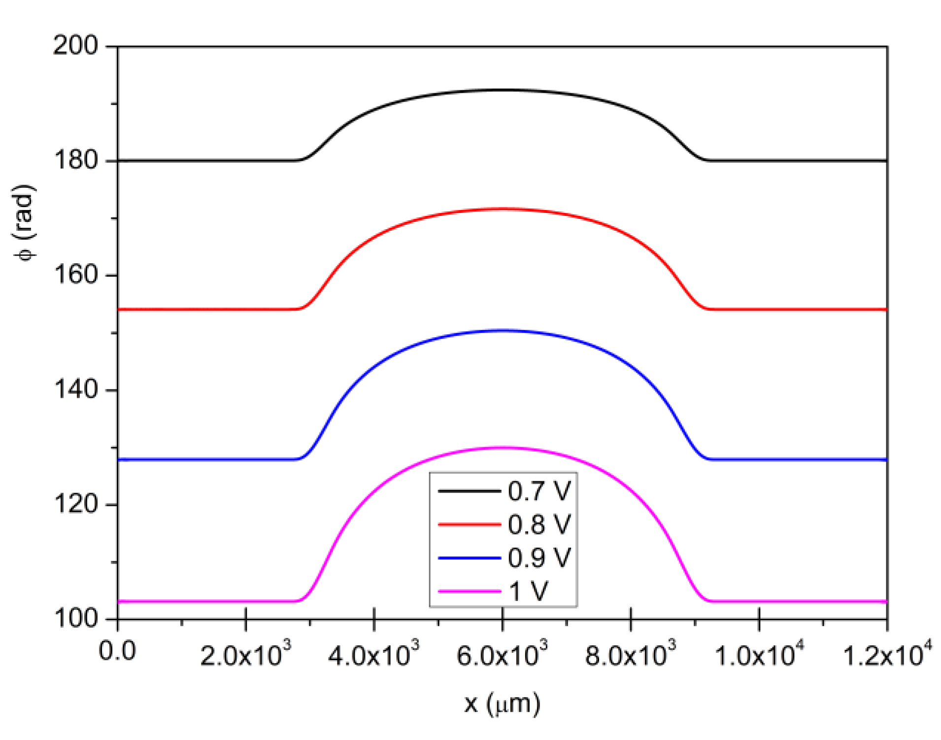
4. Light Propagation through LC Cell Subjected to Externally Applied Voltage

In the previous section, we calculated the spatial profile of the LC director subjected to an externally applied voltage. The refractive index for an extraordinary beam propagating in the LC cell is given by the following relation:
n e f f ψ = n 0 n e n e 2 cos 2 ψ + n 0 2 sin 2 ψ
where ψ is the angle between the LC director (which defines the optical axis) and the light wave vector. In our case, ψ = π 2 θ .
We treated the LC cell with a lens-like director distribution as a thin phase plate. The phase retardation ϕ experienced by a test light beam propagating through the cell is defined as
ϕ = 2 π λ 0 L n e f f θ d z
and depends on the distance x from the center of the cell. This is shown in Figure 5 for different values of the applied voltage V. This dependence determines the focusing properties of the LC lens.
To evaluate the focal length of the LC lens, we fitted the curves ϕ = ϕ (x) in Figure 5 to a parabola according to the paraxial approximation [33,34] using the following equation:
ϕ x = a k x 2 2 f ,
where a = ϕ 0 is the phase shift at the center of the LC cell, f is the focal length of the LC lens, and k is the modulus of the test beam wave vector.
The inverse of the obtained focal length is shown in Figure 6 as a function of the applied voltage V for a lens aperture of R = 1 mm. The electrical tunability of the lens focus is well represented by this curve.

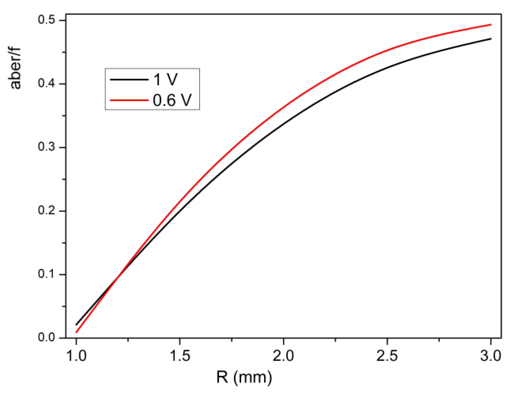
5. Aberration of LC Lens with Modulated Anchoring Energy

Optical lenses and LC lenses do not make exceptions and are not ideal optical systems. Indeed, there is always some degree of aberration introduced by the lens, which causes the image to be an imperfect replica of the object. Thus, aberration plays an important role in the formation of images; among them, spherical aberration is the most common when dealing with monochromatic light.
Figure 7 shows the definition of spherical aberration. A spherically aberrated lens does not have a well-defined focus. The distance along the optical axis between the intercept of the rays that are near the optical axis (paraxial rays, point F ) and the rays that pass through the edge of the lens (marginal rays, point F 1 ) is called the longitudinal spherical aberration (LSA, F F 1 ) [34].
Theoretically, to obtain the LSA in an LC lens, it is necessary to determine the beam trajectory in an inhomogeneous liquid crystal cell [35,36,37]. In this study, we propose a simpler and quicker approach.
In the previous section, to determine the focal length of the LC lens, we used the paraxial approximation, which holds for a beam that is as close as possible to the optical axis of the lens [33], as well as for an ideal spherical wavefront. However, as the aperture of the lens R increases, this approximation becomes increasingly less fulfilled.
In Figure 8, one can see the phase retardation (Equation (13)) compared to the one modeled using the paraxial approximation (Equation (14)) for different lens apertures R = 1 mm (a) and R = 3 mm (b), for an applied voltage V = 0.7 V. As R increases from 1 to 3 mm, the quality of the approximation worsens, indicating an imperfect lens and that aberrations must be estimated.
To estimate the LSA, we determined the location of the beam from the edge of the lens aperture. To this end, we used the paraxial approximation (14) to describe the beam wavefront near the lens aperture point. Mathematically, this means that we approximated a part of the wavefront near the lens aperture and found the approximation coefficients. Next, we found a point on the axis of this parabola, where the rays from the edge of the aperture converge. Using mathematical formulas, we projected it onto the axis of the lens. Thus, we obtained the point from where the rays came from the edge of the lens (lens aperture).
Figure 9 shows the relative longitudinal spherical aberration, defined as the ratio between the LSA and the focal length, versus the lens aperture R, for V = 0.8 V (black line) and V = 1 V (red line).
The relative longitudinal spherical aberration as a function of the applied voltage at fixed values of R (R = 1.5 mm and R = 2 mm) is shown in Figure 10a,b.
The relative LSA increased with R, as expected, and slightly decreased with increasing V, which we understand as a voltage-induced change in the phase profile. The increasing voltage makes the phase profile “more parabolic”.

6. Conclusions

We proposed a theoretical model that describes the properties of a cylindrical LC lens with a parabolic phase profile induced by spatially modulated anchoring energy. We calculated the director profile, the electric field potential in the LC cell, and the phase delay experienced by a light beam propagating through the cell. Moreover, we estimated the focal length and the longitudinal spherical aberration of the LC lens. The dependence of the focal length on the applied voltage demonstrates the electrical tunability of the modeled lens.
The observed dependence of the lens aberration on the external voltage and the lens aperture allows for optimizing the lens features to obtain the best image quality. As an example, by combining f and LSA, it is possible to look for the conditions that provide the highest optical power with the lowest aberrations. The obtained results can easily be applied to experimentally developed LC lenses. Indeed, in principle, photoalignment allows obtaining different profiles of the anchoring energy so that the phase retardation can become closer to the parabolic profile in a wide range of externally applied voltages, thus reducing the aberrations. We expect that AI or machine learning can also help determine the optimal profile of the anchoring energy.
Proper experiments will be conducted soon to validate the above predictions.

Author Contributions

Conceptualization, V.Y.R.; Methodology, V.Y.R.; Software, S.P.B.; Validation, L.L. and V.Y.R.; Formal analysis, S.P.B.; Investigation, S.P.B.; Data curation, S.P.B.; Writing – original draft, LL; Writing – review & editing, S.P.B. and L.L.; Supervision, V.Y.R. All authors have read and agreed to the published version of the manuscript.

Funding

This research received no external funding.

Data Availability Statement

All data are available upon request to the authors.

Conflicts of Interest

The authors declare no conflict of interest.

References

  1. Sato, S. Liquid-Crystal Lens-Cells with Variable Focal Length. Jpn. J. Appl. Phys. 1979, 18, 1679. [Google Scholar] [CrossRef]
  2. Riza, N.A.; DeJule, M.C. Three-terminal adaptive nematic liquid-crystal lens device. Opt. Lett. 1994, 19, 1013–1015. [Google Scholar] [CrossRef]
  3. Ren, H.; Wu, S.-T. Tunable electronic lens using a gradient polymer network liquid crystal. Appl. Phys. Lett. 2003, 82, 22–24. [Google Scholar] [CrossRef] [Green Version]
  4. Ye, M.; Yokoyama, Y.; Sato, S. Liquid crystal lens prepared utilizing patterned molecular orientations on cell walls. Appl. Phys.Lett. 2006, 89, 141112. [Google Scholar] [CrossRef]
  5. Ye, M.; Wang, B.; Sato, S. Liquid crystal lens with focus movable in focal plane. Opt. Commun. 2006, 259, 710–722. [Google Scholar] [CrossRef]
  6. Algorri, J.F.; Morawiak, P.; Bennis, N.; Zografopoulos, D.C.; Urruchi, V.; Rodríguez-Cobo, L.; Jaroszewicz, L.R.; Sánchez-Pena, J.M.; López-Higuera, J.M. Positive-negative tunable liquid crystal lenses based on a microstructured transmission line. Sci. Rep. 2020, 10, 10153. [Google Scholar] [CrossRef]
  7. Feng, W.; Liu, Z.; Liu, H.; Ye, M. Design of Tunable Liquid Crystal Lenses with a Parabolic Phase Profile. Crystals 2023, 13, 8. [Google Scholar] [CrossRef]
  8. Lucchetti, L.; Tasseva, J. Optically recorded tunable microlenses based on dye-doped liquid crystal cells. Appl. Phys. Lett. 2012, 100, 181111. [Google Scholar] [CrossRef]
  9. Lucchetti, L.; Catani, L.; Simoni, F. Light-controlled electric Freedericksz threshold in dye doped liquid crystals. J. Appl. Phys. 2014, 115, 203111. [Google Scholar] [CrossRef]
  10. Francescangeli, O.; Lucchetti, L.; Simoni, F.; Stanić, V.; Mazzulla, A. Light-induced molecular adsorption and reorientation at polyvinylcinnamate-fluorinated/liquid-crystal interface. Phys. Rev. E 2005, 71, 011702. [Google Scholar] [CrossRef]
  11. Lucchetti, L.; Gentili, M.; Simoni, F. Colossal optical nonlinearity induced by a low frequency external electric field in dye-doped liquid crystals. Opt. Express 2006, 14, 2236–2241. [Google Scholar] [CrossRef]
  12. Algorri, J.F.; Zografopoulos, D.C.; Urruchi, V.; Sánchez-Pena, J.M. Recent Advances in Adaptive Liquid Crystal Lenses. Crystals 2019, 9, 272. [Google Scholar] [CrossRef] [Green Version]
  13. Zhan, T.; Lee, Y.-H.; Tan, G.; Xiong, J.; Yin, K.; Gou, F.; Zou, J.; Zhang, N.; Zhao, D.; Yang, J.; et al. Pancharatnam–Berry optical elements for head-up and near-eye displays. Opt. Soc. Am. B 2019, 36, D52–D65. [Google Scholar] [CrossRef]
  14. Ma, Y.; Tam, A.M.W.; Gan, X.T.; Shi, L.Y.; Srivastava, A.K.; Chigrinov, V.G.; Kwok, H.-S.; Zhao, J.L. Fast switching ferroelectric liquid crystal Pancharatnam–Berry lens. Opt. Express 2019, 27, 10079–10086. [Google Scholar] [CrossRef]
  15. Jamali, A.; Bryant, D.; Zhang, Y.; Grunnet-Jepsen, A.; Bhowmik, A.; Bos, P.J. Design of a large aperture tunable refractive Fresnel liquid crystal lens. Appl. Opt. 2018, 57, B10–B19. [Google Scholar] [CrossRef]
  16. Lin, H.-Y.; Avci, N.; Hwang, S.-J. High-diffraction-efficiency Fresnel lens based on annealed blue-phase liquid crystal–polymer composite. Liq. Cryst. 2019, 46, 1359–1366. [Google Scholar] [CrossRef]
  17. Chu, F.; Guo, Y.-Q.; Zhang, Y.-X.; Duan, W.; Zhang, H.-L.; Tian, L.-L.; Li, L.; Wang, Q.-H. Four-mode 2D/3D switchable display with a 1D/2D convertible liquid crystal lens array. Opt. Express 2021, 29, 37464–37475. [Google Scholar] [CrossRef]
  18. Li, H.; Li, T.; Chen, S.; Wu, Y. Photoelectric hybrid neural network based on ZnO nematic liquid crystal microlens array for hyperspectral imaging. Opt. Express 2023, 31, 7643–7658. [Google Scholar] [CrossRef]
  19. Kumar, M.B.; Kang, D.; Jung, J.; Park, H.; Hahn, J.; Choi, M.; Bae, J.-H.; Kim, H.; Park, J. Compact vari-focal augmented reality display based on ultrathin, polarization-insensitive, and adaptive liquid crystal lens. Opt. Laser Eng. 2020, 128, 106006. [Google Scholar] [CrossRef] [Green Version]
  20. Dyadyusha, A.G.; Marusii, T.Y.; Reznikov, Y.A.; Khizhniak, A.I.; Reshetnyak, V.Y. Orientational effect due to a change in the anisotropy of the interaction between a liquid crystal and a bounding surface. JETP Lett. 1992, 56, 17–21. [Google Scholar]
  21. Schadt, M.; Seiberle, H.; Schuster, A. Optical patterning of multi-domain liquid-crystal displays with wide viewing angles. Nature 1996, 381, 212–215. [Google Scholar] [CrossRef]
  22. Chigrinov, V.G.; Kozenkov, V.M.; Kwok, H.-S. Photoalignment of Liquid Crystalline Materials: Physics and Application; John Wiley & Sons, Ltd.: Hoboken, NJ, USA, 2008; 231p. [Google Scholar]
  23. Alexei, D.; Kiselev, V.; Chigrinov, V.G.; Huang, D.D. Photoinduced ordering and anchoring properties of azo-dye films. Phys. Rev. E 2005, 72, 061703. [Google Scholar] [CrossRef] [Green Version]
  24. Murauski, A.; Chigrinov, V.; Kwok, H.-S. New properties and applications of rewritable azo-dye photoalignment. J. Soc. Inf. Disp. 2008, 16, 927–931. [Google Scholar] [CrossRef]
  25. Fuh, A.Y.-G.; Lin, T.-H.; Jan, H.-C.; Hung, Y.; Fuh, H.R. Optically Rewritable Reflective Liquid Crystal Display. Dig. Tech. Pap.-Soc. Inf. Disp. Int. Symp. 2006, 37, 1257. [Google Scholar] [CrossRef]
  26. Yaroshchuk, O.; Reznikov, Y. Photoalignment of liquid crystals: Basics and current trends. J. Mat. Chem. 2012, 22, 286–300. [Google Scholar] [CrossRef]
  27. Reshetnyak, V.Y.; Sova, O.; Wang, Y.-J.; Lin, Y.-H. Modeling liquid crystal lenses. In Proceedings Volume 11303, Emerging Liquid Crystal Technologies XV, Proceedings of the 2020 SPIE Opto, San Francisco, CA, USA, 1–6 February 2020; SPIE: Bellingham, WA, USA, 2020. [Google Scholar]
  28. Takatoh, K.; Hasegawa, M.; Koden, M.; Itoh, N.; Hasegawa, R.; Sakamoto, M. Alignment Technologies and Applications of Liquid Crystal Devices; Taylor & Francis: Abingdon, UK, 2005; ISBN 0-748-40902-5. [Google Scholar]
  29. de Gennes, P.G.; Prost, J. The Physics of Liquid Crystals, 2nd ed.; Clarendon Press: Oxford, UK, 1993; 614p. [Google Scholar]
  30. Lucchetti, L.; Nava, G.; Barboza, R.; Ciciulla, F.; Bellini, T. Optical force-based detection of splay and twist viscoelasticity of CCN47 across the Nematic-to-Smectic A transition. Mol. Liq. 2021, 329, 115520. [Google Scholar] [CrossRef]
  31. Nowinowski-Kruszelnicki, E.; Kedzierski, J.; Raszewski, Z.; Jaroszewicz, L.; Dabrowski, R.; Kojdecki, M.; Piecek, W.; Perkowski, P.; Garbat, K.; Olifierczuk, M.; et al. High birefringence liquid crystal mixtures for electro-optical devices. Opt. Appl. 2012, 42, 167–180. [Google Scholar]
  32. Reuter, M.; Vieweg, N.; Fischer, B.M.; Mikulicz, M.; Koch, M.; Garbat, K.; Dąbrowski, R. Highly birefringent, low-loss liquid crystals for terahertz applications. APL Mater. 2013, 1, 012107. [Google Scholar] [CrossRef] [Green Version]
  33. Goodman, J.W. Introduction to Fourier Optics; McGraw Hill: New York, NY, USA, 2002. [Google Scholar]
  34. Lin, Y.-H.; Wang, Y.-J.; Reshetnyak, V.Y. Liquid crystal lenses with tunable focal length. Liq. Cryst. Rev. 2017, 5, 111–143. [Google Scholar] [CrossRef]
  35. Born, M.; Wolf, E.W. Principles of Optics; Pergamon Press: Oxford, UK, 1991. [Google Scholar]
  36. Valyukh, S.; Chigrinov, V.G.; Kwok, H.S. 44.3: A Liquid Crystal Lens with Non-uniform Anchoring Energy. SID Symp. Dig. Tech. Pap. 2008, 39, 659–662. [Google Scholar] [CrossRef]
  37. Bielykh, S.P.; Subota, S.L.; Reshetnyak, V.Y.; Galstian, T. Electro-Optical Characteristics of a Liquid Crystal Lens with Polymer Network. Ukr. J. Phys. 2010, 55, 294–298. [Google Scholar]
Figure 1. Scheme of the LC cell giving rise to the proposed LC lens. The four vertical arrows represent a test light beam impinging on the cell.
Crystals 13 01104 g001
Figure 2. Spatial profile of anchoring energy W(x) at the bottom substrate.
Crystals 13 01104 g002
Figure 3. Electric potential U versus x at z = L/2 for V = 0.8 V (a) and V = 1 V (b).
Crystals 13 01104 g003
Figure 4. LC director profile at z = L/2 as a function of the distance x from the center of the cell for V = 0.8 V (a), V = 1 V (b), V = 0.6 V (e), and V = 0.7 V (f), and at x = D/2 as a function of the distance z for V = 0.8 V (c) and V = 1 V (d).
Crystals 13 01104 g004aCrystals 13 01104 g004b
Figure 5. Dependence of the phase retardation ϕ(x) on the distance x for different values of the applied voltage V.
Crystals 13 01104 g005
Figure 6. Dependence of LC lens power on the applied voltage. Lens aperture R = 1 mm.
Crystals 13 01104 g006
Figure 7. Illustration of the spherical aberration.
Crystals 13 01104 g007
Figure 8. Comparison between the phase retardation given by Equation (13) and that modeled by Equation (14) for different values of the lens aperture: R = 1 mm (a) and R = 3 mm (b).
Crystals 13 01104 g008
Figure 9. Relative longitudinal aberration as a function of the lens aperture R, for V = 0.6 V (red line) and V = 1 V (black line).
Crystals 13 01104 g009
Figure 10. Relative longitudinal aberration as a function of the applied voltage V, for R = 1.5 mm (a) and R = 2 mm (b).
Crystals 13 01104 g010
Table 1. Values of the parameters used in the calculation.
1 D 12 × 1 0 3   μ m Lens Width
2 R 6 × 10 3   μ m Aperture of the lens
3 W 1 10 6 J m 2 Minimum anchoring energy
4 K 11 6 × 10 12 N Splay elastic constant
5 K 33 25 × 10 12 N Bend elastic constant
6 L 50   μ m LC cell thickness
7 ω 10 3   H z AC electric field frequency
8 σ 10 8 S m LC electric conductivity
9 ε 5.1 LC dielectric constant in the direction perpendicular to n
10 ε 0 8.8542 × 10 12 F m Vacuum dielectric constant
11 ε | | 23.9 LC dielectric constant in the direction parallel to n
12 n 0 1.529 Refractive index of ordinary way
13 n e 1.946 Refractive index of extraordinary way
14 θ 2 π 180  radDirection of easy axis at the top substrate (pretilt angle)
15 V ( 0.7 1 ) V Applied voltage to the cell
16 θ 1 π 180  radDirection of easy axis at the bottom substrate (pretilt angle)
Disclaimer/Publisher’s Note: The statements, opinions and data contained in all publications are solely those of the individual author(s) and contributor(s) and not of MDPI and/or the editor(s). MDPI and/or the editor(s) disclaim responsibility for any injury to people or property resulting from any ideas, methods, instructions or products referred to in the content.

