Tensor Representation Method Applied to Magnesium Alloys

Abstract

The tensor representation method (TRM) offers tensorial tools suitable for streamlining the development of constitutive models. The TRM reduces the empiricism of phenomenological descriptions and provides physics-based justifications for the tensorial construction of material models. The method is presented in a stepwise manner, thus giving the reader an opportunity to appreciate the details of the concept. The selected material is magnesium alloy AZ31B (wt% composition: Mg 95.8, Al 3.0, Zn 1.0, and Mn 0.2), and the choice is not coincidental. The hexagonal close-packed (hcp) structure of rolled sheets exhibits highly directional plastic flow, while the crystallographic reorientations add to the complexity of the material’s behavior. A generic structure of the deformation mechanisms is determined first. In the next step, the TRM tools enable the coupling of the mechanisms with proper stimuli. Lastly, the thermo-mechanical flow rules for plasticity and twinning complete the constitutive description. The model predictions for Mg AZ31B have been compared with experimental data, demonstrating a desirable level of predictability.

1. Introduction

The tensor representation method was introduced in 1993 [1] and, since then, it has become a particularly useful methodology for the development of constitutive equations for metals and geological materials [2,3]. Regrettably, the method has not been popularized as it might have been and, therefore, the first objective here is to introduce the TRM to the modeling community. The TRM couples generic deformation mechanisms, such as the plastic flow of the twinning deformation, with physics-based stimuli. The method is explained in the next section of the paper. The application of the TRM is the first objective of this work. The test material is magnesium alloy AZ31B. The material exhibits complex behavior, is endowed with strong plastic directionality, undergoes crystallographic reorientations, and is strain rate and temperature sensitive. Another reason for choosing Mg alloys is that the material has technologically attractive properties, and yet our understanding of the alloy’s behavior is less than complete. In other words, the alloy is a good material candidate for a TRM demonstration. This paper combines previously developed concepts with a current description of the twinning mechanism. For clarity, the constitutive model is introduced in a stepwise manner, where the relevant relations are explained, the parameters are calibrated, and the constitutive model is validated.

Magnesium alloys are excellent materials for the construction of lightweight structures; they serve well in space applications and are used in the automotive and microelectronics industries. However, these materials must be used with some caution. The Mg hexagonal close-packed (hcp) structure offers a limited number of slip systems, making the plastic deformation kinematically restrictive and directional. At low and medium temperature ranges, crystallographic reorientations accommodate the shortcomings of the plastic flow. The most common form of twinning takes place when the crystal is elongated along its c-axis. The resultant structures $\left\{10\stackrel{-}{1}2\right\}$ are called extension twins. The deformation twins are activated at relatively low critical resolved shear stress (CRSS). In addition, compression twins $\left\{10\stackrel{-}{1}1\right\}$ may accommodate slip deficiencies; however, in contrast with the extension twins, this mechanism is activated at a much higher CRSS. There are other deformation mechanisms, including double twins and twin-dislocation interactions [4,5,6].

Twinning is a polar mechanism. This means that a simple shear is a one-directional event [7]. Mechanistically, the rapid formation of twinned regions does not resemble dislocation plasticity. Extension twins nucleate and spread within grains. Upon reversed loading, the crystal may recover its original orientation. The twinning deformation is more pronounced at low temperatures and high strain rates. The double twins tend to relax strain concentrations near grain boundaries, and residual twins are active at load reversals [8]. Most secondary twins are located at the intersections of primary twins [9]. Twin boundaries are crystallographically disorganized regions. They trap residual stresses and, together with the twin-grain boundary interactions, they are responsible for the Bauschinger effect. Twins generate a limited deformation, and the most common twinning mechanism $\left\{10\stackrel{-}{1}2\right\}$ is estimated to account for about 10–13 percent of strain [10]. The connection between twinning and slip has been established [11], but the specifics of the interactions are unclear. In hcp crystals, the basal slip is the dominant mechanism of plastic deformation. Higher temperatures (above 0.4 T_m) amplify the non-basal slip and increase the strain rate sensitivity.

This paper is organized as follows. Section 2 provides relevant facts about the tensor representation method, while lengthy derivations are presented in Appendix A or are referred to in other sources. The method sets the procedural foundation for the construction of constitutive equations. It enables a physics-based description of the plastic flow and properly captures the polar process of twinning. The objective here is to provide justifications for the choices made and to offer comparisons with available experimental measurements.

2. Tensor Representation Method: A Useful Tool in the Hands of a Modeler

In physics, many flux problems are treated in a somewhat heuristic manner. The plastic flow mechanism, the deformation associated with twinning, or the flow of complex fluids are each mechanisms that are good candidates for the application of the TRM. Often, generic forms of the mechanisms are known. However, the coupling of the deformation mechanisms with the proper stimuli can be a challenge. Therefore, it is a widespread practice to pursue solutions of a semi-empirical nature. It is shown here that there is no need for empiricism to be the prevailing methodology. In fact, uncertainties can be reduced to a minimum.

Let us begin by invoking a familiar problem in metal plasticity: the problem of plastic flow. Many generic mechanisms of the flow can be described in terms of three eigentensors: ${\mathit{N}}^1$, ${\mathit{N}}^2$, and ${\mathit{N}}^3$. The tensors establish an orthogonal triad: ${\mathit{N}}^1+{\mathit{N}}^2+{\mathit{N}}^3=1$. For example, the simplest form of the plastic slip can be described by two eigentensors: $\mathit{M}=\left({\mathit{N}}^1-{\mathit{N}}^3\right)$. The flow tensor is related to but is not the same as the dyad $\stackrel{-}{\mathit{M}}=\left(\mathit{n}\otimes \mathit{s}+\mathit{s}\otimes \mathit{n}\right)$, where the two unit-vectors $\mathit{n}$ and $\mathit{s}$ are orthogonal. Note that the two tensors, $\stackrel{-}{\mathit{M}}$ and $\mathit{M}$, have the same invariants, i.e., tr$\stackrel{-}{\mathit{M}}=tr\mathit{M}=0$, $tr{\stackrel{-}{\mathit{M}}}^2=tr{\mathit{M}}^2=2$, and $tr{\stackrel{-}{\mathit{M}}}^3=tr{\mathit{M}}^3=0$. As stated in [3], representations of the generic tensors $\mathit{N},\mathit{M}$ or $\stackrel{-}{\mathit{M}}$ can be constructed with the use of other second-order symmetric tensors. In plasticity, the stress deviator $\mathit{S}$ is the obvious choice, where $\mathit{S}=\mathit{\sigma }-1tr\mathit{\sigma }/3$. For example, the tensor $\mathit{N}$ is a dyadic product constructed on a unit vector, and therefore the three relevant invariants are  $tr\mathit{N}=1$, $tr{\mathit{N}}^2=1$, and $tr{\mathit{N}}^3=1$.

Based on the Cayley–Hamilton theorem, any second order symmetric tensor can be reduced to a three-term relation:

$$\mathit{N}=\alpha \mathbf{1}+\beta \mathit{S}+\eta {\mathit{S}}^2.$$

(1)

The variables $\left\{\alpha ,\beta ,\eta \right\}$ are expressed in terms of invariants, specifically the second and third invariant of the stress deviator. The higher power terms can be reduced to the three fundamental ones. In this case, the rules are ${\mathit{S}}^3=J_2\mathit{S}+J_3\mathbf{1}$, ${\mathit{S}}^4=J_2{\mathit{S}}^2+J_3\mathit{S}$, ${\mathit{S}}^5=J_2{J}_3\mathbf{1}+{J_2}^2\mathit{S}+J_3{\mathit{S}}^2$, and so on. Additionally, it must be noted that $det\mathit{S}=J_3$. This is so because $tr\mathit{S}=0$. The second and third invariants of the stress deviator are $J_2=tr{\mathit{S}}^2/2$ and $J_2=tr{\mathit{S}}^3/3$. Further details of the derivations are available in [3,12]. The variables $\{\alpha ,\beta ,\eta \}$ are determined from the three invariants $tr\mathit{N}=1$, $tr{\mathit{N}}^2=1$, and $tr{\mathit{N}}^3=1$. In fact, we have three sets of solutions. Thus, there are three eigentensors, and the eigentensors are aligned with the principal directions of stress $\mathit{\sigma }$.

Thus, we have the three eigentensors ${\mathit{N}}^m={\alpha }_m\mathbf{1}+{\beta }_m\mathit{S} +{\eta }_m {\mathit{S}}^2$, where $m=\mathrm{1,2},3$. The eigentensors determine the principal stresses, such that ${\sigma }_1={\mathit{N}}^1:\mathit{\sigma }$, ${\sigma }_2={\mathit{N}}^2:\mathit{\sigma }$, and ${\sigma }_3={\mathit{N}}^3:\mathit{\sigma }$. Let us assume that the flow tensor $\mathit{M}=\left({\mathit{N}}^1-{\mathit{N}}^3\right)$ is defined in terms of its first and third stress representation. In addition, the flow mechanism $\stackrel{-}{\mathit{M}}=\left(\mathit{n}\otimes \mathit{s}+\mathit{s}\otimes \mathit{n}\right)$ is constructed in terms of the stress deviator [3]. Note that the representations of $\mathit{M}$ and $\stackrel{-}{\mathit{M}}$ are identical. This information is relevant and indicates that the representations are not biased by the choice of the reference system, but instead depend only on the principal stress directions.

In what follows, the TRM couples the generic plastic flow with the stress deviator. Alternatively, the flow can be expressed in terms of the deviatoric part of the elastic strain. This can be carried out in an elastically isotropic material, where the principal directions of elastic strain are co-rotational with the principal directions of stress. Quite a different representation is constructed for the twinning mechanism, where the deformation is triggered by the lattice stretch along the c-axis.

3. Thermally Activated Plastic Flow

The behavior of Mg AZ31B alloy exhibits strong sensitivity to temperature. In the proposed model, the effects are controlled by the coefficient $A_T\left(T\right)$, derived in [13]. In this description, the coefficient scales the yield strength, influences the strain rate, and affects the residual stress. Since the dislocation activities are discrete events, it is reasonable to assume that the events follow the weakest link (Weibull) hypothesis. The coefficient takes the following form:

$$A_T=1-e^{-g_a {\left(\frac{T_c}{T}-\frac{T_c}{T_m}\right)}^{k_a}},$$

(2)

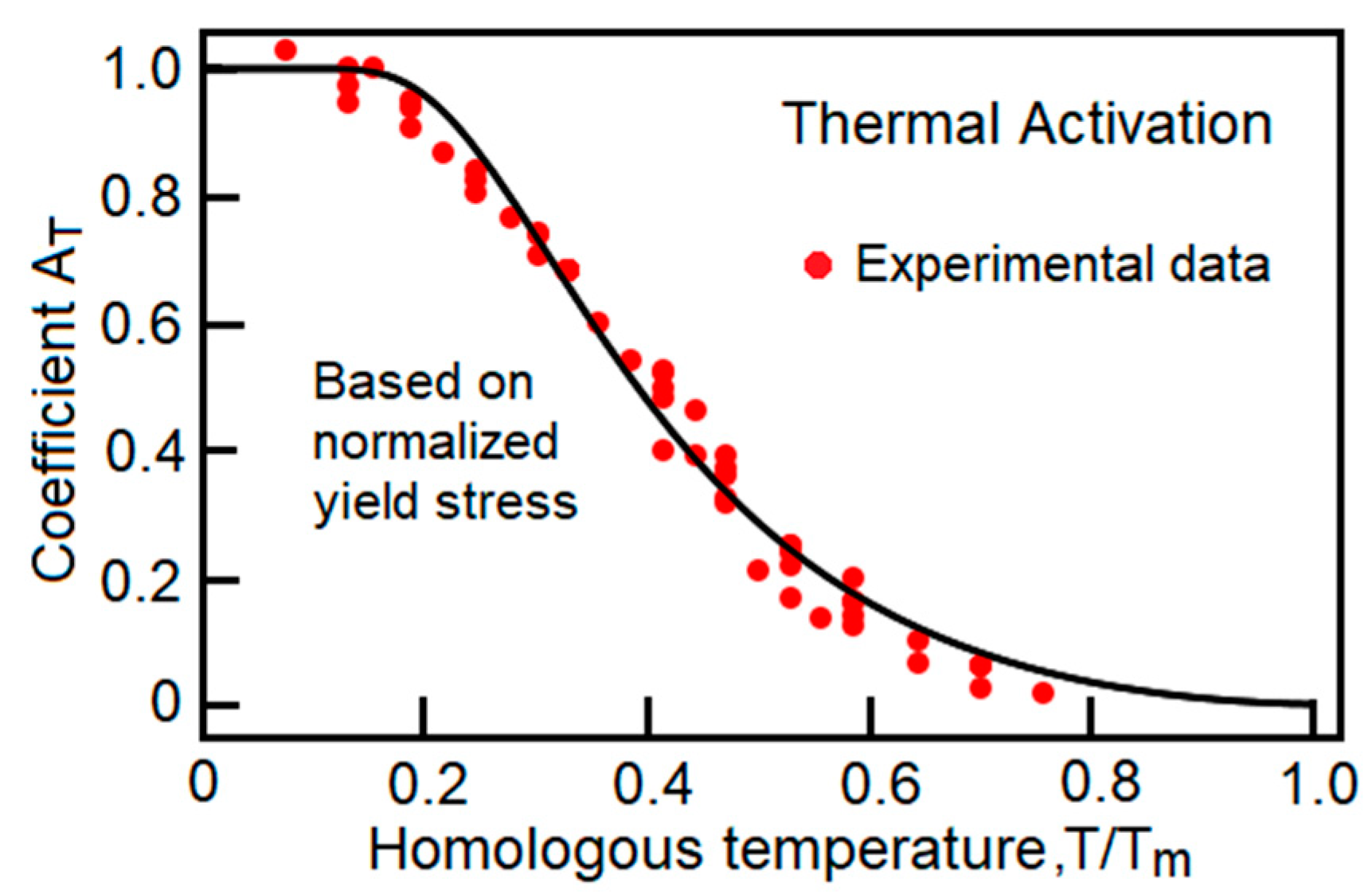
In previously tested metals, the non-dimensional parameter $g_a$ is found in the range of one, the transition temperature $T_c$ specifies the conversion of the power-law creep into the dislocation glide mechanism, and $T_m$ is the melting point. The exponent $k_a$ determines the rate of the thermally activated processes, and in face-centered cubic metals the exponent is much smaller than one. In bcc and hcp metals, the thermal activation is much stronger, and the exponent is somewhat greater than one. In Mg AZ31B alloy, the thermal activation coefficient is evaluated by plotting the yield stress as a function of temperature. In each set of data [7,14,15,16,17], the yield stress is normalized against the stress at room temperature. In the final step, the plot is rescaled such that $A_T\left(0\right)=1$ (Figure 1). The coefficient $A_T$ reaches a maximum value at very low temperatures and has an extended tail near the melting point. The constants used in the relation (2) are listed in

Table 1. Thermal activation.

Thermal Activation	${\mathit{g}}_{\mathit{a}}$	${\mathit{k}}_{\mathit{a}}$	${\mathit{T}}_{\mathit{m}}$	${\mathit{T}}_{\mathit{c}}$
$A_T$	$0.823$	$1.66$	$890 \mathrm{K}$	$0.588 T_m$

. The melting point is shown to be within the range of 878 K to 903 K. Here, we assume that $T_m=890 \mathrm{K}$.

4. Mechanism of Plastic Flow

We are ready to resume the TRM-based analysis, in which the Huber–von Mises flow tensor will be shown to have a clear geometric interpretation [12,18]. The mechanism is further generalized and adapted for Mg AZ31B. It is assumed that the eigentensors are expressed in terms of the stress deviator. We emphasize that the tensors satisfy the conditions: $tr{\mathit{N}}^1=tr{\mathit{N}}^2=tr{\mathit{N}}^3=1$, ${\mathit{N}}^1:{\mathit{N}}^2={\mathit{N}}^1:{\mathit{N}}^3={\mathit{N}}^2:{\mathit{N}}^3=0$, and ${\mathit{N}}^1+{\mathit{N}}^2+{\mathit{N}}^3=\mathbf{1}$. Thus, all the properties of the orthogonal triad are preserved. With that said, the flow tensor is presented in the following form:

$$\mathit{M}=\alpha \left[\left({\mathit{N}}^1-{\mathit{N}}^3\right)+{\mu }_{\phi }\left(\frac{1}{3}\mathbf{1}-{\mathit{N}}^2\right)\right].$$

(3)

The flow tensor was derived in [19]. In the expression, $\left({\mathit{N}}^1-{\mathit{N}}^3\right)$ captures the slip along the dominant shear plane, while ${\mu }_{\phi }\left(\frac{1}{3}\mathbf{1}-{\mathit{N}}^2\right)$ estimates the contribution of the non-planar slip. In Mg AZ31B, the non-planarity is a consequence of the slip-twinning interactions and the subsequent activation of screw dislocations [20,21]. The second term in (3) quantifies the atomistically resolved friction coefficient. The functions $\alpha$ and ${\mu }_{\phi }$ are derived by matching the flow tensor (3) with the mechanism $\mathit{M}=\mathit{S}/\sqrt{3J_2}$. In Equation (3), the condition $tr\mathit{M}=0$ is satisfied automatically, and the other two invariants are $tr{\mathit{M}}^2=6$ and $tr{\mathit{M}}^2=6 \sin \phi$. The functions are $\alpha =\sqrt{3}\cos \left(\phi /3\right)$ and ${\mu }_{\phi }=\sqrt{3}{\beta }_0\tan \left(\phi /3\right)$, where the angles $\phi ={\mathrm{s}\mathrm{i}\mathrm{n}}^{-1}\left(A_{\phi }\right)$ and $A_{\phi }=3\sqrt{3} J_3/\left(2 J_2^3\right)$ complete the relation. Again, the second and third invariants of the stress deviator are $J_2=tr{\mathit{S}}^2/2$ and $J_3=tr{\mathit{S}}^3/3$. The Huber–von Mises flow mechanism is recovered when the parameter ${\beta }_0$ is equal to one. The convexity of the stress envelope is preserved when the selected parameter is between $1$ and $1/2$. Here, ${\beta }_0=1$.

One may wonder, why complicate a seemingly simple problem? Would the expression $\mathit{M}=\mathit{S}/\sqrt{3J_2}$ be a simpler alternative? It turns out that the shape of the yield surfaces is sensitive to ${\beta }_0$. Thus, the yield criterion is generalized a great deal beyond the von Mises description. Additionally, the flow tensor (3) efficiently handles the directionality (anisotropy) of the plastic flow. Therefore, the expression (3) offers obvious advantages.

5. Plastic Anisotropy

Magnesium alloy AZ31B exhibits strong plastic anisotropy. A method developed in [18] is used here for the reconstruction of the directional flow. The concept can be explained as follows. Imagine that the material’s responses are monitored by two observers. One of them was immersed in the material prior to the rolling process and, therefore, the observer perceives the material to be elastically and plastically isotropic. Another observer is located outside the material. This second observer also monitors the deformation and realizes that the rolling process introduces texture which makes the plastic responses directional. The key idea here is to determine the transformation rules which correlate with the strains monitored by the two observers. In what follows, the rules are derived by projecting the texture-free basis onto the basis of the external observations. The externally detected strain ${\mathit{\epsilon }}^T$ is called the texture strain. It is the elastic strain ${\mathit{\epsilon }}^e$ projected onto the external reference system, hence:

$${\mathit{\epsilon }}^T={\epsilon }_{ij}^e\left[{\xi }_T^1\right(T_1^i{\mathit{e}}_i\otimes {\mathit{e}}_j{T}_1^j)+{\xi }_T^2\left(T_2^i{\mathit{e}}_i\otimes {\mathit{e}}_j{T}_2^j\right)+{\xi }_T^3\left(T_3^i{\mathit{e}}_i\otimes {\mathit{e}}_j{T}_3^j\right)]$$

(4)

where ${\mathit{e}}_i^T=T_i^j{\mathit{e}}_j$ and ${\mathit{e}}_i$ establish the orthogonal triad of the texture-free material. The dyads $T_1^i{T}_1^j$, $T_2^i{T}_2^j$, and $T_3^i{T}_3^j$ are symmetric and describe the transformation of the T-basis. It has been shown in [18] that the texture strain ${\mathit{\epsilon }}^T={\epsilon }_{ij}^e\left({\xi }_A^{ij} {\mathit{e}}_i\otimes {\mathit{e}}_j\right)$ carries complete information on the elastic and plastic directionalities, and that the information is stored in the coefficients ${\xi }_A^{ij}={\xi }_T^1 T_1^i{T}_1^j+{\xi }_T^2 T_2^i{T}_2^j+{\xi }_T^3 T_3^i{T}_3^j$. In the relations, the summation rule between ${\epsilon }_{ij}^e$ and ${\xi }_A^{ij}$ does not apply. Rolled sheets of AZ31B exhibit an in-plane directional property. Discounting elastic anisotropy, only three parameters characterize the plastic directionality. The in-plane parameters in the transverse, rolling, and shear directions ${\xi }_A^{11}$, ${\xi }_A^{22}$, and ${\xi }_A^{12}$ are calibrated, while the others must satisfy additional conditions, specifically ${\xi }_A^{11}+{\xi }_A^{22}+{\xi }_A^{33}=3$ and ${\xi }_A^{12}+{\xi }_A^{13}+{\xi }_A^{23}=3$. Thus, ${\xi }_A^{33}=3-{\xi }_A^{11}-{\xi }_A^{22}$ and ${\xi }_A^{13}={\xi }_A^{23}=\left(3-{\xi }_A^{12}\right)/2$.

In Equation (3), the flow tensor $\mathit{M}$ was expressed in terms of stress. In isotropic elastic material, the same result can be achieved by replacing stress with elastic strain ${\mathit{\epsilon }}^e$, that is, $\mathit{M}\left(\mathit{\sigma }\right)=\mathit{M}\left({\mathit{\epsilon }}^e\right)$. However, texture violates the co-directionality, which is $\mathit{M}\left({\mathit{\epsilon }}^T\right)\ne \mathit{M}\left(\mathit{\sigma }\right)$. The anisotropy is calibrated against the experimental data presented in [22]. Since the rate of plastic strain is ${\dot{\mathit{\epsilon }}}^p=\mathit{M}\left({\mathit{\epsilon }}^T\right){\dot{e}}^p/2$, where ${\dot{e}}^p$ is the rate magnitude, one can assess the flow directionality by writing $r_{\theta }=tr\left({\mathit{N}}_{\theta }·\mathit{M}\right)/tr\left({\mathit{N}}_w·\mathit{M}\right)$, where ${\mathit{N}}_{\theta }$ points in the $\theta$-direction between the rolling and transverse orientations. The tensor ${\mathit{N}}_w$ is constructed on a unit vector pointing in the direction perpendicular to the sheet’s surface. Note that $\left({\mathit{N}}_w+{\mathit{N}}_{\theta }+{\mathit{N}}_{\theta +\pi /2}\right):\mathit{M}=0$, and it is so because ${\mathit{N}}_w+{\mathit{N}}_{\theta }+{\mathit{N}}_{\theta +\pi /2}=1$. The three anisotropy coefficients are listed in

Table 2. Plastic anisotropy (parameters in rolling direction, transverse direction, and shear direction).

Plastic Anisotropy	${\mathit{\xi }}_{\mathit{A}}^{11}$	${\mathit{\xi }}_{\mathit{A}}^{22}$	${\mathit{\xi }}_{\mathit{A}}^{12}$
${\xi }_A^{ij}$	$1.820$	$0.965$	$1.584$

.

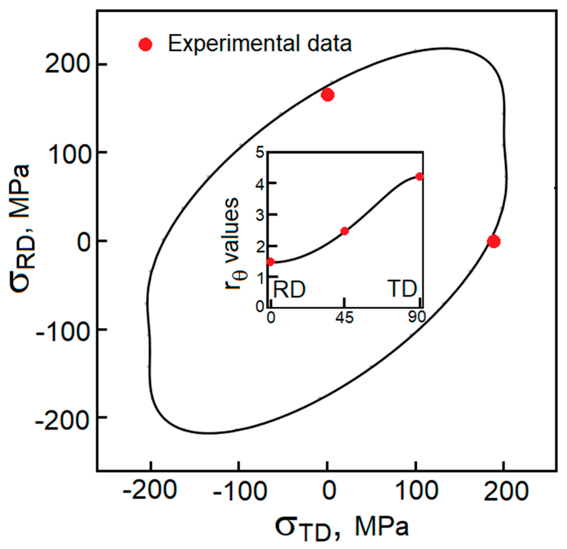
The stress envelope for Mg AZ31B is shown in Figure 2. The values of the tensile yield stresses in the TD and RD directions are obtained from [22]. The two points are placed on the stress envelope and are marked in red. Note that the shape of the surface is distorted. In addition, the instantaneous Lankford coefficient $r_{\theta }$ is plotted against three data points extracted from the same reference [22]. The instantaneous coefficients are taken at 2% of the plastic strain. The points are also marked in red. It is important to mention that the stress envelop can be evaluated in tension only. An in-plane compression activates the twinning mechanism, the crystallographic reorientations take over, and, as a result, the plastic flow is delayed.

6. Viscoplasticity

The plastic flow follows the direction established by the flow tensor $\mathit{M}\left({\mathit{\epsilon }}^T\right)$ and, as stated earlier, the flow magnitude is determined by the rate of plastic strain ${\dot{e}}^p$ such that ${\dot{\mathit{\epsilon }}}^p=\mathit{M} {\dot{e}}^p/2$. From the requirement of measure invariance (independence from the frame of description), we have ${\dot{W}}^p=\mathit{\sigma }:{\dot{\mathit{\epsilon }}}^p={\sigma }_{eq}{\dot{e}}^p$, and the equivalent stress becomes ${\sigma }_{eq}=\mathit{M}:\mathit{\sigma }/2$. The rate ${\dot{e}}^p$ is coupled with the equivalent stress through the power-law relation

$${\dot{e}}^p=m_S {\dot{\Lambda }}_p{\left(\frac{{\sigma }_{eq}-{\sigma }_r}{{\sigma }_p}\right)}^{n_p}.$$

(5)

The relation contains several variables. As always, the yield stress ${\sigma }_p$ is a temperature sensitive property, ${\sigma }_p={\sigma }_p^0 A_T,$ and the athermal strength ${\sigma }_p^0$ is evaluated at 0 K. The role of the residual stresses ${\sigma }_r$ is discussed first. The stress is a result of the interactions between the plastic slip and the twin boundaries. The stress sources can be located between grains, grain families, or twin–parent pairs [23]. Lastly, the stress can be affected by the penetration of dislocations into the extension twins [24]. The long-range back stress is responsible for the Bauschinger effect [25].The stress sources are integrated into the equation ${\sigma }_r={\alpha }_r\left(e_T^{max}/e_T^{lim}\right)A_T \mu ,$ where ${\alpha }_r$ is a constant, the ratio $e_T^{max}/e_T^{lim}$ quantifies the contribution of dislocation–twinning interactions, and $\mu$ is the shear modulus. The term $e_T^{max}/e_T^{lim}$ is further explained in the section on twinning. The magnitude of the residual stress is sensitive to temperature $A_T$.

The power-law relation controls the strain rate sensitivity through two exponents. Specifically, the stress exponent $n_p$ and the strain rate exponent ${\omega }_p$ in ${\dot{\Lambda }}_p={\dot{e}}_N^0{\left(\frac{{\dot{e}}_N^t+{\dot{e}}_{dif}}{{\dot{e}}_N^0}\right)}^{{\omega }_p}$, where ${\dot{e}}_N^t={\left({\dot{\mathit{\epsilon }}}^t:{\dot{\mathit{\epsilon }}}^t/2\right)}^{1/2}$. The characteristic strain rate ${\dot{e}}_{dif}$ projects the relation (5) into the regime of diffusional flow. At strain rates ${10}^{-4}/s$ and greater, the constant can be neglected. The strain rate exponent ${\omega }_p$ is equal to ${\omega }_p={A_T}^{0.05}$. Thus, the strain rate sensitivity varies with temperature. Note that the total, elastic, and plastic strains are ${\mathit{\epsilon }}^t$, ${\mathit{\epsilon }}^e$, and ${\mathit{\epsilon }}^p$, respectively.

The Schmid factor $m_S$ derived in [13,26] deserves an additional explanation. Let us assume that the angle $\theta =0$ is designated for the dominant slip plane. The spread of the angles is taken to be between $\pm \pi /4$, and the plane misorientations thus have clearly defined boundaries. The participation of misoriented planes in the plastic flow is evaluated according to the frequency of the slip occurrences $f_{\theta }\left(\theta \right)$. In hcp polycrystals, the broadening of the distribution results from the accommodation of the prismatic and pyramidal slip. The functional form $f_{\theta }\left(\theta \right)=\frac{2\Gamma \left(1+1/2r\right)}{\sqrt{\pi } \Gamma \left(1/2+1/2r\right)}{\cos }^{1/r}2\theta$ properly represents the problem, where ${\int }_{-\pi /4}^{\pi /4}{f}_{\theta }\left(\theta \right)d\theta =1$ and Γ is the gamma function. The exponent $r$ controls the shape of the distribution. The relationship between the slip-plane distribution and the Schmid factor was derived in [13] and is $m_S=m_g-m_r$, where $m_g\cong \frac{1+r}{1+\pi r/2}$ evaluates the arrangement of active slip systems, while $m_r=\frac{3 A_T\left(T\right)}{\pi \left(1+2 r\right)}$ quantifies the rate at which the reorganizations occur. The exponent $r$ reflects the advances of plastic strain and is assumed to be in a linear form, $r=r_0+e^p/e_r^p$.

Several points should be clarified. At low stresses, when ${\dot{\mathit{\epsilon }}}^e\cong {\dot{\mathit{\epsilon }}}^t$, the relation (5) can be simplified to ${\dot{e}}^p\propto {\left({\sigma }_{eq}^p/{\sigma }_0^p\right)}^{n_p}$. Under such conditions, the plastic flow becomes the diffusional flow. At the advanced stage of plastic deformation (stage III of plastic hardening), or during a constant-stress creep, when ${\dot{\mathit{\epsilon }}}^p\to {\dot{\mathit{\epsilon }}}^t$, the strain rate dependence is greatly reduced, ${\dot{e}}_{eq}\propto {\left({\sigma }_{eq}^p/{\sigma }_0^p\right)}^{n_p/\left(1-{\omega }_p\right)}$. For example, at a medium temperature range, the exponent is about ${\omega }_p=0.98$ and, therefore, the stress exponent is in the range of $n_p/\left(1-{\omega }_p\right)\approx 20$ and thus produces the familiar strain rate sensitivity. In this construction, the material experiences a smooth transition from diffusional flow ${\dot{e}}^p\propto {\left({\sigma }_{eq}^p/{\sigma }_0^p\right)}^{n_p}$ through power-law creep into dislocation glide ${\dot{e}}^p\propto {\left({\sigma }_{eq}^p/{\sigma }_0^p\right)}^{n_p/\left(1-{\omega }_p\right)}$. Note that at ${\omega }_p\to 1$, the material becomes rate insensitive (cryogenic temperatures). The constants for AZ31B are presented in

Table 3. Parameters used in the generalized viscoplasticity model.

Plastic Flow	${\mathit{\sigma }}_0^{\mathit{p}}$	${\mathit{n}}_{\mathit{p}}$	${\mathit{r}}_0$	${\mathit{e}}_{\mathit{r}}^{\mathit{p}}$	${\mathit{\alpha }}_{\mathit{r}}$	${\dot{\mathit{e}}}_{\mathit{d}\mathit{i}\mathit{f}}$
$A_T$	$288 \mathrm{MPa}$	$2.12$	$0.1$	$0.07$	$0.045$	$5\times {10}^{-5}/s$

. The back stress will be further evaluated in the section on twinning.

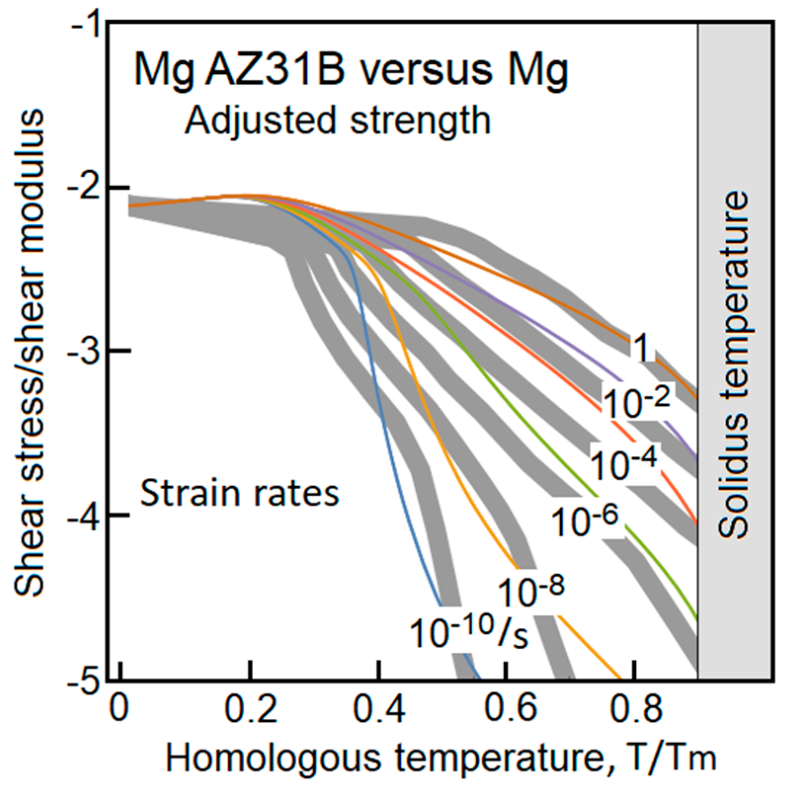
The viscoplastic relation (5) can describe metal responses within a broad range of conditions. For this reason, we were tempted to test the model against the Frost–Ashby deformation map for magnesium [27]. In the absence of a map for Mg AZ31B, the idea was to observe only the trends, where the yield stress for the alloy was scaled down. In Figure 3, the isolines of constant strain rate are marked by gray lines. Despite the obvious differences between the two materials, the two maps were found to be quite similar.

7. Crystallographic Reorientations

In rolled sheets of AZ31B alloy, the orientation of the c-axis is closely aligned with the sheet’s out-of-plane direction. Therefore, when such sheets are subjected to an in-plane compression, the loading produces tensile strain along the c-axis and, as a result, the elastic stretch activates crystallographic reorientations. Here, the c-axis direction is denoted by the unit vector ${\mathit{n}}^c$. The dyadic product ${\mathit{N}}^c={\mathit{n}}^c\otimes {\mathit{n}}^c$ establishes the first reference plane. When the extension twins are activated, there must be a lateral plane ${\mathit{N}}_T^3$, which jointly with ${\mathit{N}}^c$ defines the resolved shear plane $\left({\mathit{N}}^c-{\mathit{N}}_T^3\right)$. The two tensors, along with a third one, ${\mathit{N}}_T^2$, form an orthogonal triad, that is ${\mathit{N}}^c+{\mathit{N}}_T^2+{\mathit{N}}_T^3=\mathbf{1}$. This means that $tr\left({\mathit{N}}^c·{\mathit{N}}_T^3\right)=0$, $tr\left({\mathit{N}}^c·{\mathit{N}}_T^2\right)=0$, and $tr\left({\mathit{N}}_T^2·{\mathit{N}}_T^3\right)=0$. It should be emphasized that the orthogonality assumption does not apply for the contraction twins, where $tr\left({\mathit{N}}^c·{\mathit{N}}_{contraction}^3\right)\approx 0.75$. In our analysis, the contraction twins are blended into the residual twins, as is discussed later.

The orientation of the eigentensors ${\mathit{N}}_T^2$ and ${\mathit{N}}_T^3$ is controlled by the current elastic strain. The TRM enables the determination of the explicit relationship between ${\mathit{N}}_T^3$ and elastic strain ${\mathit{\epsilon }}^e$, such that ${\mathit{N}}_T^2={\mathit{N}}_T^2\left({\mathit{\epsilon }}^e\right)$, ${\mathit{N}}_T^3={\mathit{N}}_T^3\left({\mathit{\epsilon }}^e\right)$, and ${\mathit{N}}_T^2:{\mathit{\epsilon }}^e>{\mathit{N}}_T^3:{\mathit{\epsilon }}^e$. The following conditions must be satisfied:

$$\begin{array}{c}tr\left({\mathit{N}}^c·{\mathit{N}}_T^3\right)=0\\ {tr\mathit{N}}_T^3=1\\ tr{\left({\mathit{N}}_T^3\right)}^2=1\end{array}.$$

(6)

The eigentensor ${\mathit{N}}_T^2$ can be calculated from ${\mathit{N}}_T^2=\mathbf{1}-\left({\mathit{N}}^c+{\mathit{N}}_T^3\right)$. The mathematical expression for ${\mathit{N}}_T^3$ is presented in Appendix A.

The deformation caused by the extension twins follows the direction of maximum shear on the plane $\left({\mathit{N}}^c-{\mathit{N}}_T^3\right)$.Therefore, the rate of the instantaneously generated deformation is

$${\dot{\mathit{\epsilon }}}^{RT}=\left({\mathit{N}}^c-{\mathit{N}}_T^3\right) {\dot{e}}_T/2.$$

(7)

The strain rate ${\dot{e}}_T$ quantifies the rate at which the crystallographic reorientations occur. Locally, the process is rapid; the changes spread within grains but have a limited capacity for generating shear deformation. The resolved shear stress is calculated from the conjugate pair of stress and strain rate, $\mathit{\sigma }:{\dot{\mathit{\epsilon }}}^{RT}={\sigma }_T{\dot{e}}_T$ , and is ${\sigma }_T=\left({\mathit{N}}^c-{\mathit{N}}_T^3\right):\mathit{\sigma }/2$.

$${\sigma }_T=\left({\mathit{N}}^c-{\mathit{N}}_T^3\right):\mathit{\sigma }/2.$$

(8)

When the c-axis is in tension $\left({\epsilon }_c^e={\mathit{N}}^c:{\mathit{\epsilon }}^e>0\right)$, the resolved shear stress takes a positive value, ${\sigma }_T>0$. A negative sign indicates that the detwinning process might have begun. It is important to understand that the sign changes and that this feature makes the resolved shear stress different from the equivalent stress in plasticity. In addition, note that ${\mathit{N}}^c:\mathit{\sigma }$ and ${\mathit{N}}_T^3:\mathit{\sigma }$ are not principal stresses.

The rate of twinning is proportional to the resolved shear stress ${\sigma }_T$. The process can be activated when ${\epsilon }_c^e={\mathit{N}}^c:{\mathit{\epsilon }}^e>0$ and ${\sigma }_T>0$, granted that the resolved shear stress is in the range of ${\sigma }_T^0$. Moreover, the reorientations continue to occur until the deformation limit $e_T^{lim}$ is reached. Lastly, the twinning process can be activated when the crystal has the required capacity described here by the rate ${\dot{e}}_T^t=\sqrt{tr{\left({\dot{\mathit{\epsilon }}}^t-{\dot{\mathit{\epsilon }}}^p\right)}^2/2}$. Consequently, at the advanced stage of the plastic flow $\left({\dot{\mathit{\epsilon }}}^p\to {\dot{\mathit{\epsilon }}}^t\right)$, the twinning mechanism is shut down. All the requirements are integrated into the relation

$${\dot{e}}_T={\dot{e}}_T^t\frac{e_T^{lim}-e_R}{e_T^{lim}} {\xi }_T {\left({\sigma }_T/{\sigma }_T^0\right)}^{n_T}.$$

(9)

The twinning–detwinning condition is controlled by the parameter ${\xi }_T=(\left|{\epsilon }_c^e\right|+{\epsilon }_c^e)/(2\left|{\epsilon }_c^e\right|+{\delta }_{\epsilon })$, where ${\delta }_{\epsilon }$ is a small numerical number (in this study ${\delta }_{\epsilon }={10}^{-11}$). In short, the twins are generated when ${\xi }_T=1$, and the c-axis is in compression when ${\xi }_T=0$. The detwinning mechanism is defined by the sister relation

$${\dot{e}}_D={\dot{e}}_T^t\frac{e_T}{e_T^{lim}}{({\xi }_T-1){\left(\right|\sigma }_T\left|{/\sigma }_T^0\right)}^{n_T}.$$

(10)

The original (parent) crystallographic organization can be recovered, and this happens when the resolved shear stress takes a negative value $\left({\sigma }_T<0\right)$. The recovery process is limited by the availability of the shear strain $e_T$. In other words, only pre-existing twins can be erased, and when $e_T=0$, the process ends. Lastly, residual twins are produced at load reversals and during subsequent unloading [28]. Here, the mechanism is proposed in a simple linear form:

$${\dot{e}}_{TD}={\Lambda }_{TD}\frac{e_T^{max}}{e_T^{lim}}{\dot{\sigma }}_T/{\sigma }_T^0,$$

(11)

where $e_T^{max}=max\left\{e_T\right\}$ is the maximum magnitude of the twinning deformation generated during the entire loading process. In the relation, the production and/or annihilation of residual twins is solely dependent on the sign ${\dot{\sigma }}_T$. The load reversals create a condition for stretching the limit $e_T^{lim}$. In other words, the secondary twins enhance the material’s readiness for twinning. The effects are characterized by the maximum and minimum values of $e_{TD}$, i.e., $e_{TD}^{max}=max\left\{e_{TD}\right\}$ and $e_{TD}^{min}=min\left\{e_{TD}\right\}$, such that

$$e_T^{lim}=e_T^0+e_{TD}^{max}-e_{TD}^{min}.$$

(12)

The initial limit $e_T^0$ can be assessed under proportional loading and is in the range of 10% to 13%. The parameter ${\Lambda }_{TD}$ estimates the maximum strain generated by the residual twins. In summary, the current rate of twinning and detwinning includes three mechanisms, ${\dot{e}}_R={\dot{e}}_T+{\dot{e}}_D+{\dot{e}}_{TD}$, and the current state of the twinned polycrystal is defined as

$$e_R={\int }_0^t\left({\dot{e}}_D+{\dot{e}}_D+{\dot{e}}_{TD}\right)dt.$$

(13)

The mechanisms of twinning and detwinning are described in terms of four parameters. The parameters for AZ31B are listed in the

Table 4. List of parameters for the twinning/detwinning model. Parameters calibrated for Mg AZ31B alloy.

Twinning	${\mathit{\sigma }}_{\mathit{T}}^0$	${\mathit{n}}_{\mathit{T}}$	${\mathit{e}}_{\mathit{T}}^0$	${\mathbf{\Lambda }}_{\mathit{T}\mathit{D}}$
	$30 \mathrm{M}\mathrm{P}\mathrm{a}$	$3$	$0.108$	$0.0033$

.

As stated earlier (Equation (7)), the strain rate ${\dot{\mathit{\epsilon }}}^{RT}=\left({\mathit{N}}^c-{\mathit{N}}_T^3\right)\frac{{\dot{e}}_T}{2}$ reflects the active twinning mechanism. In a polycrystalline alloy, various reorientations, ${\mathit{N}}_T^3$, can be achieved, though the detwinning deformation must still follow the previously established trajectories. We realize that the deformation ${\mathit{\epsilon }}^{RT}$ represents the crystallographic state of the material. Additionally, the advances of ${\mathit{\epsilon }}^{RT}$ progressively settle the recovery pathways. For this reason, the instantaneously chosen planes $\left({\mathit{N}}^c-{\mathit{N}}_T^3\right)$ progressively mature the resolved shear plane $\left({\mathit{N}}_D^1-{\mathit{N}}_D^3\right)$, where ${\mathit{N}}_D^1={\mathit{N}}_D^1\left({\mathit{\epsilon }}^{RT}\right)$ and ${\mathit{N}}_D^2={\mathit{N}}_D^2\left({\mathit{\epsilon }}^{RT}\right)$ , while ${\mathit{N}}_D^1:{\mathit{\epsilon }}^{RT}>{\mathit{N}}_D^2:{\mathit{\epsilon }}^{RT}>{\mathit{N}}_D^3:{\mathit{\epsilon }}^{RT}$. As a result, we have 

$${\dot{\mathit{\epsilon }}}^r=\left({\mathit{N}}_D^1-{\mathit{N}}_D^3\right) {\dot{e}}_r/2.$$

(14)

This point is of paramount importance. The accumulated reorientations establish the path for a potential detwinning. Therefore, the strain ${\mathit{\epsilon }}^r$ determines the current twinning status in the material, while the strain ${\mathit{\epsilon }}^{RT}$ shows how the state was accomplished. Proportional loading makes the tensors $\left({\mathit{N}}^c-{\mathit{N}}_T^3\right)$ and $\left({\mathit{N}}_D^1-{\mathit{N}}_D^3\right)$ nearly identical. The differences become relevant in complex loading scenarios.

8. Discussion

The mechanisms of plastic flow and crystallographic reconfigurations are developed in the framework of the tensor representation method. It has been shown that plastic flow and deformation twinning are vastly different mechanisms. In dislocation plasticity, the active stimulus can be the current stress, the elastic strain, or the texture strain. Crystallographic reorientations are determined by the c-axis orientation and the elastic strain. The plasticity part of the model was used previously and was proven to capture the relevant behavior of AZ31B alloy. The twinning mechanism is a new addition.

In the literature, the viscoplastic self-consistent (VPSC) model is considered the most prominent simulation tool [29]. This tool has been proven to accurately predict the behavior of single crystals. Polycrystalline samples require additional fitting parameters, but the level of predictability is still undeniable. However, large-scale computational engineering must rely on numerically efficient constitutive models. Unfortunately, our phenomenological models for plasticity are ill-equipped to handle the complex behaviors of magnesium alloys. One reason is that plastic flow and deformation twinning are very different deformation mechanisms. Here, it has been shown that the TRM delivers the necessary tools for constructing these dissimilar deformation mechanisms. In the current study, the TRM connected the generic deformation mechanisms with the proper stimuli, captured relevant kinematical constraints, eliminated ad-hoc assumptions, and established well-defined rules for the tensorial structure of the model.

When studying the behaviors of magnesium alloys, we should be aware that the preprocessing treatment cannot be ignored. To avoid an unnecessary disparity in data, we made a conscious decision to rely on experimental data from a single source [22]. In the model, the isotropic elastic properties at room temperature are defined in terms of the shear modulus $\mu =\mathrm{17,000} \mathrm{M}\mathrm{P}\mathrm{a}$ and the bulk modulus $B=\mathrm{48,000} \mathrm{M}\mathrm{P}\mathrm{a}$. The elastic response $\dot{\mathit{\sigma }}=\mathit{C}·{\dot{\mathit{\epsilon }}}^e$ and the strain rate additivity ${\dot{\mathit{\epsilon }}}^t={\dot{\mathit{\epsilon }}}^e+{\dot{\mathit{\epsilon }}}^p+{\dot{\mathit{\epsilon }}}^r$ complete the constitutive description. The isotropic elastic tensor $\mathit{C}$ needs no further explanation.

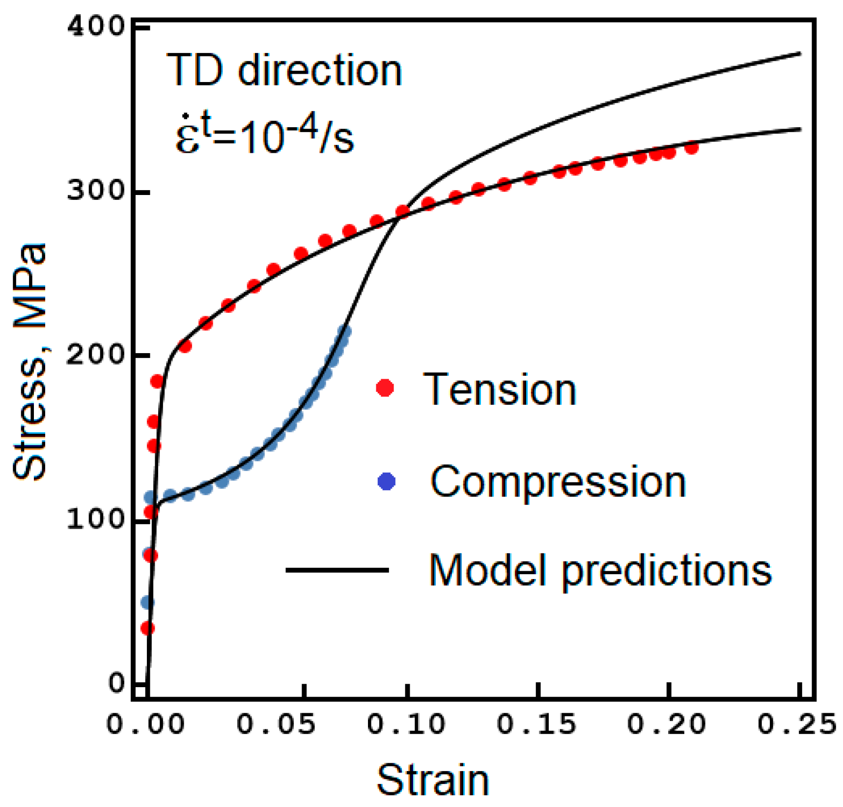
The plot in Figure 4 depicts uniaxial stress–strain responses in tension and compression. The experimental results [22] were obtained at the strain rate $~{10}^{-4}/\mathrm{s}$ and at room temperature. The sample was tested in the TD (transverse direction). In all cases, the sheets were 3.2 mm thick. The red dots denote the tension data and the blue dots represent the stress–strain response under compression. The solid lines designate the model predictions.

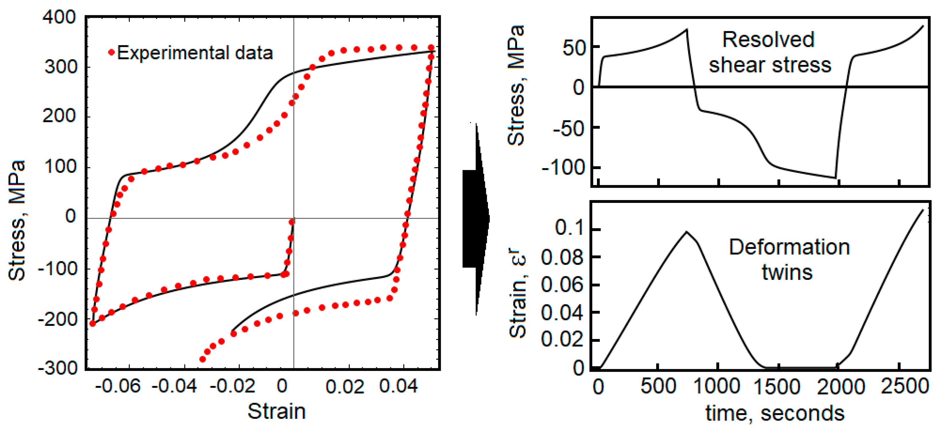
Next, the model is tested under cyclic conditions. In Figure 5, strain-controlled loading is applied under compression, and the load direction is then reversed twice. The twins initially accumulated under compression are fully recovered under tension. At the next reversal, the twinning process resumes. The red dots are the experimental data points collected from [22]. The right-hand side plots illustrate the twinning process. The twinning deformation is generated under compression, i.e., when the c-axis is in tension and ${\sigma }_T$ has a positive value. The resolved shear stress takes a negative value under tension. The plot displayed below shows the twinning and detwinning cycle presented as a function of time.

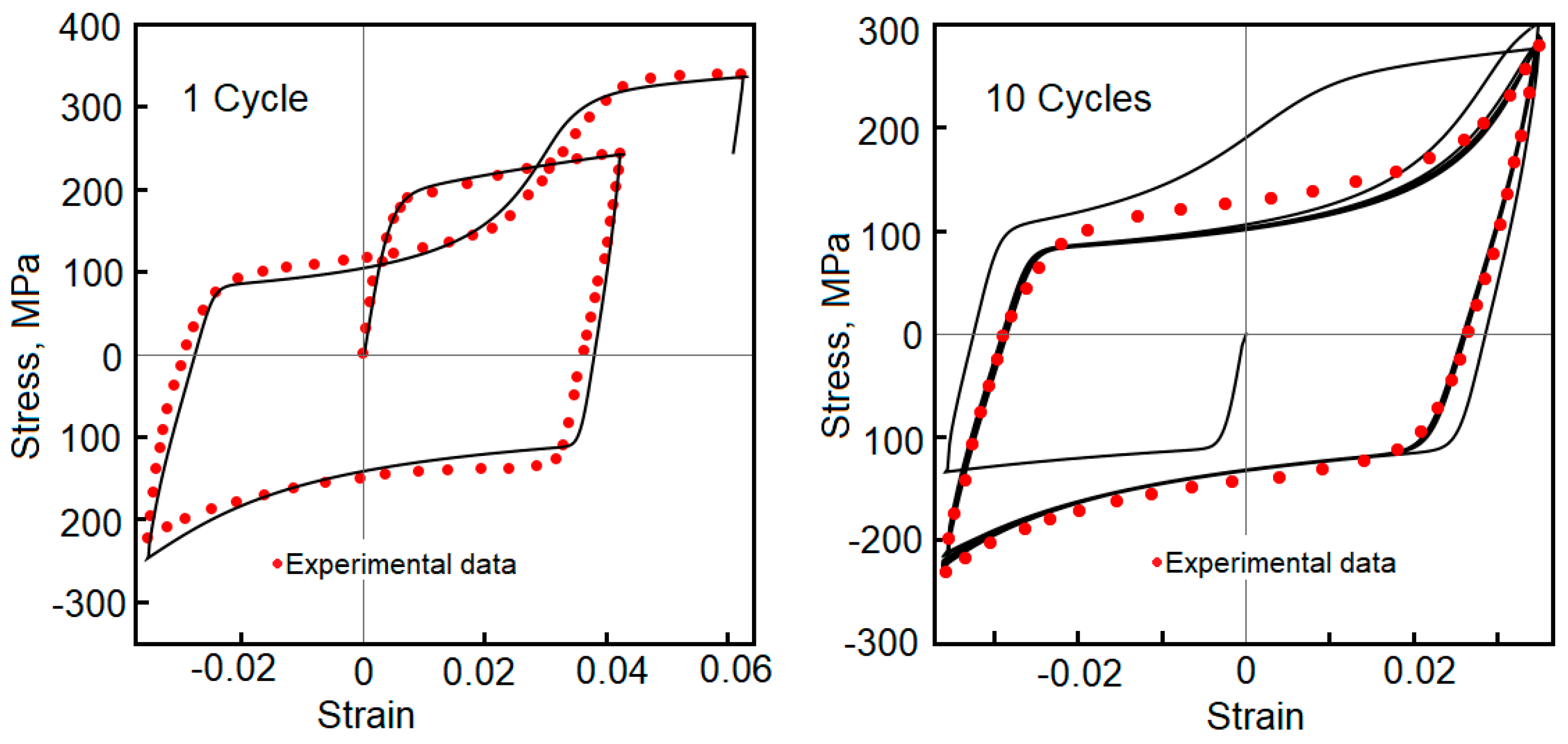
Lastly, two cases of strain-controlled cycles are calculated and compared with the experimental data [22]. On the left-hand side of Figure 6, the loading process begins under tension, and twins are thus not generated. After the load is reversed, the stress produces twins, which then are recovered under tension. In the second plot in Figure 6, a saturated cycle was obtained after the material was subjected to ten stress–strain reversals. As before, the red dots represent the experimental data from [22].

9. Conclusions

Two objectives inspired this study. On the one hand, the idea was to share the tensor representation method as applied to constitutive modeling. In the past, several models were developed, but the method itself was explained briefly, thus leaving some level of uncertainty for potential users. Here, several unpublished details have been included. The hope is that the TRM can become a useful tool that streamlines the development of constitutive models for a broad class of materials, such as polycrystalline metals, geomaterials, or polycrystalline polymers. It has been shown that twinning can be reproduced in a physics-based manner, and that its complexity can be reduced and its predictability enhanced. The second goal was to develop a simple and yet predictive constitutive model for Mg AZ31B alloy. The model was tuned for a textured alloy, where the hcp c-axes are oriented in one predominant direction. The plasticity part of the model included the viscoplastic flow rules and the highly directional flow mechanism. Additionally, the plasticity model captured the temperature sensitivity from the cryogenic environment up to the melting point, and the strain rates captured the diffusional flow up to the regime of mild dynamics. It is worth stating that a single equation for the viscoplastic flow can reproduce the entire Frost–Ashby deformation map [27]. It has also been shown that the twinning mechanism is described with the use of 4 parameters, and that each of them has a well-defined meaning. The temperature dependence of the twinning mechanism is yet to be established.

The constitutive description can be further enhanced to cover the regime of dynamic plasticity, as described in [30]. In addition, the TRM is very suitable for the development of fracture mechanisms under tension and compression, and this has been undertaken elsewhere [26].

References

- Zubelewicz, A. Micromechanical Study of Ductile Polycrystalline Materials. J. Mech. Phys. Solids 1993, 41, 1711–1722. [Google Scholar] [CrossRef]
- Zubelewicz, A.; Rougier, E.; Ostoja-Starzewski, M.; Knight, E.E.; Bradley, C.; Viswanathan, H.S. Dynamic behavior and fracture of materials. Int. J. Rock Mech. Min. Sci. 2014, 72, 277–282. [Google Scholar] [CrossRef]
- Zubelewicz, A.; Thompson, D.G.; Ostoja-Starzewski, M.; Ionita, A.; Shunk, D.; Lewis, M.W.; Lawson, J.C.; Kale, S.; Koric, S. Fracture model for cemented aggregates. AIP Adv. 2013, 3, 012119. [Google Scholar] [CrossRef]
- Zhang, X.; Li, B.; Wu, X.; Zhu, Y.; Ma, Q.; Liu, Q.; Wang, P.; Horstemeyer, M. Twin boundaries showing very large deviations from the twinning plane. Scr. Mater. 2012, 67, 862–865. [Google Scholar] [CrossRef]
- Zhang, D.; Jiang, L.; Zheng, B.; Schoenung, J.M.; Mahajan, S.; Lavernia, E.J.; Beyerlein, I.J.; Schoenung, J.M.; Lavernia, E.J. Chapter 02878 Deformation twinning (update). In Materials Science and Materials Engineering; Elsevier Inc.: Amsterdam, The Netherlands, 2016. [Google Scholar] [CrossRef]
- Lentz, M.; Risse, M.; Schaefer, N.; Reimers, W.; Beyerlein, I.J. Strength and ductility with — double twinning in a magnesium alloy. Nat. Commun. 2016, 7, 11068. [Google Scholar] [CrossRef] [PubMed]
- Agnew, S.R.; Duygulu, Ö. Plastic anisotropy and the role of non-basal slip in magnesium alloy AZ31B. Int. J. Plast. 2005, 21, 1161–1193. [Google Scholar] [CrossRef]
- Morrow, B.M.; McCabe, R.J.; Cerreta, E.K.; Tomé, C.N. In-Situ TEM Observation of twinning and detwinning during cyclic loading in Mg. Metall. Mater. Trans. A 2014, 45, 36–40. [Google Scholar] [CrossRef]
- Shi, D.; Zhang, J. Abnormal twinning behavior induced by local stress in magnesium. Materials 2022, 15, 5510. [Google Scholar] [CrossRef] [PubMed]
- Yoo, M.H. Slip, twinning, and fracture in hexagonal close packed metals. Metall. Trans. A 1981, 12, 409–418. [Google Scholar] [CrossRef]
- Morozumi, S.; Kikuchi, M.; Yoshinaga, H. Electron microscope observation in and around twins in magnesium. Trans. JIM 1976, 17, 158–164. [Google Scholar] [CrossRef]
- Zubelewicz, A.; Clayton, J.D. Yield surfaces and plastic potentials for metals, with analysis of plastic dilatation and strength asymmetry in BCC crystals. Metals 2023, 13, 523. [Google Scholar] [CrossRef]
- Zubelewicz, A.; Oliferuk, W. Mechanisms-based viscoplasticity: Theoretical approach and experimental validation for steel 304L. Sci. Rep. 2016, 6, 23681. [Google Scholar] [CrossRef]
- Koike, J.; Ohyama, R.; Kobayashi, T.; Suzuki, M.; Maruyama, K. Grain-boundary sliding in AZ31 magnesium alloys at room temperature to 523K. Mater. Trans. 2003, 44, 445–451. [Google Scholar] [CrossRef]
- Alexander, D.J. Materials for cold neutron sources: Cryogenic and irradiation effects. In Proceedings of the International WORKSHOP on Cold Neutron Sources, Los Alamos, NM, USA, 5–8 March 1990; Volume 23. RN:23079079. [Google Scholar]
- Nguyen, N.-T.; Seo, O.S.; Lee, C.A.; Lee, M.-G.; Kim, J.-H.; Kim, H.Y. Mechanical behavior of AZ31B Mg alloy sheets under monotonic and cyclic loadings at room and moderately elevated temperatures. Materials 2014, 7, 1271–1295. [Google Scholar] [CrossRef]
- Kim, J.H.; Kim, D.; Lee, Y.-S.; Lee, M.-G.; Chung, K.; Kim, H.-Y.; Wagoner, R.H. A temperature-dependent elasto-plastic constitutive model for magnesium alloy AZ31 sheets. Int. J. Plast. 2013, 50, 66–93. [Google Scholar] [CrossRef]
- Zubelewicz, A. Another perspective on elastic and plastic anisotropy of textured metals. Proc. R. Soc. A 2021, 477, 20210234. [Google Scholar] [CrossRef]
- Zubelewicz, A. Tensor representations in application to mechanisms-based constitutive modeling. In Report: ARA 2; Alek and Research Associates: Los Alamos, NM, USA, 2015. [Google Scholar] [CrossRef]
- Liu, Y.; Yan, J.; Xie, D.; Shen, Y.; Wang, J. Self-patterning screw <c> dislocations in pure Mg. Scr. Mater. 2021, 19, 86–89. [Google Scholar]
- Ahmad, R.; Wu, A.; Curtin, W.A. Analysis of double cross-slip of pyramidal I <c+a> screw dislocations in implications for ductility in Mg alloys. Acta Mater. 2020, 183, 228–241. [Google Scholar]
- Lou, X.Y.; Li, M.; Boger, R.K.; Agnew, S.R.; Wagoner, R.H. Hardening evolution of AZ31B Mg sheet. Int. J. Plast. 2007, 23, 44–86. [Google Scholar] [CrossRef]
- Louca, K.; Abdolvand, H.; Mareau, C.; Majkit, M.; Wright, J. Formation and annihilation of stressed deformation twins in magnesium. Commun. Mater. 2021, 2, 9. [Google Scholar] [CrossRef]
- Gong, W.; Zheng, R.; Harto, S.; Kawasaki, T.; Aizawa, K.; Aizawa, K. In-situ observation of twinning and detwinning in AZ31 alloy. J. Magnes. Alloy 2022, 10, 3418–3432. [Google Scholar] [CrossRef]
- Karaman, I.; Sehitoglu, H.; Chumlyakov, Y.I.; Maier, H.J.; Kireeva, I.V. The effect of twinning and slip on the Bauschinger effect of Hadfield steel single crystal. Metall. Mater. Trans. A 2001, 32, 695–706. [Google Scholar] [CrossRef]
- Zubelewicz, A. Mechanisms-based transitional viscoplasticity. Crystals 2020, 10, 212. [Google Scholar] [CrossRef]
- Frost, H.; Ashby, M.F. Deformation-Mechanism Maps: The Plasticity and Creep of Metals and Ceramics; Pergamon Press: Oxford, UK, 1982. [Google Scholar]
- Xie, Q.; Chen, Y.; Yang, P.; Zhao, Z.; Wang, Y.D.; An, K. In-situ neutron diffraction investigation on twinning/detwinning activities during tension-compression load reversal in a twinning induced plasticity steel. Scr. Mater. 2018, 150, 168–172. [Google Scholar] [CrossRef]
- Lebensohn, R.A.; Tomé, C.N. A self-consistent anisotropic approach. Acta Metall. Mater. 1993, 41, 2611–2624. [Google Scholar] [CrossRef]
- Zubelewicz, A. Thermodynamics description of dynamic plasticity in metals. Forces Mech. 2022, 9, 100121. [Google Scholar] [CrossRef]
Figure 1.
Thermal activation coefficient is plotted as a function of temperature from cryogenic temperature up to the melting point.
Figure 2.
A stress envelope is constructed for the plastically anisotropic sheet of Mg AZ31B alloy reported in [22]. The inner plot shows the Lankford coefficient plotted as a function of the angle between the rolling and transverse directions.
Figure 3.
Frost–Ashby deformation map for Mg AZ31B alloy compared with a reported map for pure magnesium [27].
Figure 4.
The stress–strain measurements are reproduced from [22]. The red dots represent the test results under tension and the blue dots refer to the test under compression. The tests were conducted in the TD at room temperature. The solid lines represent the model predictions.
Figure 5.
The stress–strain cycle reported in [22] is reproduced by the model. The red dots represent the test results. The test was conducted at room temperature and the strain-controlled loading was a slow process. The other two plots depict the resolved shear stress and the twinning deformation, both of which are constructed as a function of time.
Figure 6.
A single tension–compression cycle reported in [22] for Mg AZ31B alloy is reproduced (solid line). The red dots represent the test results. A cyclically saturated stress–strain response (10 cycles) for the same material is plotted on the right-hand side of the figure. All tests were conducted at room temperature.