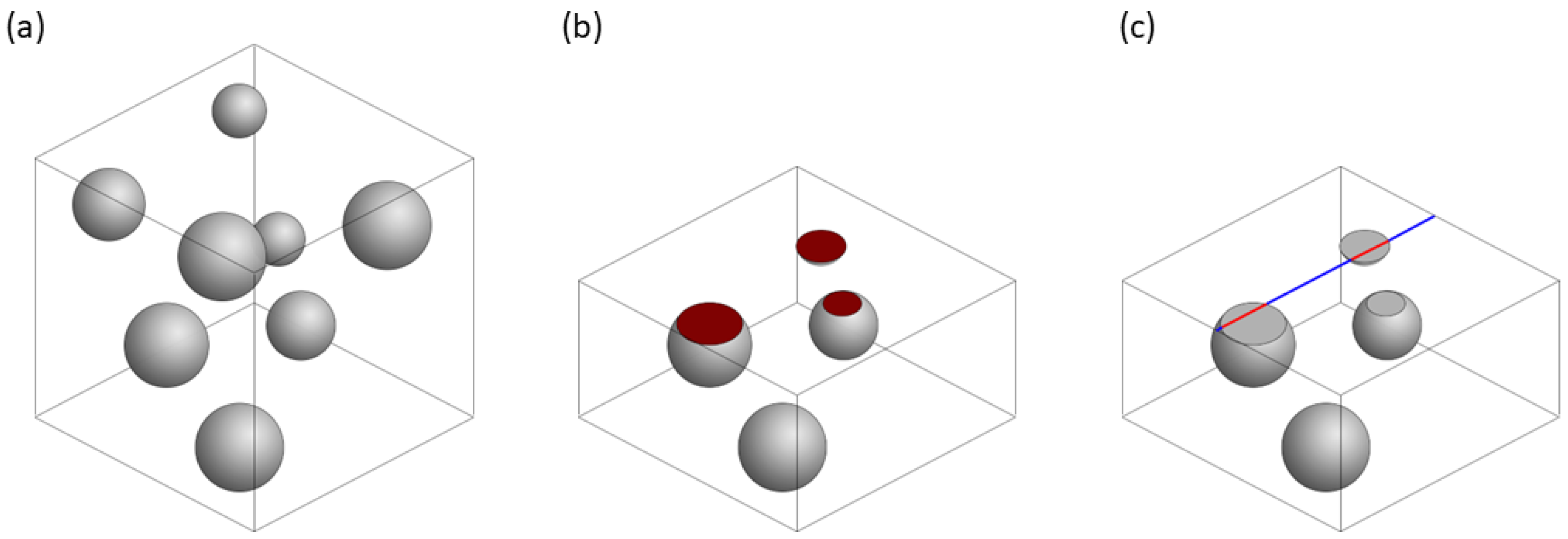
Article

Automated Stereology and Uncertainty Quantification Considering Spherical Non-Penetrating Dispersions

by
Magnus J. Anderson
* and
Hector C. Basoalto
Department of Materials Science & Engineering, The University of Sheffield, Mappin Street, Sheffield S1 3JD, UK
*
Author to whom correspondence should be addressed.
Crystals 2023, 13(3), 464; https://doi.org/10.3390/cryst13030464
Submission received: 6 February 2023 / Revised: 6 March 2023 / Accepted: 6 March 2023 / Published: 8 March 2023
(This article belongs to the Special Issue Mechanical and Microstructural Characterization of Superalloys)

Abstract

:
Automated stereological methods are presented for approximating the 3D size distribution of unimodal or bimodal precipitate dispersions considering 2D and 1D measurements taken from polydisperse spherical non-penetrating particle dispersions. A method to quantify the uncertainty of the approximation as a function of the number of sampled particles is presented and demonstrated to experimental data. The derivation and verification of the analytical stereological expressions used are included. Two procedures are presented for estimating the 3D size distribution of bimodal particle populations depending upon the relative size of the two particle populations. If the particles can be characterised using micrographs of the same magnification, it is possible to estimate the volume fraction of each particle population. For cases where micrographs have been taken at different magnification, an estimate of the area fractions of the particle populations is needed to combine the datasets and allow for the approximation of the 3D size distribution. These methods are useful for use in determining the initial particle size distribution for use in modelling and determining the appropriate number of micrographs and particles to measure when characterising a precipitate dispersion.

1. Introduction

Stereology describes the scientific approach to the approximation of the 3D size and morphology of objects utilising incomplete information. It is a fundamental aspect of microstructure characterisation and reconstruction [1]. Many microstructures are characterised through the quantitative image analysis of micrographs obtained from optical or scanning electron microscopy. These micrographs provide information descriptive of a 2D cross-section taken through the material. Serial sectioning is a powerful technique enabling the comprehensive characterisation of 3D microstructures exhibiting complex morphology, significant heterogeneity, and/or strong anisotropy [2]. For isotropic microstructures, information obtained from a single cross-section through the material is sufficient for a reasonable estimate of the morphology of the restructure. Microstructure reconstruction enables the quantitative analysis of the 3D size and morphology from such data [3].The approaches to microstructure reconstruction can be categorised as either optimisation-based approaches [4,5], texture synthesis [6,7], or machine-learning-based texture synthesis approaches [8,9]. Optimisation-based approaches apply inverse analysis to repetitively approximate the 3D microstructure, and then retrieve modelled data for a like-for-like comparison with the measured data to create the cost function. Texture synthesis approaches process the experimental data to reveal patterns and rules to use when reconstructing microstructure, reconstructing a new instance of the microstructure in one iteration. Bonstanabad et al. [8] replaced this with a neural network. This approach has significant computational savings once the network is adequately trained in comparison to optimisation-based approaches.
The focus of this work is the determination of the 3D size of non-penetrating polydisperse spherical particles using images descriptive of a cross-section through the dispersion. For this simple geometry an analytical solution [10,11] is available for the 3D → 2D conversion. This enables the use of optimisation-based approaches with small computational cost.
The shape descriptors used in this work include the equivalent radius of a circle with the same area as the identified object and the linear intercept. It is important to quantify the 3D size distribution of the precipitates when considering the kinetics of the evolution of the microstructural feature [12,13]. Gerlt et al. [14] have improved upon scaling factors used to approximate the mean 3D size and standard deviation from the mean 2D size and standard deviation obtained from a cross-section of the microstructure. They consider a unimodal dispersion where the shape of the particle size distribution is best captured by a log-normal distribution.
Precipitate dispersions that evolve following Ostwald ripening kinetics will reach a steady state where scaling laws can be applied to determine the continued evolution of the mean size of the precipitates [15,16]. Chen and Voorhees [17] studied the coarsening kinetics of precipitate dispersions and split behaviour into the transient and steady-state coarsening regimes. During the transient coarsening regime, the shape of the precipitate distribution may deviate from a log-normal type of distribution. Most precipitate strengthened alloys are heat treated to optimise the precipitate dispersion and often the dispersions needed for engineering applications are far from the steady-state regime. This work develops a method to consider any shape of the size distribution, in addition to multi-modal dispersions, applicable to both the transient and steady-state coarsening regimes.
Stereological functions for the 3D → 2D and 2D → 1D conversion of spherical precipitates are needed to understand and simulate the evolution of a precipitate dispersion [13,18,19]. For problems involving the coarsening or dissolution of an existing particle population, the ability to approximate the initial 3D size distribution is needed to simulate behaviour using mean-field models of kinetics. To compare predictions with experimental data taken from SEM or optical micrographs, either the predicted 3D particle size distributions need to be converted into 2D, or 3D size distributions of the experimental data need to be approximated for comparison with predictions.
Diogenes et al. [20] presented an optimisation-based procedure to approximate the 3D size of a non-penetrating dispersion of spheres from equivalent radii of circles obtained from a 2D intercept through the dispersion. They randomly cut discretely sampled particles from the approximated 3D distribution to build up a 2D distribution function to compare with the experimental data and explored different expressions to describe the 3D size distribution. They applied a simulated annealing algorithm to optimise the shape parameters to approximate the 3D size distribution.
This approach works well for unimodal distributions; however, multi-modal particle populations are encountered in many nickel-based superalloys. The aim of this work is to develop automated stereological methods to approximate the 3D size distribution of the bimodal particle populations observed in the turbine disc nickel superalloys RR1000 and IN738LC. The ability to approximate the initial particle size distribution is necessary for the application of mean-field modelling simulation tools such as TC-Prisma [21]. It is also useful in helping metallurgists determine the required number of micrographs to process and particles to measure to obtain sufficient confidence and understanding of the 3D size distribution of precipitates. Quantitative image analysis of micrographs to measure precipitate size and area fraction can be labour intensive and time consuming. Identifying the optimum number of micrographs to process and particles to measure can save time and improve the accuracy of measurements through knowledge of the error of the approximated 3D size distribution.
For completeness, the derivation of the analytical solution used to convert from 3D to 2D to 1D data is presented, arriving at the same result as Hilliard and Lawson [10] and Wicksell [11]. The derivation is verified against numerically generated results and then applied within an inverse calculation of the 3D size of unimodal and bimodal particle populations measured from scanning electron micrographs. A procedure to quantify the error associated with the 3D approximation is presented and then a discussion chapter notes other forms of error and uncertainty. The paper finishes with a conclusion, summarising the key findings.

2. Stereological Analytical Functions

2.1. Conceptual Framework

Let us consider a 3D volume containing polydisperse spherical precipitates. The number volume concentration of particles with radius varying between R and R + d R within a unit volume is given by the distribution function F 3 D ( R ) d R . Consider a cross-section taken through the particle dispersion. The number area concentration of cross-sections with a radius varying between r and r + d r is given by the distribution function F 2 D ( r ) d r . Let us then take a line through this plane. Let 2 l describe the linear intercept. The number line concentration of line intercepts with a length varying between l and l + d l is given by F 1 D ( l ) d l . This is illustrated in Figure 1.
The definitions used to define the geometry in 3D, 2D, and 1D are shown in Figure 2. The radius of the particle in 3D is given by R. The radius of a cross-section of a spherical particle is given by r, where a length of h has been removed, leaving a distance a between the cut surface and the particle centre. Figure 2c shows a line intercepting a particle with a length of 2 l is present within the particle cross-section.
The particle radius distribution function captures key statistics of the dispersion. The zeroth moment describes the number concentration within a volume, area, and line, considering the 3D, 2D, and 1D distribution functions, respectively. Let φ 3 D , φ 2 D , and φ 1 D refer to the volume fraction, area fraction, and line fraction of particles, respectively. For non-penetrating spherical particle ensembles, it is true that φ 3 D φ 2 D φ 1 D . Let R , r , and l describe the mean sizes encountered in the 3D, 2D, and 1D domains. This statistical information is obtained from the following moments of the size distribution functions
R = 0 R F 3 D d R 0 F 3 D d R φ 3 D = 4 π 3 0 R 3 F 3 D d R N v , 3 D = 0 F 3 D d R
r = 0 r F 2 D d r 0 F 2 D d r φ 2 D = π 0 r 2 F 2 D d r N a , 2 D = 0 F 2 D d r
l = 2 0 l F 1 D d l 0 F 1 D d l φ 1 D = 2 0 l F 1 D d l N l , 1 D = 0 F 1 D d l
Normalised probability distribution functions are obtained by normalising the F 3 D , F 2 D , and F 1 D by their zeroth moment
f 3 D = F 3 D 0 F 3 D d R f 2 D = F 2 D 0 F 2 D d r f 1 D = F 1 D 0 F 1 D d l
If the volume fraction, area fraction, or line fraction of particles is known, it is simple to calculate the F 3 D , F 2 D , and F 1 D functions from knowledge of the f 3 D , f 2 D , and f 1 D functions. For example, the 3D particle radius distribution can be obtained from the normalised probability distribution function as follows;
F 3 D = φ 3 D A f 3 D A = 4 π 3 0 R 3 f 3 D d R
and for the 2D particle radius distribution function;
F 2 D = φ 2 D A f 2 D A = π 0 r 2 f 2 D d r
and for the 1D particle intercept distribution function;
F 1 D = φ 1 D A f 1 D A = 2 0 l f 1 D d l
The particle number concentration can also be used in a similar manner to determine the size distribution functions from size probability density functions.
The functions that convert the 3D → 2D and 2D → 1D distribution functions are derived by calculating the mean particle radius of the cross-sections and line intercepts. The conversion functions are revealed by using the property that the mean value of a probability density is given by its first moment. The functions are determined for a monodisperse particle system and then extended to the polydisperse case.

2.2. 3D→2D Conversion

Hilliard and Lawson [10] show how to derive analytical expressions to convert a 3D particle size distribution to 2D area intercepts and 1D line intercepts. This work presents a different derivation that reaches the same result.
First, let us consider a 3D mono-disperse particle system containing particles of radius R. A plane cutting through the dispersion will result in a distribution of cross-sections of cut particles. Figure 2b illustrates the cut particle of radius R. The particle is cut by a distance of h resulting in a cross-section of radius r. Let the distribution of radii of cross-sections created by the plane be defined by the vector r k , with the corresponding vector n k describing the number of particles falling within each size interval. If there are m many size classes, the largest particle class in the distribution is given by r m = R . The mean particle radius for the monodisperse scenario is then defined by
r m = r 1 n 1 + r 2 n 2 + r 3 n 3 + . . . + r m n m n 1 + n 2 + n 3 + . . . + n k = k = 1 m r k n k η
where η = k = 1 m n k and is the total number of particle cross-sections found on the plane. The term n k / η is the probability that the plane intercepts a particle at the location within the distance between h and h + d h . Thus, the probability is given by n k / η = d h / R , and d h is a small increment of h described in Figure 2b. This allows Equation (8) to be expressed as
r m = k = 1 m r k d h R
Using these definitions for the geometry, the following is true
R 2 = R h k 2 + r k 2 a k 2 + r k 2
where h k and a k refer to the distances h and a defined in Figure 2b for the kth particle intercepted by the plane. Equation (10) may be arranged for a and differentiated with respect r to obtain,
d a d r k = r k R 2 r k 2
As d h = d a , we can express Equation (11) in terms of d h
d h = r k R 2 r k 2 d r k
Equation (12) is then substituted into Equation (9)
r m = k = 1 m r k r k R R 2 r k 2 d r k
We can convert Equation (13) into an integral under the limit d r k 0
r m = lim d r k 0 k = 1 m r k r k R R 2 r k 2 d r k = 0 R r r R R 2 r 2 d r
Revealing the 3D→ 2D conversion function
ξ ( R , r ) = r R R 2 r 2
The mean radius of cross-sections for the monodisperse system is given by
r m = 0 R r ξ ( R , r ) d r
We now extend the approach to a consider a polydisperse particle population. The mean radius of particle intersections can be determined by the summation of the particle size classes that cover the size range of particles present within the system. Let the vector R j define the mean radius of the size classes, and N j describe the number of particles within each size range, with a total of n particle size classes. The mean radius of the cross-sections obtained from the cut through the microstructure is given by
r p = N 1 r ( R 1 ) m + N 2 r ( R 2 ) m + N 3 r ( R 3 ) m + . . . + N l r ( R n ) m N 1 + N 2 + N 3 + . . . + N n
where r m and r p refer to the mean particle radius of cross-sections from a monomodal and a polydisperse ensemble, respectively. We can use the normalised probability density describing the particle radius distribution of 3D particles to determine N k
N k i = 1 n N i = f 3 D ( R k ) d R k
where d R k is the range of the size class of particles N k . Equation (17) may now be expressed as
r p = k = 1 n f 3 D ( R k ) r ( R k ) m d R k
Substitute Equation (16) into Equation (19)
r p = k = 1 n f 3 D ( R k ) 0 R k r ξ ( R k , r ) d r d R k
The summation can be converted into an integral as d R k 0
r p = 0 f 3 D ( R ) 0 R r ξ ( R , r ) d r d R
The order in which the integral is performed may be switched, and the integral manipulated, to arrive at
r p = 0 r r f 3 D ( R ) ξ ( R , r ) d R d r
Revealing the following 3D→2D conversion function for a polydisperse ensemble
f 2 D ( r ) = r f 3 D ( R ) r R R 2 r 2 d R
This is the same result as Hilliard and Lawson [10] and Wicksell [11].

2.3. 2D→1D Conversion

The same process can be followed to determine the conversion to 1D data from 2D data. Let us now consider the distribution of line intercepts present in a 2D system of monodisperse circles. The geometry of the line intercept is given in Figure 2c), where the line intercept present in the particle phase is given by 2 l . Following the same procedure, the following 1D distribution function is obtained
f 1 D ( l ) = r f 2 D ( r ) l r r 2 l 2 d r

3. Model Verification

The functions shown in Equation (15) consider the cross-sections of a single size of particle. Figure 3 compares the analytical ξ ( R , r ) function to numerically generated data considering a particle with a radius of 1m. The numerical solution is obtained by using a pseudo-random number generator to take cross-sections or intersections through the particle, binning the radius of the cut into a histogram, and then converting the histogram into a probability density.
The polydisperse analytical 3D → 2D and 2D → 1D functions are applicable to any f 3 D distribution function. They have been tested against numerically generated distributions of equivalent radii and linear intercepts using a pseudo-random number generator to sample the distribution and create the distribution of cross-sections and linear intercepts. Table 1 lists the expressions used to create particle dispersions to verify the conversion. The parameter σ is the standard deviation and μ is the mean of the normal and log-normal distributions. The term ζ is the fraction weighting applied to the distributions in the bimodal case. The parameters used in the Weibull waveform include γ , which is an offset of the distribution, α , which impacts the distribution shape, and β , which determines the mean of the distribution.
Figure 4 compares the numerically calculated 2D and 1D distribution functions descriptive of the equivalent radius and linear intercept for the four distribution functions described in Table 1. The parameters used to define the 3D distribution functions are outlined in Table 2. It can be seen that the analytical solution agrees with numerically generated data for a variety of distribution shapes and unimodal and bimodal distributions. Equation (23) has been applied to the f 3 D ( R ) distribution function to obtain an approximation of f 2 D ( r ) . Equation (24) is then applied to the predicted f 2 D distribution function to determine the f 1 D ( l ) distribution function.

4. Automated 3D Approximations of Spherical Particle Dispersions

4.1. Inverse Analysis

This section presents the algorithms for the objective functions used in the inverse analysis of the size distribution of both unimodal and bimodal dispersions. These are implemented using the optimisation algorithms provided in MATLAB [22,23] and Python [24]. The default optimisation routines are used, which are the simplex method and the Broyden–Fletcher–Goldfarb–Shanno (BFSG) algorithm, respectively. Exploration of different optimisation routines is beyond the scope of this work; however, there are differences in the converged solutions comparing the two techniques. First, the processing of the raw data is described to determine suitable approximations for the initial guess. Next, the objective functions for the inverse analysis are described. Examples are presented for approximating the 3D particle size distribution from scanning electron micrographs taken from precipitate dispersions in nickel superalloys. The last section presents a method for quantifying the error and uncertainty as a function of the sample size of precipitate measurements.

4.2. Unimodal Dispersions

The inverse calculation involves the calibration of the unknown parameters α , β , and γ for the Weilbull waveform shown in Equation (28). The measured 2D data can be used to approximate the initial guess of the parameters. The mean 3D particle radius of the Weibull equation presented in Table 1 is given by
R 3 D = 0 f 3 D R d R = γ + β Γ 1 + 1 α
where Γ is the gamma function.
Let us introduce the parameter K to relate the mean 2D intercept radius with the mean 3D radius of the spheres, so that R 3 D = K R 2 D . Let R 2 D * describe the mean radius of cross-sections measured from the experimental data. For the initial guess, we can approximate K = 4 / π . The γ parameter in the Weibull Equation describes an offset applied to the distribution. We can express the offset by the term ψ , which is normalised by the measured R 2 D * . The initial guess for γ can be expressed as a function of the parameter ψ and the measured mean 2D particle radius, so that
γ 4 π ψ R 2 D *
where 0 < ψ < 1 . The initial guess for β can now be obtained by rearranging Equation (29) for β and substituting Equation (31). The resulting equation may be rearranged to arrive at
β 4 R 2 D * 1 ψ π Γ 1 + 1 α
This reduces the number of variables for the initial guess from three parameters to two; α and ψ . An initial guess of 2.5 has been used for α , and 0.5 for ψ .
Upper and lower limits are needed for the optimisation of the unknown parameters α , β , and γ . Two times the maximum measured 2D particle size can be used to define the upper bounds for β and γ . The α parameter has been constrained between the interval of 1.5 and 10.
Inverse analysis requires an objective function which returns an absolute scalar value descriptive of the error. The error may be calculated from the integral of the absolute error between the measured and predicted 2D distributions. This can be achieved by comparing the measured and modelled particle radius distribution functions or the associated cumulative distribution function, p 2 D , as shown below:
error = r m i n r m a x | f 2 D data ( r ) f 2 D model ( r ) | d R error = r m i n r m a x | p 2 D data ( r ) p 2 D model ( r ) | d R
where r m i n and r m a x are the minimum and maximum radii of the measured 2D data of particle cross-sections. f 2 D data ( r ) and f 2 D model ( r ) are the 2D particle radius probability distribution functions obtained from the experimental data and model, respectively. p 2 D data ( r ) and p 2 D model ( r ) are the cumulative frequency densities associated with the f 2 D data ( r ) and f 2 D model ( r ) probability distribution functions. To enable the comparison of the data and model, the modelled 2D particle size distribution function f 2 D model ( r ) is linearly interpolated onto the same discretisation used to define the data, or vice versa, when the cumulative frequency density functions are used to quantify the error.
One problem encountered when comparing predicted f 2 D model ( r ) and measured f 2 D data ( r ) distribution functions is that the measured data is limited by the minimum particle that can be detected. There are numerous causes for this limitation, such as those arising from the microscopy technique, to the resolution of precipitations within the micrograph. As a result, there is always error comparing the left-hand tail of the f 2 D model ( r ) distribution with the f 2 D data ( r ) distribution where no data exists. In this work, we avoid this issue by only comparing data between the limits of r m i n and r m a x and scaling the predicted distribution so that, within these size intervals, the zeroth moment of the distribution moment is unity.
An example application of applying the automated stereological method is shown in Figure 5, where (a) and (b) show the identified particles from scanning electron micrographs taken from commercially cast IN738LC aged at 900 C for 10,000 h [13], and the primary particle population in air-quenched fine grain RR1000 [18]. The microstructures of interest contain a γ phase and globular γ precipitates. Figure 5c,d show the measured 2D particle size distributions for IN738LC and RR1000 and compared with the calibrated 2D and 3D distributions obtained from the inverse analysis. The figures compare model predictions from using the simplex method and BFSG algorithm. In both examples, the results from the simplex method predict a larger 3D size distribution, with a smoother left-hand tail. In both cases, the simplex method converged to a solution with lower error compared to the BFSG algorithm. The steps taken to create the objective function considering a unimodal dispersion using the accumulative probability density are described in Algorithm 1.
Algorithm 1 Unimodal 3D→2D approximation
  • Create f 3 D model for the latest approximation of α , β and γ .
  • Convert f 3 D model to f 2 D model .
  • Interpolate f 2 D model onto the same grid spacing as the experimental data.
  • Calculate the accumulative frequency density p 2 D model .
  • Calculate the relative absolute error comparing p 2 D model and p 2 D data .
  • Return the integral of the relative absolute error.

4.3. Bimodal Dispersions

The method has been extended to consider bimodal distributions. Although the previous unimodal approach could be applied for each individual particle population, this would not account for overlap of the larger 2D particle size distribution with the smaller particle size distribution. It would not account for the fact that a small cross-section on the 2D plane could come from either particle population in the bimodal distribution. Two scenarios have been considered depending upon the relative difference in size between the particle populations:
  • The bimodal particle populations have comparable size and both precipitate populations can be resolved on the same micrographs. A vector of measured particle radii is obtained describing both particle populations and a clear cut-off in size is identified splitting the two populations.
  • The particle populations vary in size by an order of magnitude and both particle populations cannot be effectively characterised at the same magnification. Two vectors of particle radii have been measured for each dispersion and the area fraction of the particle populations has been approximated.
The characterisation of the evolution of the bimodal gamma prime population in IN738LC [13] to a unimodal dispersion is used for an example of particles characterised using the first method. The gamma prime dispersion in as-heat-treated coarse grain RR1000 [18] is used as an example for the latter.
First, let us consider approximating the 3D size from data from each particle population that can be simply combined. In this case, two Weibull distributions are used with a fraction ζ i used to determine the weighting from each particle population. This is shown in Equation (33).
f 3 D ( R ) = i = 1 2 ζ i α i β i R γ i β i α i 1 e x p R γ i β i α i
There are seven unknown parameters that are calculated: the α i , β i and γ i shape parameters of the ith particle population and either ζ 1 or ζ 2 , as ζ 1 + ζ 2 = 1 . A cut-off that separates the two particle populations in the experimental data is useful in providing reasonable estimates for the initial guesses for these parameters.
One way to approach this problem would be to calculate both Weibull curve parameters at the same time, with seven unknown parameters using the cumulative probability density to determine the error in the objective function. The results are shown in Figure 6, which presents the calibrated probability density functions and cumulative distribution functions, respectively. Algorithm 2 presents the steps taken within the objective function.
Algorithm 2 Simultaneous bimodal 3 D 2 D approximation
  • Create two f 3 D model distributions for the latest approximation of α 1 , α 2 , β 1 , β 2 , γ 1 , γ 2 , and ζ 1 .
  • Convert both f 3 D model distributions to f 2 D model
  • Combine both f 2 D model dispersions using ζ 1 and ζ 2 to weight the populations.
  • Interpolate the combined f 2 D model onto the same grid spacing as experimental data
  • Calculate p 2 D model considering particles greater than the smallest available from the experimental data.
  • Calculate the relative absolute error comparing p 2 D model and p 2 D data .
  • Return the integral of the relative absolute error.
Another approach is to examine each population sequentially, starting with the largest population and then proceeding through the populations in descending order of size. This allows for 2D particle cross-sections that arise from the larger population of particles to be accounted for when examining the smaller particle populations. It is slightly faster than the previous method, needing to calibrate three parameters for the larger particle population ( α 1 , β 1 and g a m m a 1 ), and then four parameters ( α 2 , β 2 , g a m m a 2 , and ζ 2 ) for the secondary population. The probability density function has been used to determine to determine the error that defines the objective function. The results are shown in Figure 7. In this approach, Algorithm 1 is first applied to the largest population of particles to approximate their size distribution. Algorithm 3 is then used to approximate the smaller particle population.
Algorithm 3 Sequential bimodal 3D→2D approximation
  • Input the known f 2 D model particle size distribution for the primary particles obtained from applying Algorithm 1 to the primary dispersion in addition to f 2 D data describing both populations.
  • Create the f 3 D model distribution for the latest approximation of α , β , and γ for the secondary particles.
  • Convert the f 3 D model for the secondary particle distribution into f 2 D model .
  • Use the estimated ζ 1 term to combine both f 2 D model dispersions.
  • Interpolate the combined f 2 D model onto the same grid spacing as experimental data
  • Calculate the relative absolute error comparing f 2 D model and f 2 D data .
  • Return the integral of the relative absolute error.
The second case considered is when the two particle populations vary significantly in size. A high magnification micrograph is needed to measure the smaller particles accurately, but, if the same magnification was used to assess the larger particles, the sample size would be too small. Micrographs can be taken at different magnifications to characterise each population separately. Knowledge of the area fraction or number concentration of each type of particles allows for the datasets to be combined. In this case the area fraction of each population was approximated.
The example used is the as-heat-treated coarse grain RR1000 presented by Anderson et al. [18]. A vector of particle sizes and the approximated area fraction of each population was determined. The vectors of particle sizes have been transformed into histograms and then probability densities. Knowledge of their area fraction allows the determination of the distribution functions using Equation (6). The same histogram bin sizes are used to assess both populations so that the resultant distribution functions can be combined.
When the mean size between particle populations varies significantly, the magnitude of the particle radius distribution function can vary significantly for each population, incurring loss of significance issues. This can be addressed by viewing the particle distribution function in G ( R ) or g ( r ) space, were the particle radius number density concentration is weighted by the volume or area of the particle, as described in the following equations
G 2 D ( r ) = π F 2 D ( r ) r 2 g 2 D ( r ) = A 1 f 2 D ( r ) r 2 G 3 D ( R ) = 4 π 3 F 3 D ( R ) R 3 g 3 D ( R ) = A 1 f 3 D ( R ) R 3
where g 2 D ( r ) and g 3 D ( R ) are probability density functions. The term A is an integration constant that ensures that the zeroth moment of g 2 D ( r ) and g 3 D ( R ) is unity. The error used to define the objective function is performed in g 2 D ( r ) space
e r r o r = r m i n r m a x | g 2 D data g 2 D model | d r
Figure 8 shows an example application of this approach, approximating the 3D size distributions for the secondary and tertiary particles in fine grain RR1000 comparing results obtained from the simplex and BFSG methods. The figure presents the size distributions using the area fraction and volume fraction weighted space, as shown in Equation set (34). Figure 8a compares the measured 2D distribution of particle cross-sections extracted from the micrographs with the inverse analysis of the 3D distribution obtained from using the BFSG algorithm and Simplex method. Figure 8b shows the associated 3D distributions. There is a significant difference in the width of the distributions, with the Simplex method capturing the right-hand tail of the data more closely than the BFSG algorithm, with reduced error. The algorithm is described below, and applies Algorithm 1 to approximate the particle size distribution of the largest particle population first; however, it converts the f 2 D distribution into F 2 D with knowledge of the area fraction of the larger particles. This is then converted into G 2 D . Algorithm 4 is used to approximate the smaller particle population.
Algorithm 4 Simultaneous bimodal 3D→2D approximation using g space
  • Input the known G 2 D model particle size distribution for the primary particles obtained from applying Algorithm 1 in addition to g 2 D data describing both populations. Note that the G 2 D model distribution function captures the area fraction of primary particles.
  • Create the f 3 D model distribution for the latest approximation of α , β , and γ .
  • Convert the f 3 D model for the secondary particle distribution into f 2 D model .
  • Use the approximation of the area fraction of secondary particles to convert f 2 D model to F 2 D model .
  • Reformulate F 2 D model for the secondary particles into G 2 D model .
  • Combine the G 2 D model functions for the primary and secondary particles.
  • Normalise the combined G 2 D model function to a g 2 D model function.
  • Interpolate the combined g 2 D function onto the same grid spacing as experimental data
  • Calculate the relative absolute error comparing g 2 D model and g 2 D data .
  • Return the integral of the relative absolute error.

4.4. Error Quantification

A method was developed to assess the error as a function of the sample size. The method involves first approximating the 3D size distribution and using this approximation to re-sample the 2D distribution function numerically, and then re-calculating the 3D dispersion from the newly sampled 2D data. This is repeated, sampling the new 2D particles from the initial 3D approximation until sufficient data has been generated to assess the scatter and variation in the predicted 3D dispersion.
The algorithm is presented in Figure 9. The input data are the measurements of the radii of particles observed from cross-sections through the dispersion of interest. An initial inverse calculation is performed to approximate the 3D size, f 3 D . Particles are then repeatedly sampled from f 3 D using the same number of sampled particles as the measured data. Each time, the sampled particles are then cut to create a vector of cross-sectional radii. This is then used as the input for the inverse calculation of the 3D particle size distribution f 3 D * . The output is the calibrated parameters for the Gaussian waveform used to define f 3 D * . This process is repeated until sufficient statistics are obtained to capture the variation and uncertainty in the approximation of the 3D size distribution.
The method is demonstrated using the example considering the bimodal γ distribution in as-heat-treated IN738 shown in Figure 6, which was obtained with a total of 2748 particle measurements. Figure 10 shows the error associated with the predicted volume fraction of primary and secondary particles. This error is of a similar magnitude to the error encountered when quantifying microstructural features obtained from image-processing of micrographs. For example, the variation in area fraction comparing quantified micrographs taken in IN738LC is 5%, which is comparable to the extremes of ±2.5% observed in the secondary particles in Figure 10b. It would have a significant impact upon any calculation of mechanical properties that utilise the data.
The impact of the sample size upon error and uncertainty was assessed, varying the sample size from 300 to 30,000. For each sample size considered, the inverse calculation was repeated 15,000 times to generate the scatter and variation presented in Figure 11. This figure shows a continuous field of percentiles descriptive of the variation in the predicted G 3 D ( R ) distribution functions, where symmetry is applied around the 50th percentile, so that the same colour represents the 2nd and 7th percentiles.
Extreme error and uncertainty is shown for a sample size of 300, which is sometimes used to quantify unimodal distributions. This has a significant impact upon the estimated 3D number concentration, mean size, and volume fraction of the different populations, as shown in Figure 12. Figure 12a,b presents the scatter in predicted 3D mean particle radius and 3D number concentration considering the total distribution. Figure 12c,d present the variation in mean size and volume fraction of the primary particles, and Figure 12e,f show the scatter in mean size and volume fraction for the secondary particles. A sample size of less than 1000 results in unacceptable error in all the statistics examined. A sample size of 3000 particles is a reasonable number of particles; however, it still results in considerable uncertainty in particle volume fraction in the bimodal distribution, as shown in Figure 10, with 5% variation considering the 5th and 95th percentiles.
The method has been applied to quantify the error and uncertainty arising from sample sizes for the measurements taken to quantify the coarsening kinetics of γ in the nickel superalloy IN738LC [13]. The results are shown in Figure 13, using the same sample size as obtained from the quantitative image processing of the micrographs taken from the aged specimen.

5. Discussion

For unimodal precipitate dispersions, where the size distribution can be approximated as log-normal, the mean 3D size and standard deviation can be accurately estimated using the approach of Gerlt et al. [14]. If the distribution deviates from log-normal, the approach of Diogenes et al. [20] has the advantage that they can be easily modified to use different expressions to approximate the 3D size distribution. This work shows how such an approach can capture bi-modal dispersions. Improved computation time and accuracy can be achieved by using the analytical solutions to the 3 D 2 D conversion opposed to numerically sampling and cutting precipitates. This approach can be extended to capture more particle populations by following the same procedure, starting with the largest particle population and then performing inverse analysis on each population sequentially in order of descending particle size. The algorithms presented focus on using 2D information; however, it is trivial to perform the 2 D 1 D conversion and perform the analysis using 1D linear intercept measurements instead of 2D equivalent circular radii.
Although the error arising from the sample size has been investigated, there are many other sources of error and uncertainty when considering the approximation of the 3D size distribution of γ precipitates utilising SEM backscatter micrographs. The electrons that produce the image penetrate the sample, so that the image is not a true cross-section of the sample [25]. The voltage used to scan the image determines the depth of the electron penetration. Subsurface precipitates can be identified by their gradual transition into the matrix, compared with sharp interfaces for particles closer to the surface [26]. The etching of the matrix to reveal the precipitate phase also contributes to error when approximating the SEM backscatter image as a clean cross-section through the matrix [27]. The etching process can remove small particles and further reveal larger particles, impacting the observed 2D distribution [18]. Error may also arise from several issues associated with taking the image, ranging from poor focusing of the microscope impacting image quality to defects present from sample preparation.
The method discussed in this paper focuses on spherical precipitates, whilst the γ dispersions used as an example can vary considerably in morphology [28].
The geometry of some of the primary γ precipitates shown in Figure 5b deviate from spheres. Kruk et al. [2] and Pinz et al. [3] demonstrate the need to perform advanced characterisation and full-field microstructure reconstruction to fully understand the morphology and size of γ precipitate dispersions when it is no longer reasonable to estimate their geometry as spherical.

6. Conclusions

The analytical expressions for the 3D → 2D particle size distribution conversion and 2D → 1D particle size distribution conversion are presented for use in reconstructing spherical non-penetrating particle systems. The descriptions and implementations have been verified using a range of shapes for the particle size distribution, including normal, bimodal, log normal, and Weibull Gaussian functions. The 3D, 2D, and 1D size distribution function shapes show significant differences in shape, demonstrating the importance of correct stereological treatment when analysing measured size distributions from experimental data. Algorithms for the approximation of the 3D size distribution of bimodal particle size distributions have been developed and applied to the measurements of RR1000 and IN738LC. Multi-modal precipitate dispersions are commonly encountered in nickel-based superalloys used in turbine disc applications. They are critical components within a turbine engine, and the microstructure and properties must be fully understood.
A method for quantifying uncertainty in the approximated 3D size distribution is presented as a function of the sample size of measured particles. The approximated 3D particle size distribution is repetitively randomly sampled for particles using the same sample size as the characterisation, determining the error in mean size, standard deviation, and volume fraction of each particle population.
The method has been applied to the characterised dispersions in IN738LC [13], revealing an error as high as ±2.5% for the volume fraction of secondary particles. This is significant and impacts the accuracy of calculations of precipitate strengthening [29].
The approach approximates the geometry of the precipitates as spherical, which may not be accurate for the conditions and alloy of interest.

Author Contributions

Conceptualization, H.C.B.; methodology, M.J.A. and H.C.B.; software, M.J.A. and H.C.B.; validation, M.J.A. and H.C.B.; writing—original draft preparation, M.J.A. and H.C.B.; writing—review and editing, M.J.A. and H.C.B.; visualization, M.J.A. All authors have read and agreed to the published version of the manuscript.

Funding

This research received no external funding.

Data Availability Statement

The data that has been generated in this study are available on reasonable request from the corresponding author.

Conflicts of Interest

The authors declare no conflict of interest.

Nomenclature

The following nomenclature is used in this manuscript:
g 3 D ( R ) The probability density form of the G 3 D ( R ) function. It describes the probability density that a volume containing a particle has a radius varying within the range of R and R + d R ( 1 / m )
G 3 D ( R ) The probability density that a volume contains a particle with a radius varying between R and R + d R . ( 1 / m )
g 2 D ( r ) The probability density form of the G 2 D ( r ) function. It describes the probability density that an area containing a particle has a radius varying within the range of r and r + d r ( 1 / m ). ( 1 / m )
G 2 D ( r ) The probability density that an area contains a particle with a radius varying between r and r + d r . ( 1 / m )
p 2 D ( r ) The accumulative frequency density associated with the f 2 d ( r ) distribution function.
ψ The γ parameter normalised by the mean measured particle radius used to determine the initial approximation of Weibull parameters.
Γ The gamma function.
β A scale parameter that adjusts the size in the Weibull distribution function. (m)
γ A shift parameter that offsets the distribution in the Weibull distribution function. (m)
α A shape parameter used in the Weibull distribution function.
ζ i A weighting applied to individual distributions in multi-modal distribution functions, where the sum of ζ is unity and 0 < ζ i < 1 .
μ The expectation value of the distribution function. (m)
σ The standard deviation of the normal and log-normal distribution function. (m)
ξ The 3D→2D conversion function. ( 1 / m )
gThe distance between the particle surface and a line intersecting the particle, considering a line coincident with the particle centre as illustrated in Figure 2. (m)
hThe distance between the particle surface and the cutting plane intersecting the particle, considering a line coincident with the particle centre as illustrated in Figure 2. (m)
bThe distance between the particle centre and a line intersecting the particle as illustrated in Figure 2. (m)
aThe distance between the particle centre and a cutting plane intersecting the particle as illustrated in Figure 2. (m)
η The total number of cross-sections created by a plane intersected a system of spherical particles.
n i ( r i ) The number of particle cross-sections created by a plane intersected a system of spheres that have a radius of r i .
AAn integration constant.
N v , 1 D The line concentration of particle segments created by a line cutting through a 3D dispersion of particles. ( 1 / m )
N v , 2 D The area concentration of particle intersections created by a plane cutting through a 3D dispersion of particles. ( 1 / m 2 )
N v , 3 D The volume concentration of particles. ( 1 / m 3 )
l A half of the mean size of line segments created by the intersection of a line through a dispersion of spheres within a 3D volume. (m)
r The mean size of circles created by the intersection of a plane through a dispersion of spheres within a 3D volume. (m)
R The mean size of spheres present within a 3D volume. (m)
f 1 D ( l ) The probability density that a line intersecting a particle has a length varying between the closed interval of 2 l and 2 l + 2 d l that. ( 1 / m )
f 2 D ( r ) The probability density that the radius of a particle cross-section created by the intersection of a plane through a 3D ensemble of spherical particles has a radius varying between r and r + d r . ( 1 / m )
f 3 D ( R ) The probability density that a given particle has a radius varying between R and R + d R . ( 1 / m )
lHalf the length of a line intersecting a particle. (m)
rThe radius of an intersection created by cutting a sphere by a plane. (m)
RThe 3D radius of spheres present in the volume. (m)
ϕ 1 D The line fraction of particles.
ϕ 2 D The area fraction of particles.
ϕ 3 D The volume fraction of particles.
F 1 D ( l ) The concentration density of line segments of length 2l found when a line intersects through a dispersion of spheres. ( 1 / m 2 )
F 2 D ( r ) The radius distribution function describing the size density of circles of radius r created by the intersection of a plane through a system of spheres considering a unit area. ( 1 / m 3 )
F 3 D ( R ) The number concentration density of particles that have a radius varying between R and R + d R . ( 1 / m 4 )

References

  1. Bostanabad, R.; Zhang, Y.; Li, X.; Kearney, T.; Brinson, L.C.; Apley, D.W.; Liu, W.K.; Chen, W. Computational microstructure characterization and reconstruction: Review of the state-of-the-art techniques. Prog. Mater. Sci. 2018, 95, 1–41. [Google Scholar] [CrossRef]
  2. Kruk, A.; Dubiel, B.; Czyrska-Filemonowicz, A. The 3D imaging and metrology of CMSX-4 superalloy microstructure using FIB-SEM tomography method. In Solid State Phenomena; Trans Tech Publications Ltd.: Bäch, Switzerland, 2013; Volume 197, pp. 89–94. [Google Scholar]
  3. Pinz, M.; Weber, G.; Lenthe, W.; Uchic, M.; Pollock, T.; Ghosh, S. Microstructure and property based statistically equivalent RVEs for intragranular γ-γ’ microstructures of Ni-based superalloys. Acta Mater. 2018, 157, 245–258. [Google Scholar] [CrossRef]
  4. Yeong, C.; Torquato, S. Reconstructing random media. Phys. Rev. E 1998, 57, 495–506. [Google Scholar] [CrossRef] [Green Version]
  5. Seibert, P.; Raßloff, A.; Ambati, M.; Kästner, M. Descriptor-based reconstruction of three-dimensional microstructures through gradient-based optimization. Acta Mater. 2022, 227, 117667. [Google Scholar] [CrossRef]
  6. Wei, L.Y.; Levoy, M. Fast texture synthesis using tree-structured vector quantization. In Proceedings of the 27th Annual Conference on Computer Graphics and Interactive Techniques, New Orleans, LA, USA, 23–28 July 2000; pp. 479–488. [Google Scholar]
  7. Chen, Y.; Lin, L.; Sun, L.; Xie, X.; Ma, Z. 2-D microstructure characterization and reconstruction of heterogeneous materials based on combination of physical descriptor and texture synthesis. Mater. Charact. 2023, 196, 112585. [Google Scholar] [CrossRef]
  8. Bostanabad, R.; Chen, W.; Apley, D. Characterization and reconstruction of 3D stochastic microstructures via supervised learning. J. Microsc. 2016, 264, 282–297. [Google Scholar] [CrossRef]
  9. Jung, J.H.; Lee, S.J.; Kim, H.S. Estimation of Average Grain Size from Microstructure Image Using a Convolutional Neural Network. Materials 2022, 15, 6954. [Google Scholar] [CrossRef]
  10. Hilliard, J.E.; Lawson, L. Stereology and Stochastic Geometry; Springer Science & Business Media: Berlin/Heidelberg, Germany, 2003; Volume 28. [Google Scholar]
  11. Wicksell, S.D. The corpuscle problem: A mathematical study of a biometric problem. Biometrika 1925, 17, 84–99. [Google Scholar]
  12. Coakley, J.; Basoalto, H.; Dye, D. Coarsening of a multimodal nickel-base superalloy. Acta Mater. 2010, 58, 4019–4028. [Google Scholar] [CrossRef]
  13. Anderson, M.; Rowe, A.; Wells, J.; Basoalto, H. Application of a multi-component mean field model to the coarsening behaviour of a nickel-based superalloy. Acta Mater. 2016, 114, 80–96. [Google Scholar] [CrossRef] [Green Version]
  14. Gerlt, A.; Criner, A.; Semiatin, S.; Wertz, K.; Payton, E. Non-linear Transfer Functions for Accurately Estimating 3D Particle Size, Distribution, and Expected Error from 2D cross-sections of a Lognormal Distribution of Spherical Particles. Metall. Mater. Trans. A 2020, 52, 1–14. [Google Scholar] [CrossRef]
  15. Lifshitz, I.M.; Slyozov, V.V. The kinetics of precipitation from supersaturated solid solutions. J. Phys. Chem. Solids 1961, 19, 35–50. [Google Scholar] [CrossRef]
  16. Wagner, C.Z. Theorie der alterung von niederschlagen durch umlonsen (Ostwald-reifung). Z. Elektrochem. 1961, 65, 581–591. [Google Scholar]
  17. Chen, M.K.; Voorhees, P.W. The dynamics of transient Ostwald Ripening. Modell. Simul. Mater. Sci. Eng. 1993, 1, 591–612. [Google Scholar] [CrossRef]
  18. Anderson, M.; Schulz, F.; Lu, Y.; Kitaguchi, H.; Bowen, P.; Argyrakis, C.; Basoalto, H. On the modelling of precipitation kinetics in a turbine disc nickel based superalloy. Acta Mater. 2020, 191, 81–100. [Google Scholar] [CrossRef]
  19. Fahrmann, M.; Metzler, D. Simulation of γ’ precipitation kinetics in a commercial Ni-base superalloy. JOM 2016, 68, 2786–2792. [Google Scholar] [CrossRef]
  20. Diogenes, A.N.; dos Santos, L.O.E.; Fernandes, C.P. Particle size distribution correction method using a simulated annealing technique. Rev. Eng. Térmica 2011, 10, 38–43. [Google Scholar] [CrossRef]
  21. Andersson, J.O.; Helander, T.; Höglund, L.; Shi, P.; Sundman, B. Thermo-Calc & DICTRA, computational tools for materials science. Calphad 2002, 26, 273–312. [Google Scholar]
  22. MATLAB, Version R2022a; The MathWorks Inc.: Natick, MA, USA, 2022.
  23. D’Errico, J. Fminsearchbnd. 2022. Available online: https://www.mathworks.com/matlabcentral/fileexchange/8277-fminsearchbnd-fminsearchcon (accessed on 7 April 2020).
  24. Jones, E.; Oliphant, T.; Peterson, P. SciPy: Open Source Scientific Tools for Python. 2001. Available online: https://www.bibsonomy.org/bibtex/24b71448b262807648d60582c036b8e02/neurokernel (accessed on 6 September 2021).
  25. Payton, E.J.; Mills, M.J. Stereology of backscatter electron images of etched surfaces for characterization of particle size distributions and volume fractions: Estimation of imaging bias via Monte Carlo simulations. Mater. Charact. 2011, 62, 563–574. [Google Scholar] [CrossRef]
  26. Österreicher, J.A.; Grabner, F.; Schiffl, A.; Schwarz, S.; Bourret, G.R. Information depth in backscattered electron microscopy of nanoparticles within a solid matrix. Mater. Charact. 2018, 138, 145–153. [Google Scholar] [CrossRef]
  27. Smith, T.M.; Bonacuse, P.; Sosa, J.; Kulis, M.; Evans, L. A quantifiable and automated volume fraction characterization technique for secondary and tertiary γ’ precipitates in Ni-based superalloys. Mater. Charact. 2018, 140, 86–94. [Google Scholar] [CrossRef]
  28. Mitchell, R.; Hardy, M.; Preuss, M.; Tin, S. Development of γ’ Morphology in P/M Rotor Disc Alloys During Heat Treatment. Superalloys 2004, 361–370. [Google Scholar]
  29. Galindo-Nava, E.; Connor, L.; Rae, C. On the prediction of the yield stress of unimodal and multimodal γ’ Nickel-base superalloys. Acta Mater. 2015, 98, 377–390. [Google Scholar] [CrossRef] [Green Version]
Figure 1. (a) A 3D particle dispersion. (b) A cross-section through the dispersion, cutting through particles. (c) A line intercept passing through particles.
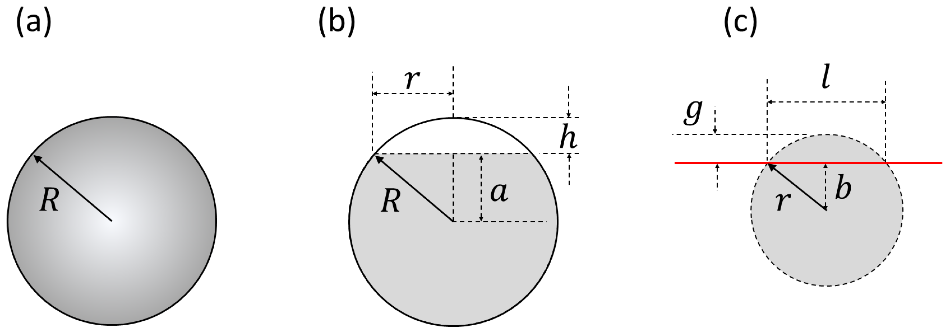
Crystals 13 00464 g001
Figure 2. The key geometry defining (a) the sphere, (b) the cross-section of a spherical particle, (c) the line intercept taken through a circle cross-section of a particle.
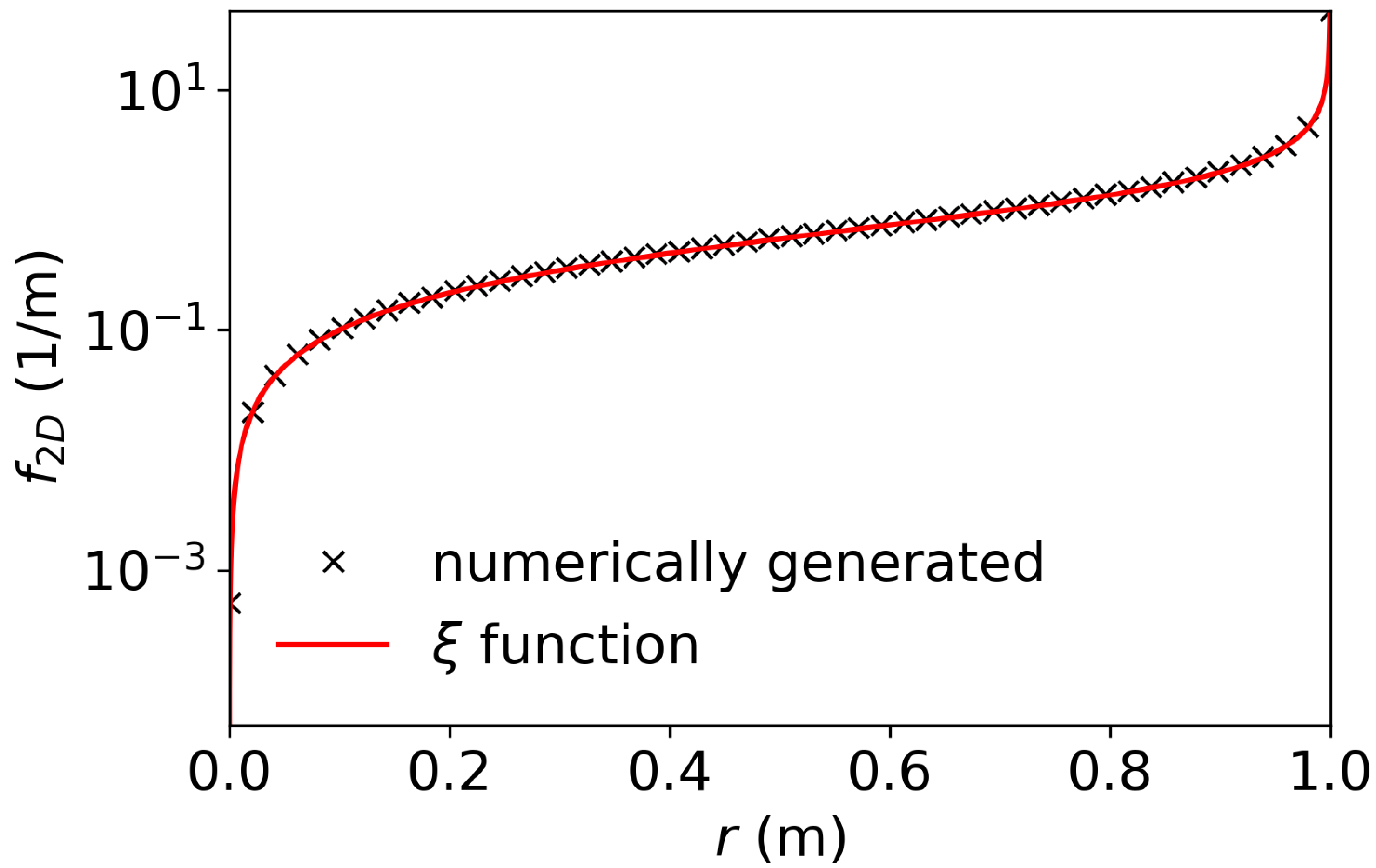
Crystals 13 00464 g002
Figure 3. Comparison of the numerically and analytically generated f 2 D distribution functions Equation (15) for a monodisperse particle ensemble.
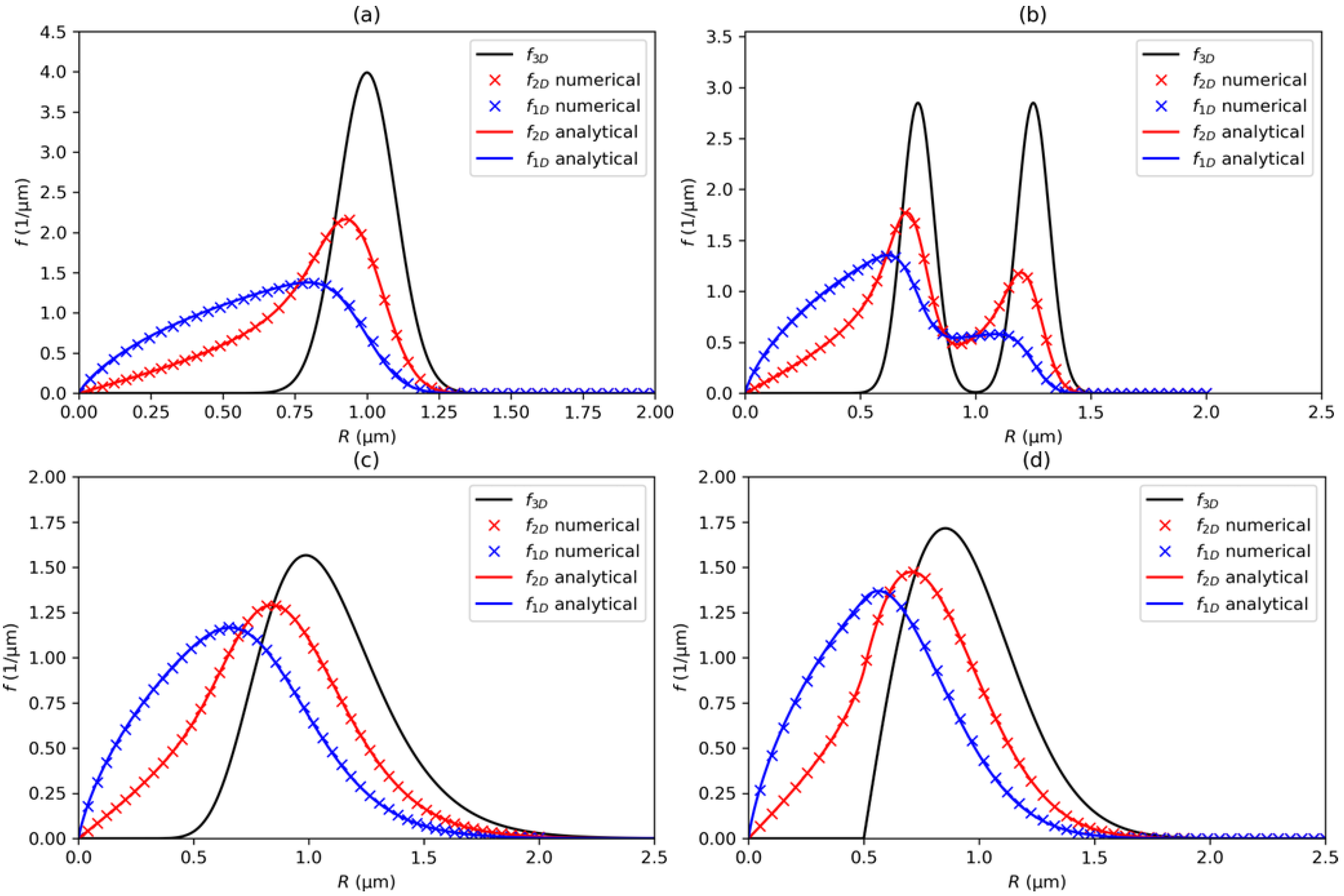
Crystals 13 00464 g003
Figure 4. Comparison of the numerical and analytical 2D and 1D distributions of the radii of cross-sections and linear intercepts considering (a) a normal distribution, (b) a bimodal distribution, (c) a log-normal distribution, and (d) a Weibull distribution. The 3D distribution is shown in the solid black line. The numerically generated 2D and 1D distribution functions are shown in the red and blue crosses, respectively.
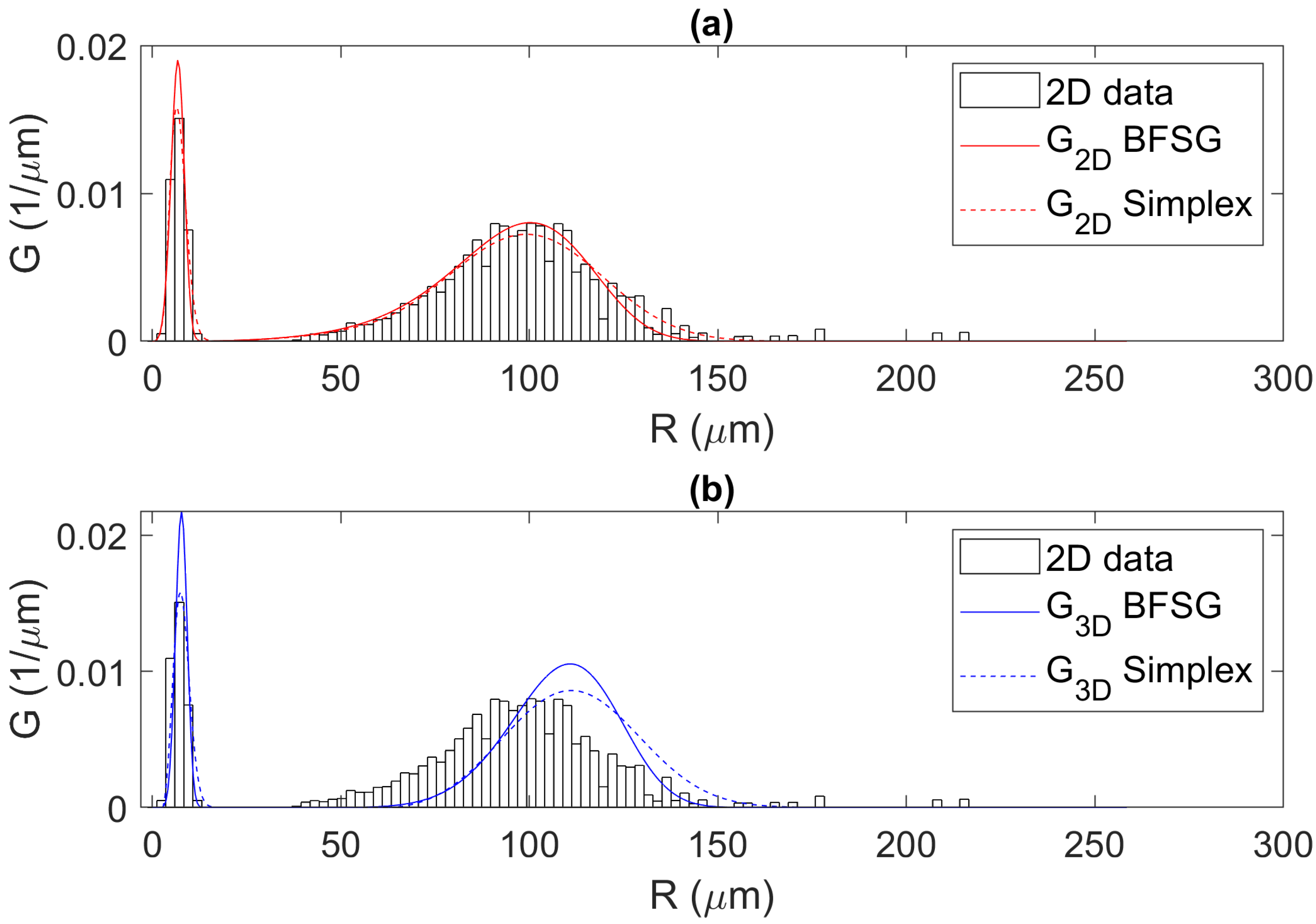
Crystals 13 00464 g004
Figure 5. Example applications of the inverse analysis of the 3D size of the particle distribution, considering (a) the γ distribution in CC IN738LC aged at 900 C for 10,000 h. (b) The primary γ in air quenched fine grain RR1000. (c,d) present the measured distribution of particle cross-sections compared with the approximated 3D and 2D distributions obtained using the BFSG algorithm and simplex method.
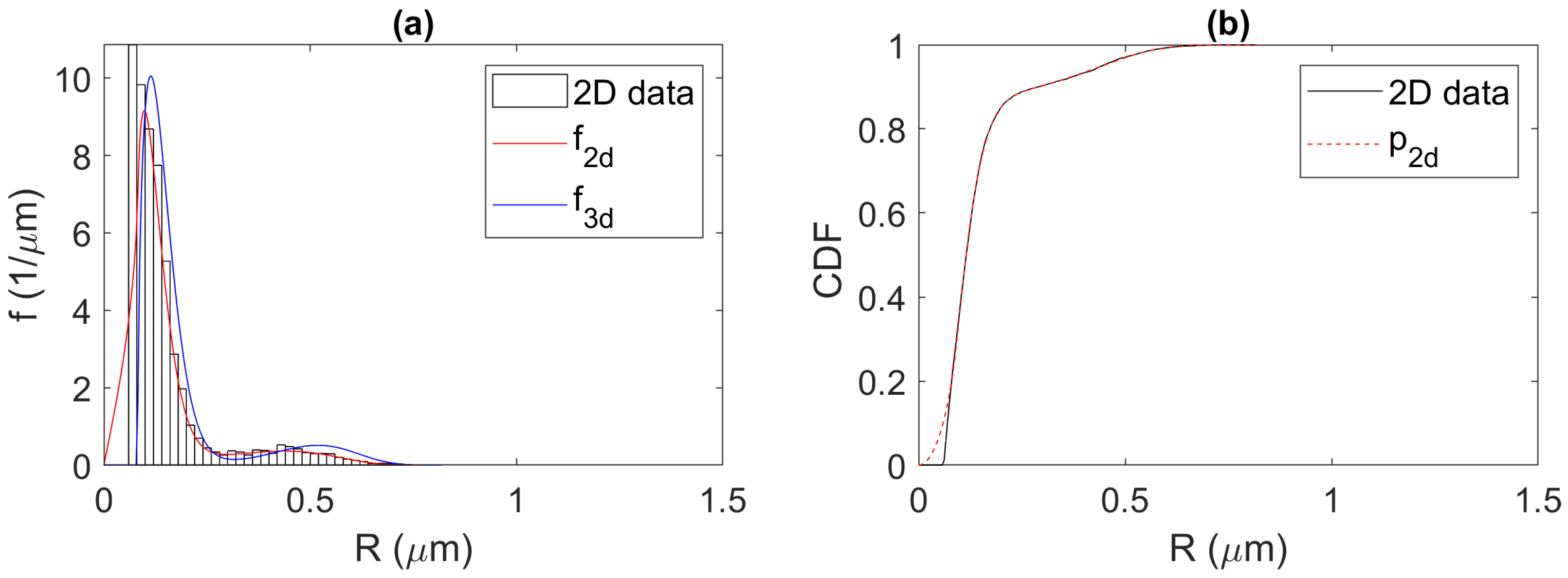
Crystals 13 00464 g005
Figure 6. (a) Comparison of the measured 2D data with the approximated 2D and 3D particle size distribution functions. The histogram presents the data, whilst the red and blue continuous lines describe the calculated 2D and 3D distribution functions. (b) The cumulative distribution functions comparing the 2D data and the 2D model, with the data described using the continuous black line, and the calculation in the dashed red line.
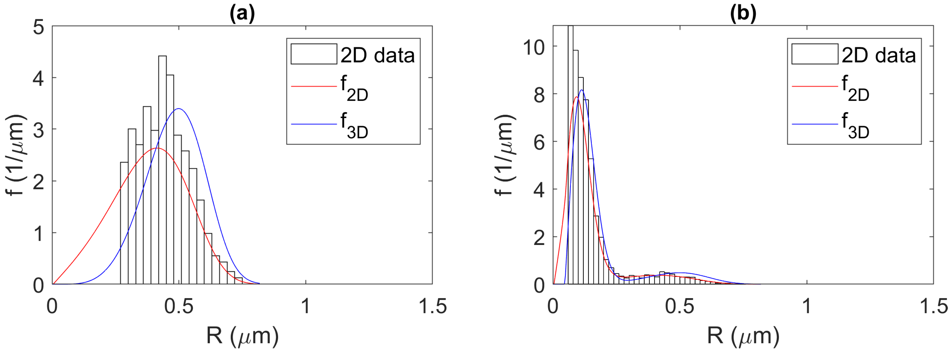
Crystals 13 00464 g006
Figure 7. (a) The comparison of the measured and calibrated probability size distribution functions, showing the 2D data, 2D prediction, and approximated 3D size distribution considering only the primary particles. (b) The comparison of the measured and calibrated probability size distribution functions for both primary and secondary populations.
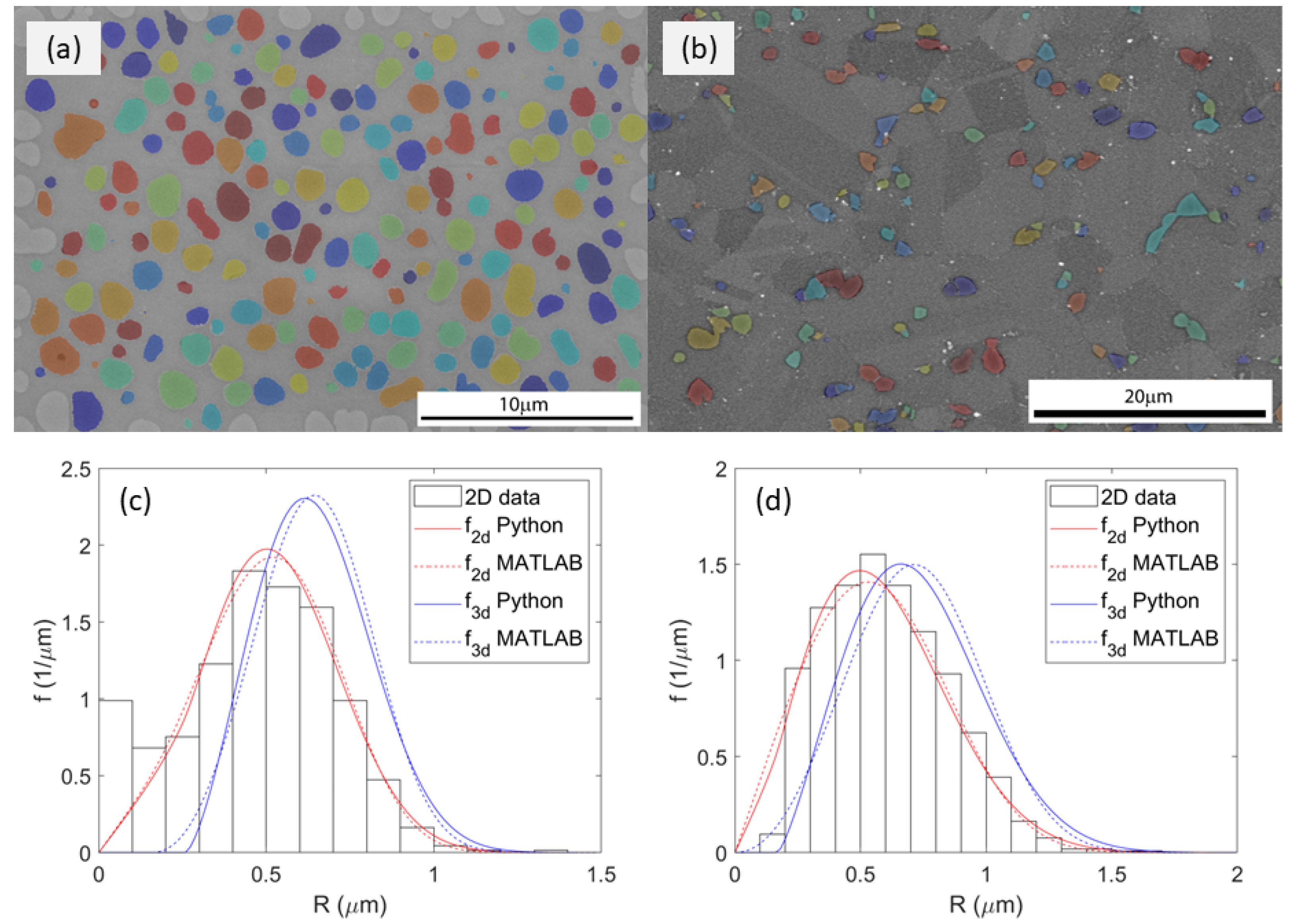
Crystals 13 00464 g007
Figure 8. The results from the inverse analysis of the bimodal γ size distribution in as-heat-treated coarse grain RR1000, comparing the simplex and BFSG methods. (a) presents the measured 2D distribution of particle cross-sections compared with calibrated 2D approximations of the data obtained from a Python and MATLAB implementation. (b) presents the approximated 3D size distributions in comparison to the measured 2D data.
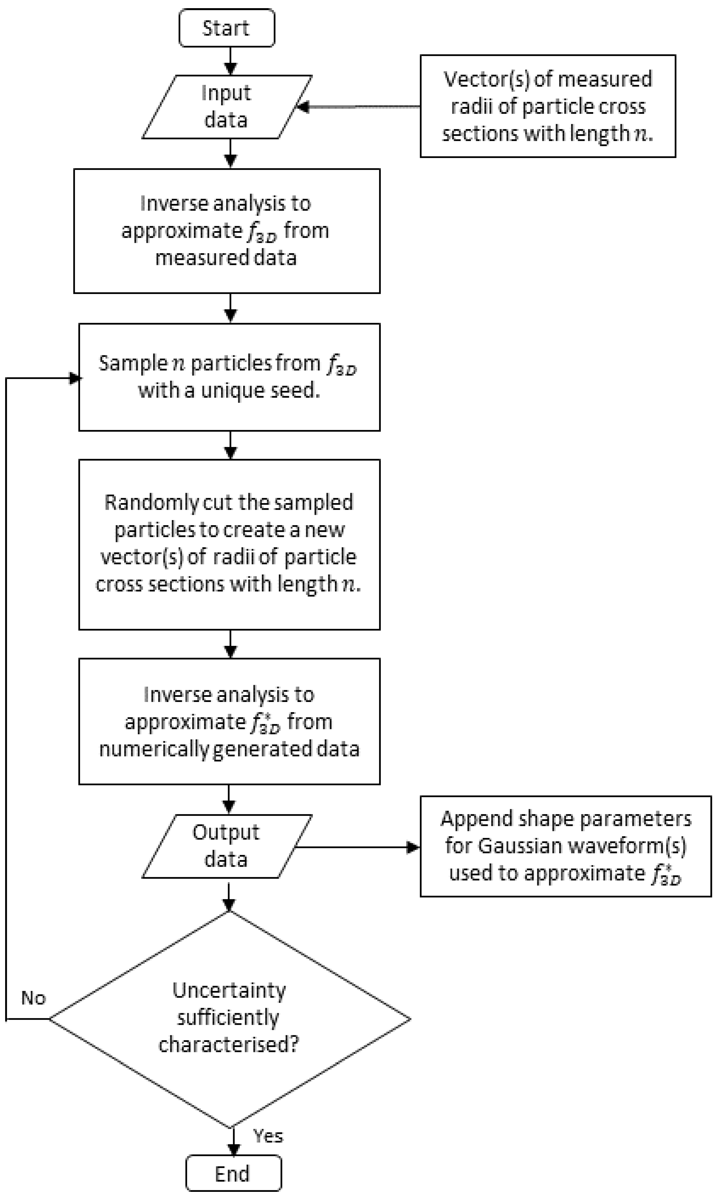
Crystals 13 00464 g008
Figure 9. A flowchart for uncertainty quantification when approximating the 3D size distribution from cross-sectional data.
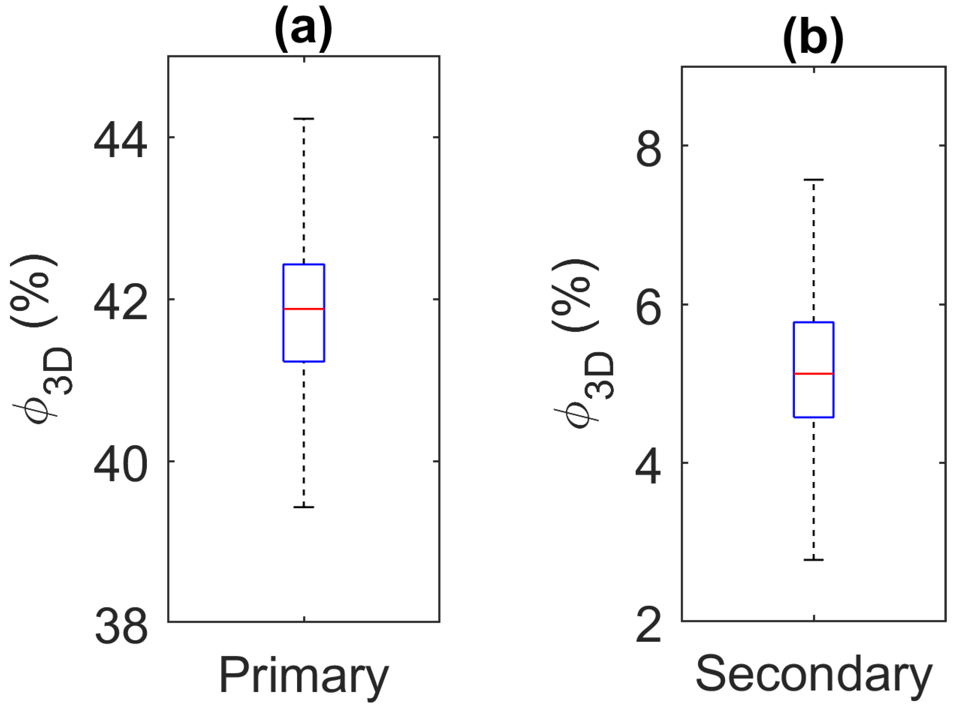
Crystals 13 00464 g009
Figure 10. Boxplots show the scatter in the predicted volume fraction of the (a) primary and (b) secondary particle populations considering a total of 2748 particle measurements.
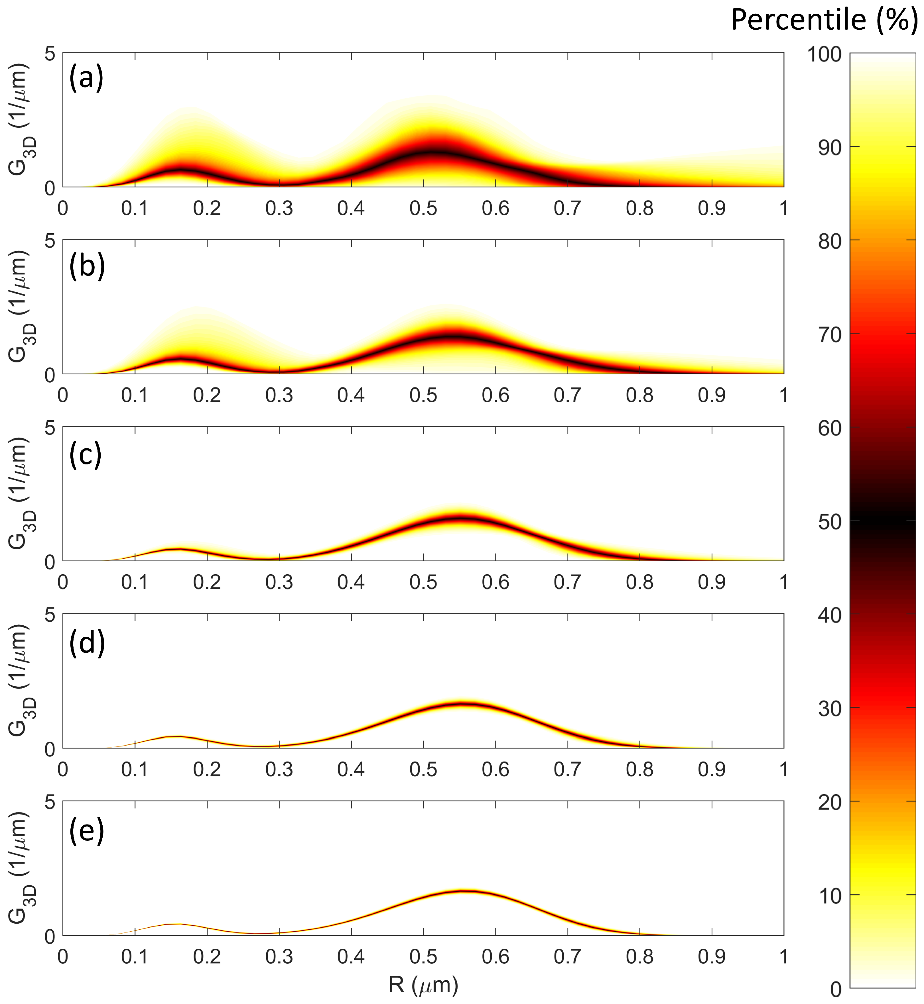
Crystals 13 00464 g010
Figure 11. The error and Uncertainty in the approximated 3D size distribution as a function of sample size, where (a) has a sample size of 300, (b) has 1000, (c), has 3000, (d) has 10,000, and (e) has a sample size of 30,000.
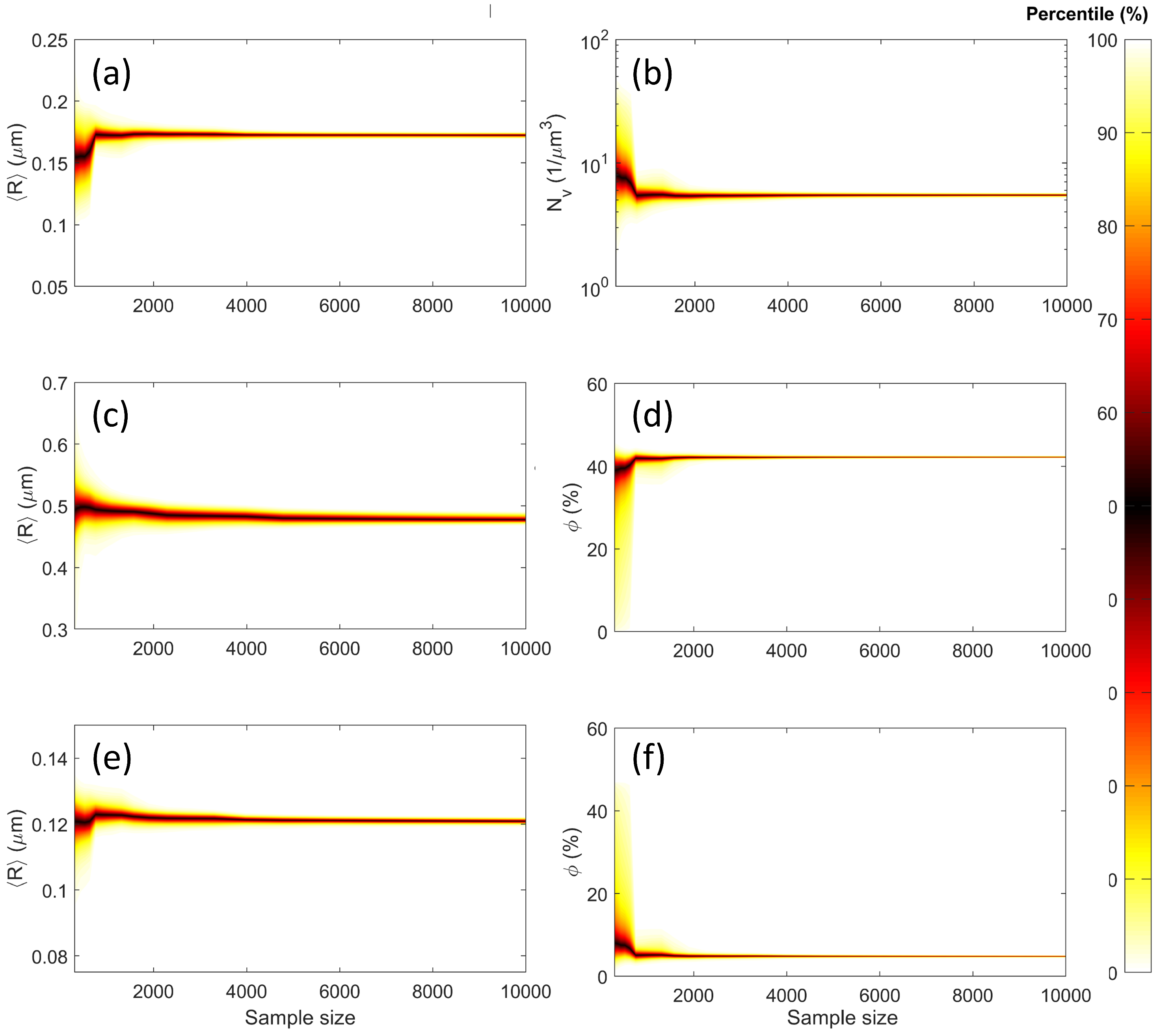
Crystals 13 00464 g011
Figure 12. Variation in predicted particle statistics as a function of sample size. (a,b) show the variation in percentiles for the mean particle radius and particle concentration considering the entire dispersion. (c,d) compare the mean particle radius and particle volume fraction for the primary particles, whilst (e,f) show the variation in mean particle radius and volume fraction for the secondary particles.
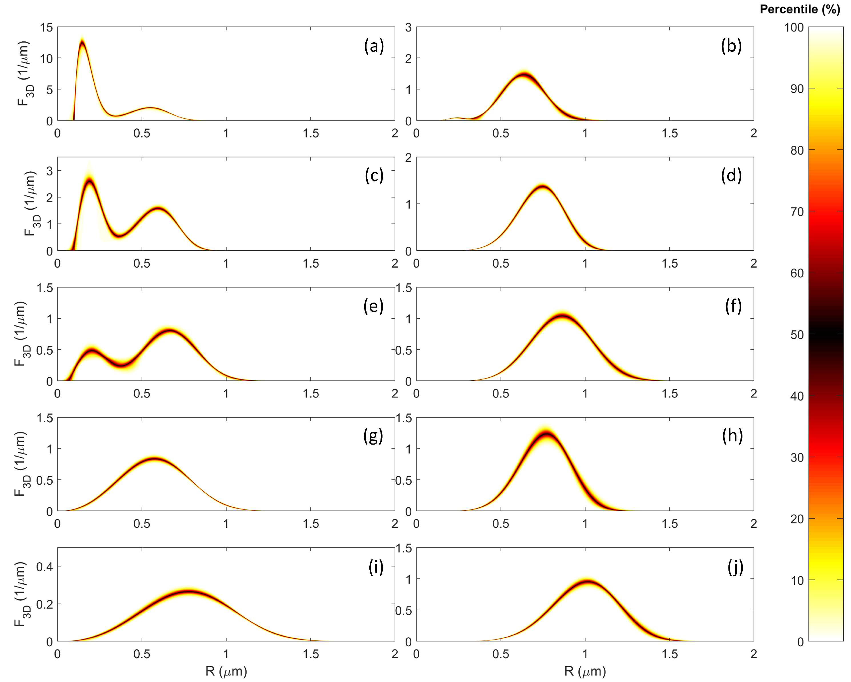
Crystals 13 00464 g012
Figure 13. The scatter and variation in approximated 3D particle size distributions in γ precipitates in IN738LC, aged at 850 °C and 900 °C for 1000 h, 2000 h, 3000 h, 10,000 h, and 20,000 h. (a,c,e,g,i) show the results from aging at 850 °C whilst figures (b,d,f,h,j) show the results from aging at 900 °C. (a,b) refer to aging times of 1000 h, (c,d) to 2000 h, (e,f) for 3000 h, (g,h) to 10,000 h, and (i,j) to 20,000 h.
Crystals 13 00464 g013
Table 1. This table lists the Gaussian waveforms used to assess the 3D → 2D conversion functions.
Gaussian Waveforms
(a) Normal unimodal
f 3 D ( R ) = 1 σ 2 π e x p R μ 2 2 σ 2
(25)
(b) Normal bimodal
f 3 D ( R ) = ζ σ 1 2 π e x p R μ 1 2 2 σ 1 2 + 1 ζ σ 2 2 π e x p R μ 2 2 2 σ 2 2
(26)
(c) Log-normal
f 3 D ( R ) = 1 σ 2 π R e x p 1 2 l n ( R ) μ σ 2
(27)
(d) Weibull
f 3 D = α β R γ β α 1 e x p R γ β α
(28)
Table 2. The parameters to generate different shapes of particle size distributions, corresponding to the waveforms presented in Table 1.
Distribution Type μ ( μ m) σ ( μ m) ζ γ ( μ m) α β ( μ m)
(a) Normal-unimodal10.1----
(b) Normal-bimodal0.75, 1.250.07, 0.250.5---
(c) Lognormal0.050.25----
(d) Weibull---0.530.5
Disclaimer/Publisher’s Note: The statements, opinions and data contained in all publications are solely those of the individual author(s) and contributor(s) and not of MDPI and/or the editor(s). MDPI and/or the editor(s) disclaim responsibility for any injury to people or property resulting from any ideas, methods, instructions or products referred to in the content.

