

Heterogeneous Substrates Modify Non-Classical Nucleation Pathways: Reanalysis of Kinetic Data from the Electrodeposition of Mercury on Platinum Using Hierarchy of Sigmoid Growth Models
 , and
, and
Abstract
:1. Introduction
2. Hierarchy of Models (HoM)
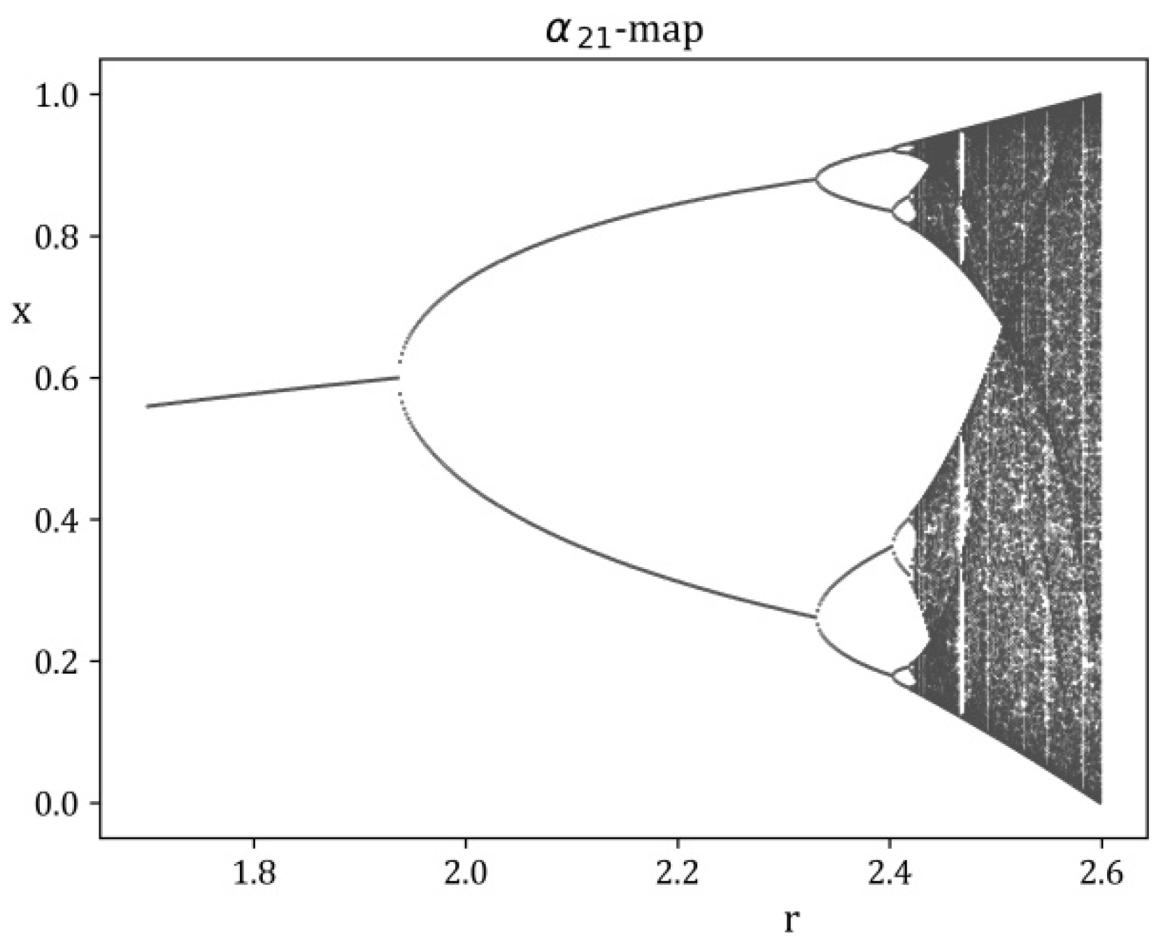
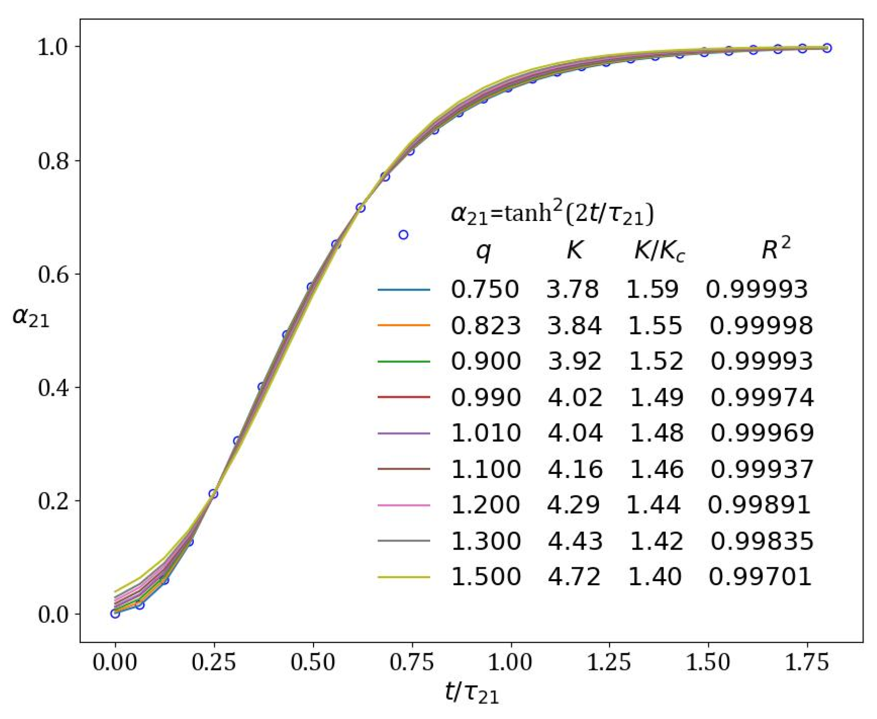
2.1. The α21 Model [6]
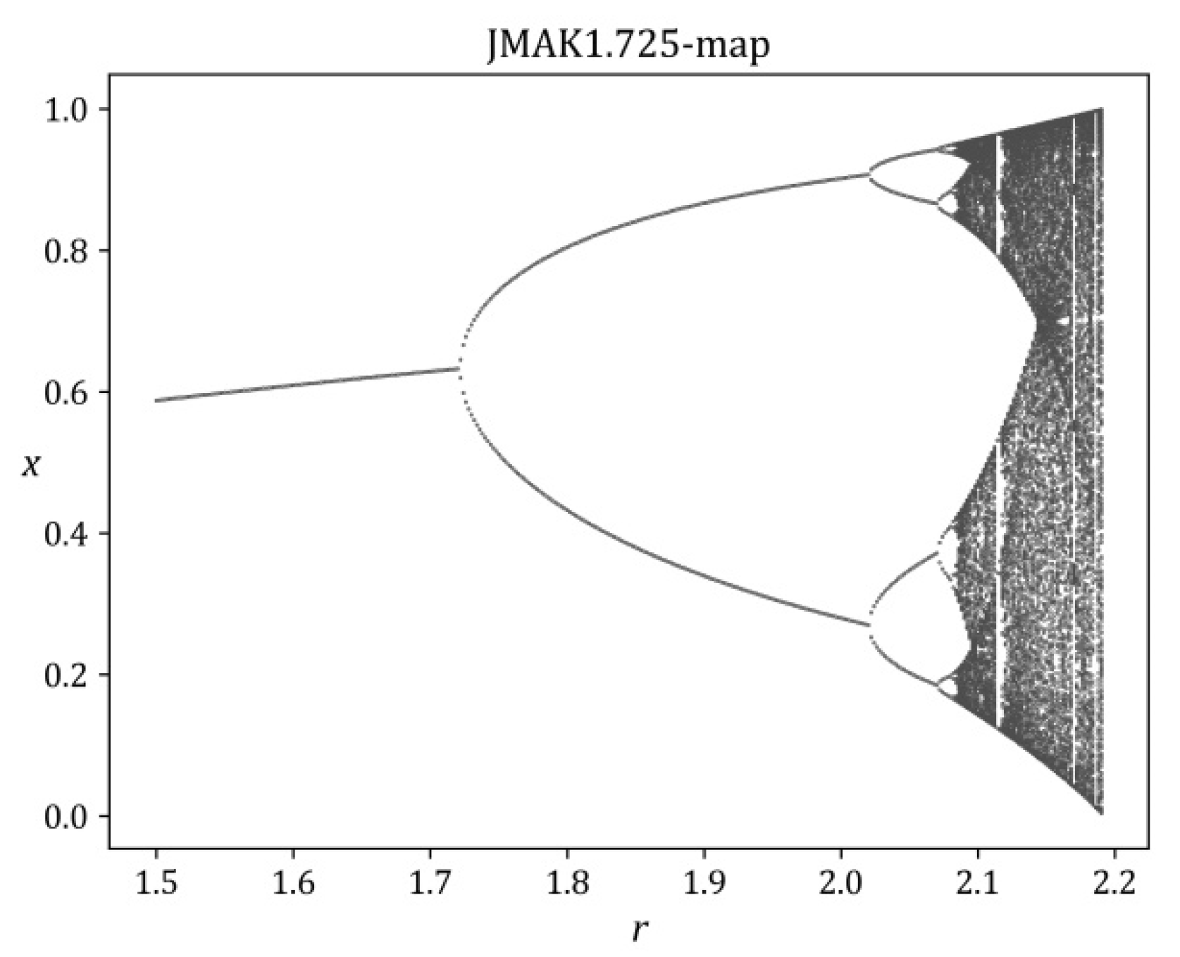
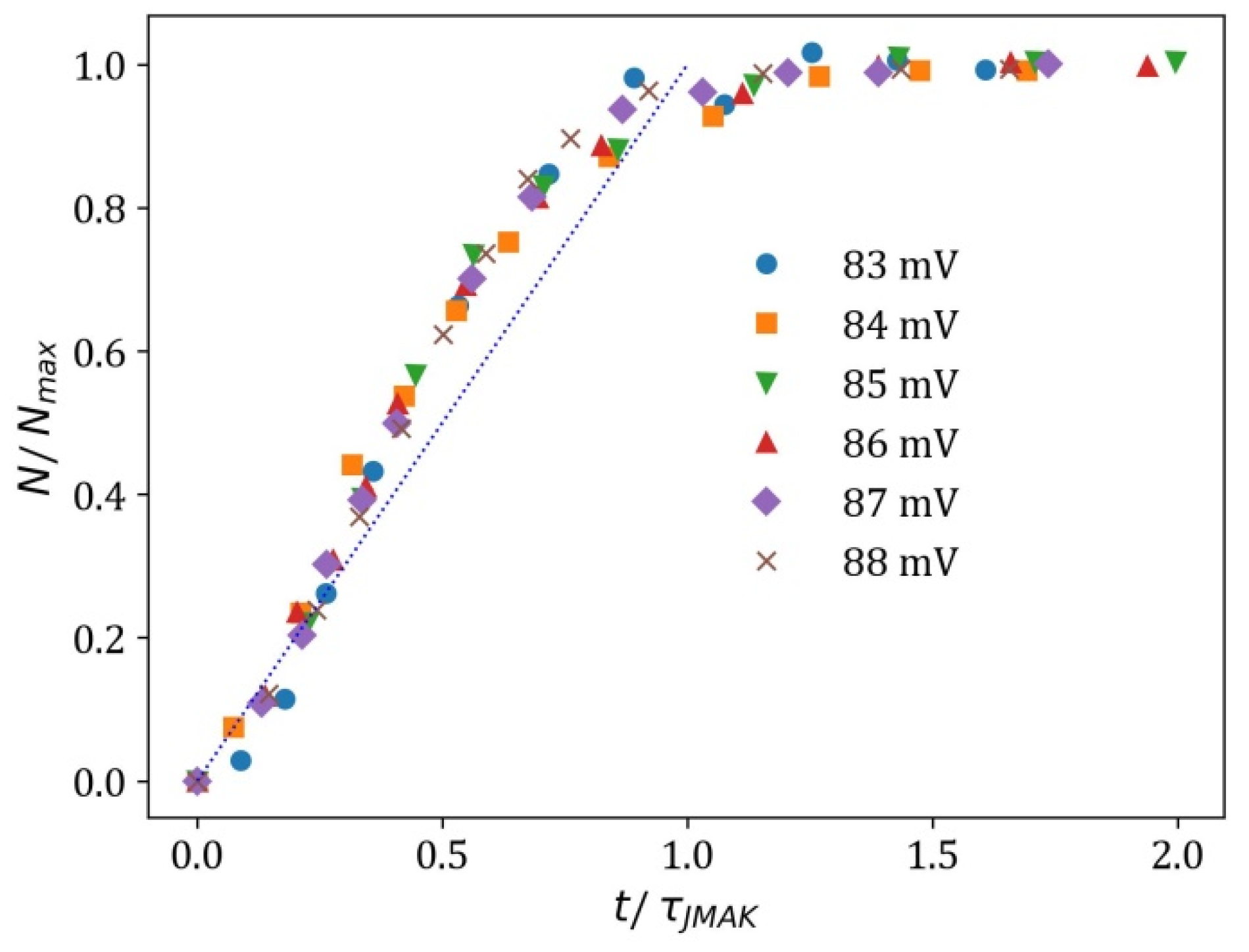
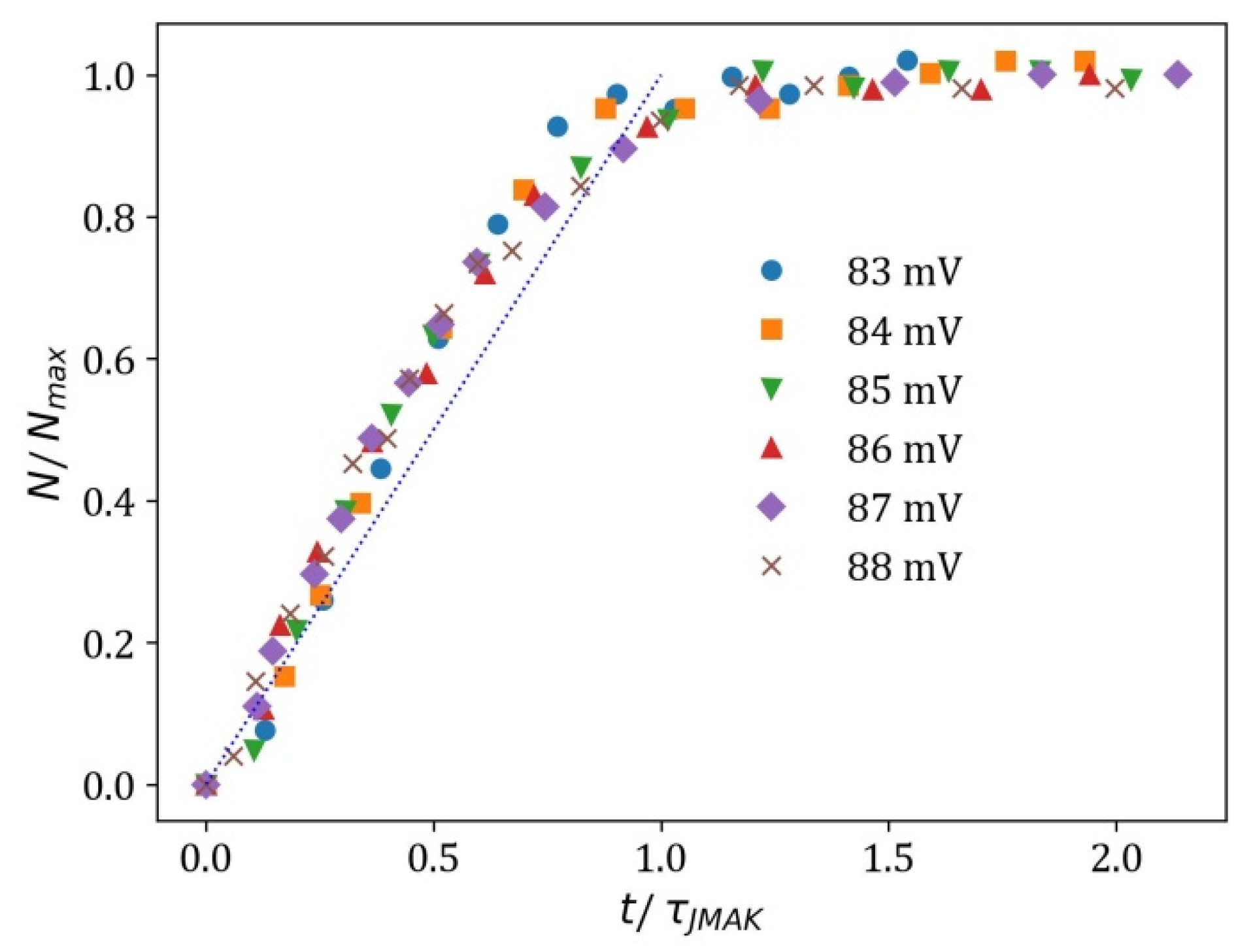
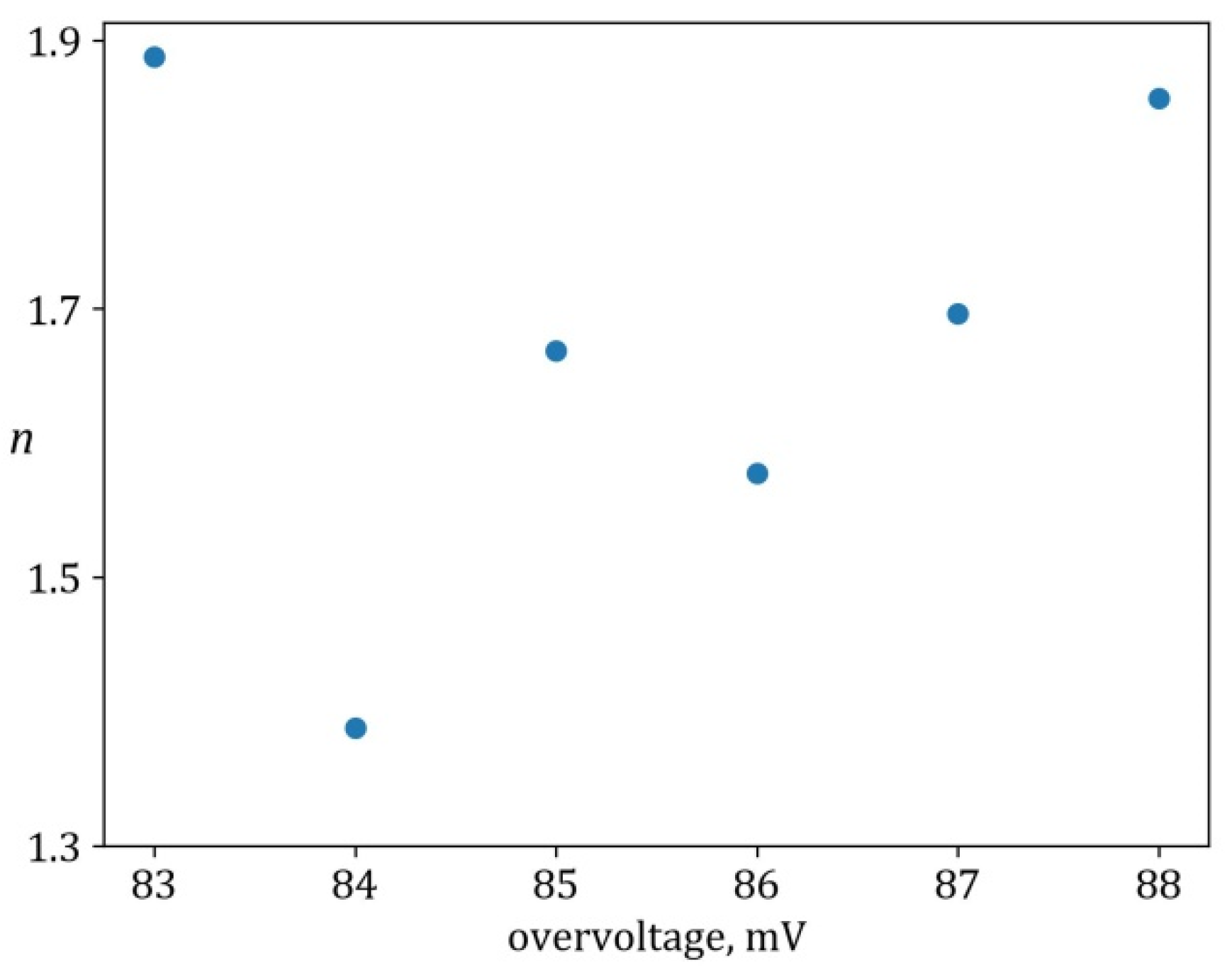
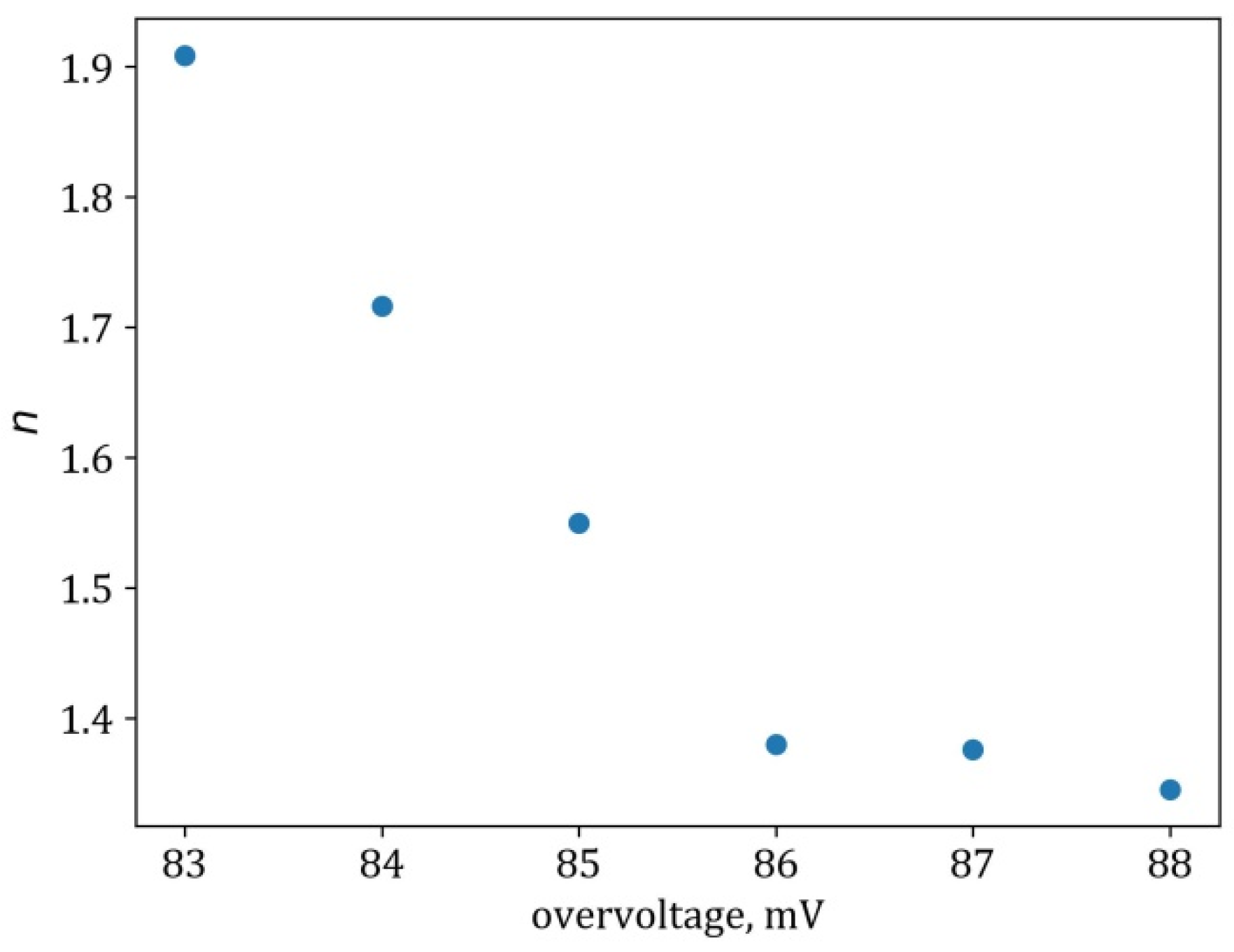
2.2. The Johnson–Mehl–Avrami–Kolmogorov Model (JMAKn)
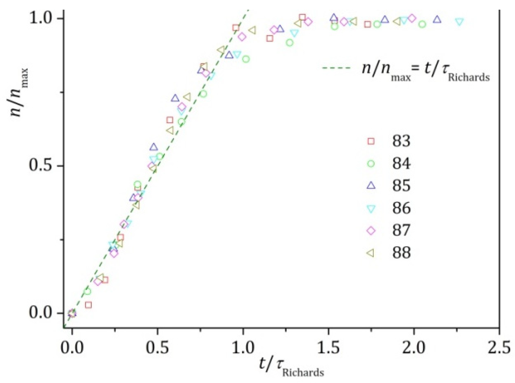
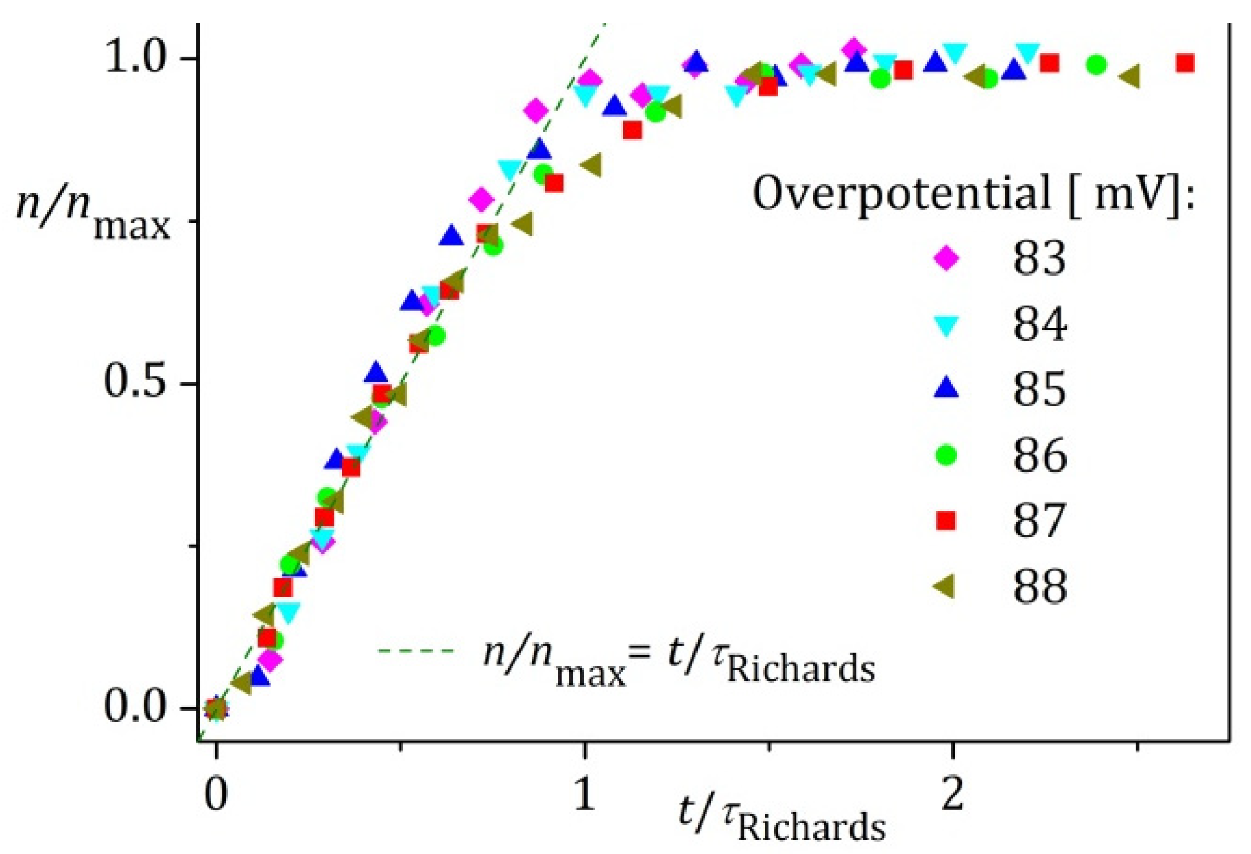
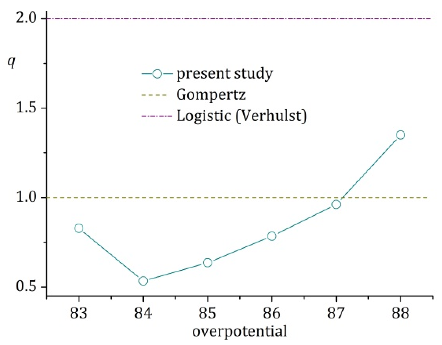
2.3. Richards Model
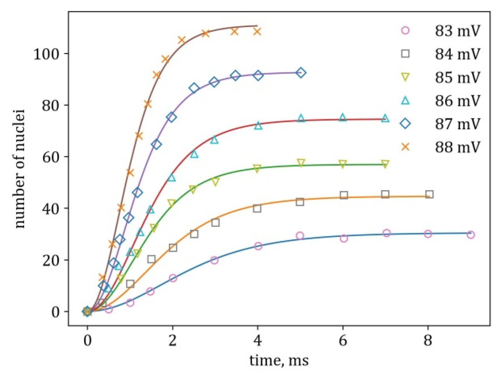
3. Results
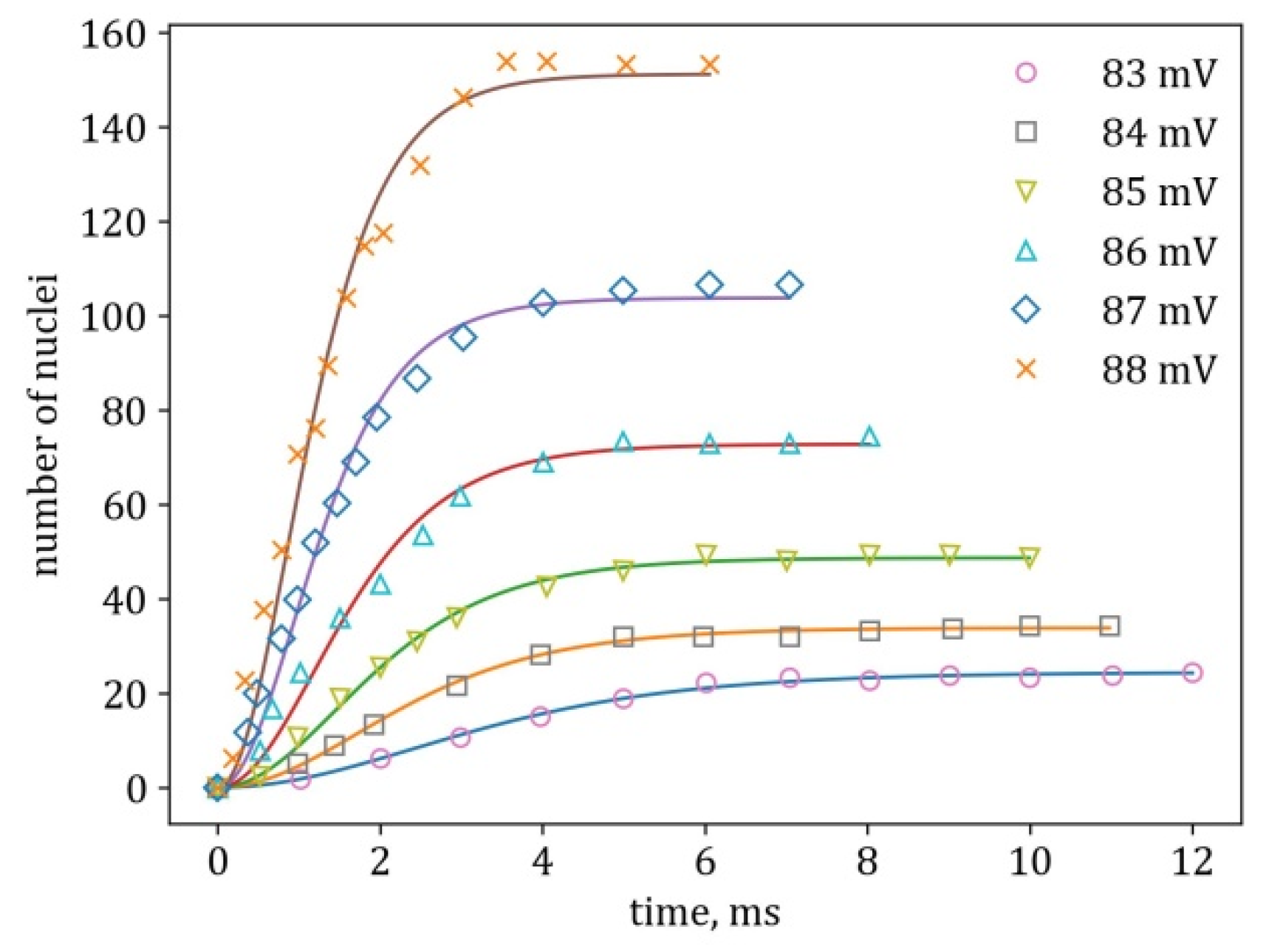
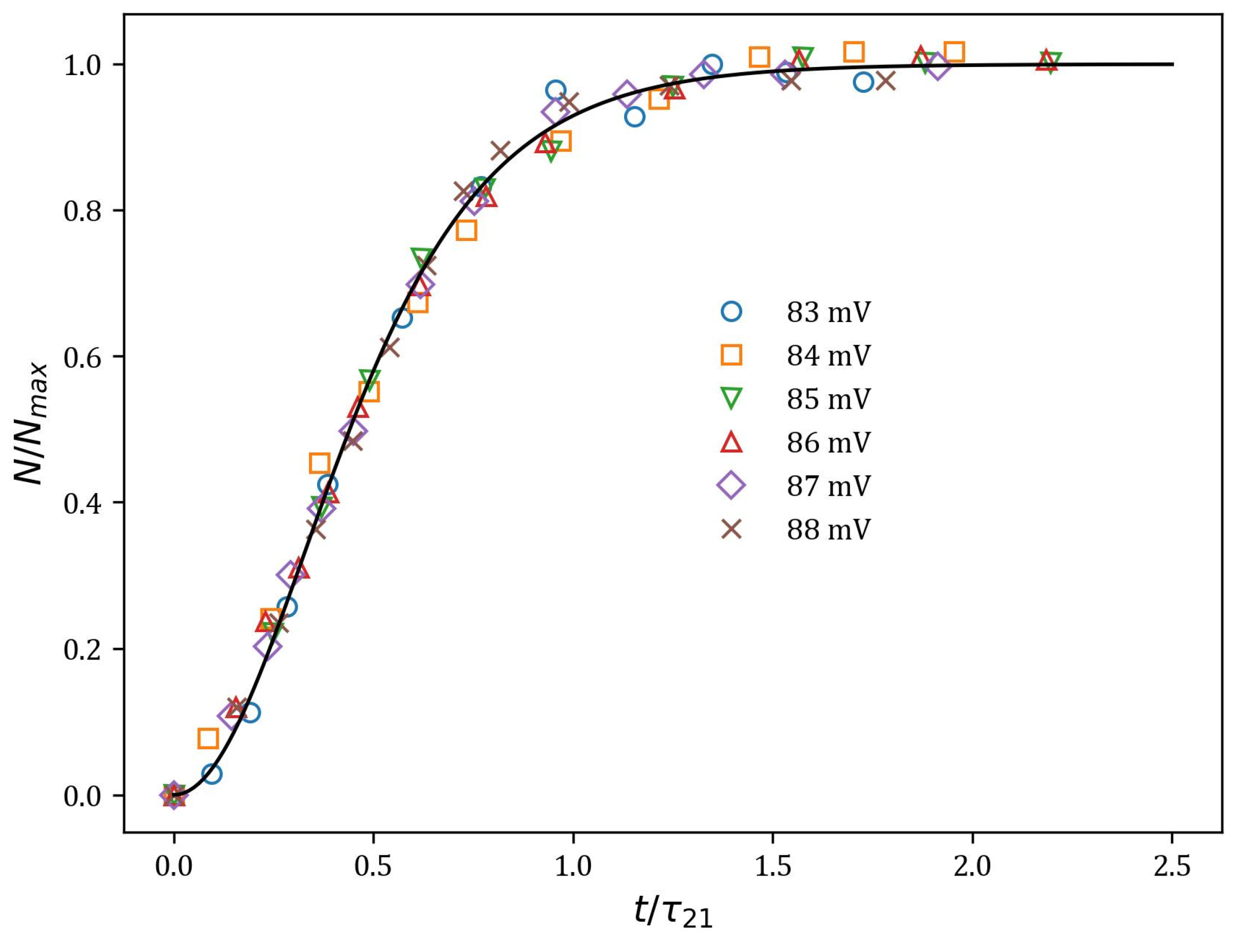
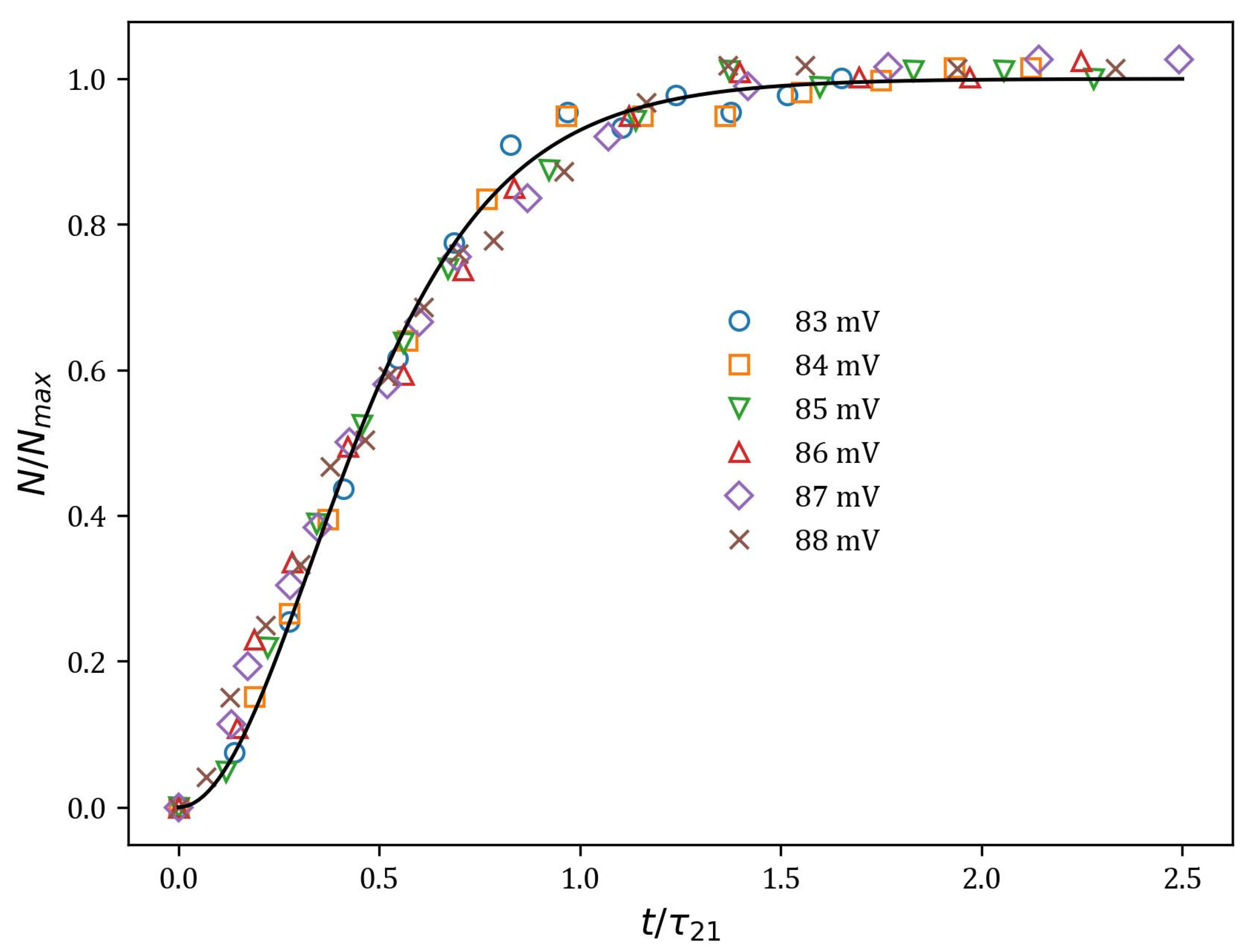
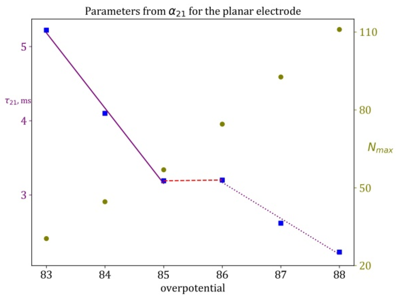
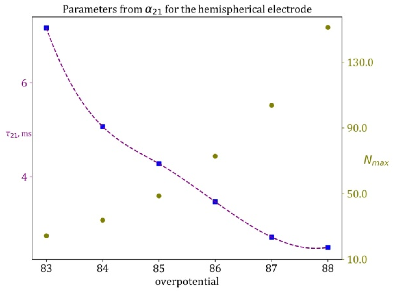
3.1. Fitting with the α21 Model
3.2. Summary of the Fitting Procedure
4. Discussion and Conclusions
Author Contributions
Funding
Data Availability Statement
Acknowledgments
Conflicts of Interest
Appendix A
Appendix A.1. Fitting with the JMAKn Model


Appendix A.2. Fitting with the Richards Model


References
- Markov, I.; Stoycheva, E. Saturation Nucleus Density in the Electrodeposition of Metals onto Inert Electrodes II. Experimental. Thin Solid Film. 1976, 21, 35. [Google Scholar] [CrossRef]
- Budevski, E.; Staikov, G.; Lorenz, W. Electrocrystallization: Nucleation and Growth Phenomena. Electrochim. Acta 2000, 2559, 45. [Google Scholar]
- Milchev, A. Nucleation Phenomena in Electrochemical Systems: Kinetic Models. ChemTexts 2016, 4, 2. [Google Scholar] [CrossRef]
- Popov, K.I.; Djokić, S.S.; Nikolić, N.D.; Jović, V.D. Morphology of Electrochemically and Chemically Deposited Metals; Springer: Berlin/Heidelberg, Germany, 2016. [Google Scholar]
- Milchev, A. Thermodynamics of Electrochemical Nucleation; Springer: Berlin/Heidelberg, Germany, 2002. [Google Scholar]
- Ivanov, V.V.; Tielemann, C.; Avramova, K.; Reinsch, S.; Tonchev, V. Modelling Crystallization: When the Normal Growth Velocity Depends on the Supersaturation. J. Phys. Chem. Solids 2023, 111542, 181. [Google Scholar] [CrossRef]
- Vekilov, P.G. The Two-Step Mechanism of Nucleation of Crystals in Solution. Nanoscale 2010, 2346, 2. [Google Scholar] [CrossRef] [PubMed]
- Nanev, C.N.; Tonchev, V.D. Sigmoid Kinetics of Protein Crystal Nucleation. J. Cryst. Growth 2015, 48, 427. [Google Scholar] [CrossRef]
- Verhulst, P.-F. Notice Sur La Loi Que La Population Suit Dans Son Accroissement. Corresp. Math. Phys. 1838, 113, 10. [Google Scholar]
- Tjørve, E.; Tjørve, K.M. A Unified Approach to the Richards-Model Family for Use in Growth Analyses: Why We Need Only Two Model Forms. J. Theor. Biol. 2010, 417, 267. [Google Scholar] [CrossRef]
- Watzky, M.A.; Finke, R.G. Transition Metal Nanocluster Formation Kinetic and Mechanistic Studies. A New Mechanism When Hydrogen Is the Reductant: Slow, Continuous Nucleation and Fast Autocatalytic Surface Growth. J. Am. Chem. Soc. 1997, 10382, 119. [Google Scholar] [CrossRef]
- Bentea, L.; Watzky, M.A.; Finke, R.G. Sigmoidal Nucleation and Growth Curves across Nature Fit by the Finke–Watzky Model of Slow Continuous Nucleation and Autocatalytic Growth: Explicit Formulas for the Lag and Growth Times plus Other Key Insights. J. Phys. Chem. C 2017, 5302, 121. [Google Scholar] [CrossRef]
- Barlow, D.A. The Kinetics of Multi-Step Protein Crystal Growth from Solution. Horiz. World Phys. 2021, 306, 151–186. [Google Scholar]
- Barlow, D.; Gregus, J. The Kinetics of Homogeneous and Two-Step Nucleation during Protein Crystal Growth from Solution. Int. J. Chem. Kinet. 2019, 840, 51. [Google Scholar] [CrossRef]
- Nanev, C.N.; Tonchev, V.D.; Hodzhaoglu, F.V. Protocol for Growing Insulin Crystals of Uniform Size. J. Cryst. Growth 2013, 10, 375. [Google Scholar] [CrossRef]
- Kleshtanova, V.; Tonchev, V.; Stoycheva, A.; Angelov, C. Cloud Condensation Nuclei and Backward Trajectories of Air Masses at Mt. Moussala in Two Months of 2016. J. Atmos. Sol.-Terr. Phys. 2023, 106004, 243. [Google Scholar] [CrossRef]
- Kolmogorov, A.N. On the Statistical Theory of the Crystallization of Metals. Bull. Acad. Sci. USSR Math. Ser. 1937, 355, 1. [Google Scholar]
- Johnson, W.; Mehl, R. Reaction kinetics in processes of nucleation and growth. Trans. Metall. Soc. AIME 1939, 135, 416–442. [Google Scholar]
- Avrami, M. Kinetics of Phase Change. I General Theory. J. Chem. Phys. 1939, 1103, 7. [Google Scholar] [CrossRef]
- Málek, J. Kinetic Analysis of Crystallization Processes in Amorphous Materials. Thermochim. Acta 2000, 239, 355. [Google Scholar] [CrossRef]
- Avramov, I. Kinetics of Distribution of Infections in Networks. Phys. A Stat. Mech. Its Appl. 2007, 615, 379. [Google Scholar] [CrossRef]
- Dill, E.D.; Folmer, J.C.; Martin, J.D. Crystal Growth Simulations to Establish Physically Relevant Kinetic Parameters from the Empirical Kolmogorov–Johnson–Mehl–Avrami Model. Chem. Mater. 2013, 3941, 25. [Google Scholar] [CrossRef]
- Shirzad, K.; Viney, C. A Critical Review on Applications of the Avrami Equation beyond Materials Science. J. R. Soc. Interface 2023, 20, 20230242. [Google Scholar] [CrossRef] [PubMed]
- Gompertz, B. XXIV. On the Nature of the Function Expressive of the Law of Human Mortality, and on a New Mode of Determining the Value of Life Contingencies. In a Letter to Francis Baily, Esq. FRS &c; Philosophical Transactions of the Royal Society of London: London, UK, 1825; Volume 513. [Google Scholar]
- Zeeman, E.C. Catastrophe Theory, in Structural Stability in Physics: Proceedings of Two International Symposia on Applications of Catastrophe Theory and Topological Concepts in Physics Tübingen, Fed. Rep. of Germany, May 2–6 and December 11–14, 1978; Springer: Berlin/Heidelberg, Germany, 1979; pp. 12–22. [Google Scholar]
- Markov, I. Saturation Nucleus Density in the Electrodeposition of Metals onto Inert Electrodes I. Theory. Thin Solid Films 1976, 11, 35. [Google Scholar]
- Markov, I.V. Crystal Growth for Beginners: Fundamentals of Nucleation, Crystal Growth and Epitaxy; World Scientific: Singapore, 2016. [Google Scholar]
- Markov, I.V. Ivan Stranski—The Grandmaster of Crystal Growth; World Scientific: Singapore, 2019. [Google Scholar]


| Over-Voltage, mV | α21 | JMAKn | Richards | ||||||||
|---|---|---|---|---|---|---|---|---|---|---|---|
| Nmax | τ21 | R2 | Nmax | τJMAK | n | R2 | Nmax | τR | q | R2 | |
| 83 | 30.43 | 5.22 | 0.9974 | 29.9 | 5.6 | 1.89 | 0.9977 | 30.29 | 5.20 | 0.83 | 0.9967 |
| 84 | 44.61 | 4.11 | 0.9937 | 45.78 | 4.75 | 1.39 | 0.9986 | 46.28 | 3.93 | 0.53 | 0.9981 |
| 85 | 56.94 | 3.19 | 0.9986 | 56.86 | 3.51 | 1.67 | 0.9980 | 57.36 | 3.28 | 0.64 | 0.9984 |
| 86 | 74.51 | 3.20 | 0.9976 | 75.06 | 3.61 | 1.58 | 0.9992 | 75.60 | 3.09 | 0.79 | 0.9988 |
| 87 | 92.7 | 2.62 | 0.9988 | 92.37 | 2.89 | 1.70 | 0.9995 | 93.17 | 2.52 | 0.96 | 0.9989 |
| 88 | 111.01 | 2.23 | 0.9974 | 109.19 | 2.40 | 1.86 | 0.9990 | 109.57 | 2.09 | 1.35 | 0.9983 |
| Over-Voltage, mV | α21 | JMAKn | Richards | ||||||||
|---|---|---|---|---|---|---|---|---|---|---|---|
| nmax | τ21 | R2 | Nmax | τJMAK | n | R2 | nmax | τR | q | R2 | |
| 83 | 24.41 | 7.27 | 0.9966 | 23.92 | 7.79 | 1.91 | 0.9978 | 24.12 | 6.95 | 1.18 | 0.9963 |
| 84 | 33.84 | 5.17 | 0.9977 | 33.68 | 5.69 | 1.72 | 0.9978 | 33.93 | 4.98 | 0.93 | 0.9971 |
| 85 | 48.69 | 4.38 | 0.9969 | 48.97 | 4.92 | 1.55 | 0.9985 | 48.19 | 4.62 | 0.43 | 0.9987 |
| 86 | 72.78 | 3.57 | 0.9890 | 74.50 | 4.13 | 1.38 | 0.9967 | 73.07 | 3.36 | 0.51 | 0.9948 |
| 87 | 103.77 | 2.82 | 0.9923 | 106.51 | 3.30 | 1.38 | 0.9993 | 103.81 | 2.68 | 0.54 | 0.9990 |
| 88 | 151.22 | 2.60 | 0.9891 | 156.27 | 3.03 | 1.35 | 0.9971 | 151.30 | 2.43 | 0.52 | 0.9958 |
Disclaimer/Publisher’s Note: The statements, opinions and data contained in all publications are solely those of the individual author(s) and contributor(s) and not of MDPI and/or the editor(s). MDPI and/or the editor(s) disclaim responsibility for any injury to people or property resulting from any ideas, methods, instructions or products referred to in the content. |
© 2023 by the authors. Licensee MDPI, Basel, Switzerland. This article is an open access article distributed under the terms and conditions of the Creative Commons Attribution (CC BY) license (https://creativecommons.org/licenses/by/4.0/).
Share and Cite
Kleshtanova, V.; Ivanov, V.V.; Hodzhaoglu, F.; Prieto, J.E.; Tonchev, V. Heterogeneous Substrates Modify Non-Classical Nucleation Pathways: Reanalysis of Kinetic Data from the Electrodeposition of Mercury on Platinum Using Hierarchy of Sigmoid Growth Models. Crystals 2023, 13, 1690. https://doi.org/10.3390/cryst13121690
Kleshtanova V, Ivanov VV, Hodzhaoglu F, Prieto JE, Tonchev V. Heterogeneous Substrates Modify Non-Classical Nucleation Pathways: Reanalysis of Kinetic Data from the Electrodeposition of Mercury on Platinum Using Hierarchy of Sigmoid Growth Models. Crystals. 2023; 13(12):1690. https://doi.org/10.3390/cryst13121690
Chicago/Turabian StyleKleshtanova, Viktoria, Vassil V. Ivanov, Feyzim Hodzhaoglu, Jose Emilio Prieto, and Vesselin Tonchev. 2023. "Heterogeneous Substrates Modify Non-Classical Nucleation Pathways: Reanalysis of Kinetic Data from the Electrodeposition of Mercury on Platinum Using Hierarchy of Sigmoid Growth Models" Crystals 13, no. 12: 1690. https://doi.org/10.3390/cryst13121690