A Least Squares Fitting Method for Uncertain Parameter Estimation in Solidification Model

Abstract

This study proposes an automated method for estimating the uncertain parameters of the solidification model in response to the inefficient and time-consuming problem of manually estimating multiple uncertain parameters of the solidification model. The method establishes an uncertain parameter estimation model based on the relationship between the simulated images equiaxed crystal ratio and the uncertain parameters of the solidification model, fits the parameters of the model by the least squares method, and finally estimates the uncertain parameters in the solidification model using the parameters of the fitted model. In comparison with the traditional method of calculating uncertain parameters manually through empirical formulas, this method reduces the difficulty of tuning parameters and solves the problem of tuning multiple parameters simultaneously in the nonlinear solidification model. The experimental results show that the proposed method can accurately estimate the uncertain parameters of the solidification model, improve the efficiency and accuracy of the solidification model estimation parameters, and play a guiding role in simulating the solidification process of continuously casting billet to control the solidification structure.

1. Introduction

The iron and steel industry is an important industry in the foundation of the national economy and an important area for realising green and low-carbon development. More than 80% of the world’s casting process is related to the continuous casting process, and the steel industry every year suffers losses amounting to hundreds of millions of dollars due to billet quality problems, causing direct economic losses. Therefore, billet quality detection is one of the important problems in the steel industry. The solidification structure reflects the quality of the cast billet [1,2,3], and the macroscopic solidification structure of the cast billet usually consists of three parts: fine equiaxed crystals on the surface, columnar crystals, and central equiaxed crystals. The equiaxed crystal ratio is one of the important indicators of the quality of cast billet [4,5], and it is usually hoped to obtain a large equiaxed crystal ratio of cast billet except for in some special-purpose steel grades that require a columnar crystal structure. The larger the equiaxed crystal ratio of the cast billet, the better the stability of the cast billet [6]. Several researchers have used numerical simulation methods such as phase field models [7,8,9,10] and metameric automata models [11,12,13] to study the structure changes during metal solidification [14,15,16,17] for controlling the quality of cast billets. Ideally, the simulated image should be consistent with the solidification organization of the actual as-cast image, but in the practical situation, there are often some differences between the simulated image and the actual low-magnification specimen, as shown in Figure 1. Improvement of solidification modelling accuracy has become a key issue that needs to be solved [18,19,20].

Assuming that the established simulation solidification model is correct, the reason for the discrepancy is that the parameters in the solidification model are incorrect and need to be adjusted [21,22,23]. The traditional tuning method is to adjust the parameters according to the empirical formula, which has the following problems:

(1)

The solidification process of cast billet is complicated and affected by multiple physical fields and factors. The solidification model is nonlinear, and it is difficult to adjust the parameters;

(2)

There are many uncertain parameters in the solidification model, and the parameters affect each other. There is the problem of parameter redundancy, and all parameters cannot be determined at the same time.

To solve the above problems, an automatic estimation method of uncertain parameters of the solidification model for continuously casting billets is proposed based on the idea of inverse analysis of the solidification model. The solidification mechanism model has rigorous logic and derivation, and by inputting a set of model parameters, it can generate a low-magnification simulation image. According to the inverse analysis idea, it can recognize the equiaxed crystal ratio of the simulated image, analyse the relationship between the equiaxed crystal ratio and the solidification parameters, and establish a parameter estimation model to estimate the uncertain parameters.

Several researchers have also carried out studies using inverse analysis for parameter estimation. Natsume et al. [24] proposed a method to estimate the heat-transfer coefficient of alloys during solidification, which can accurately model the cooling curve of alloys during solidification. Drezet et al. [25] proposed an inversion method based on the MAP(Maximum A Posteriori) algorithm for the steady-state temperature field to study the effect of the parameter. Cheung et al. [26] studied the determination of transient metal/mould heat-transfer coefficients by describing an experimental set-up as part of a methodology linked to a numerical heat-transfer model that can be used to simulate solidification in industrial processes. Gao et al. [27] proposed a neural-network-based displacement inverse analysis method to identify the mechanical parameters of the surrounding rock.

The aim of the method in this paper is to establish the nonlinear mapping relationship between the uncertain parameters of the solidification model and the equiaxed crystal ratio to achieve the automatic estimation of the uncertain parameters, which can reduce lots of manual operations and provide a basis for verifying the accuracy of the solidification model. As the solidification of cast billets is affected by a variety of factors, and there are transitional mixed crystal regions between the columnar crystal regions in the equiaxed crystal region, there is no clear definition of the boundary between the various crystal regions [28,29], and the recognition results inevitably have some errors. This paper analyses the effect of the error on the estimated parameters by adding noise to the recognized equiaxed crystal ratio to simulate the recognition error.

2. Materials and Methods

2.1. Cellular Automaton (CA) Model

This paper investigates a solidification model based on a cellular automaton (CA) model to simulate the solidification of continuous billets. The CA method enables the evolution of a solidified structure by defining local transformation rules for nucleation and growth mechanisms [30]. In the CA method, each cell is divided into three states: liquid, interface, and solid. Using the continuous kernel model proposed by Thevoz et al. [31], the increment of the nucleation density is ${\mathrm{d}}_n$. The relationship between ${\mathrm{d}}_n$ and the undercooling at a given undercooling degree $\Delta T$ should follow a Gaussian distribution as shown in Equation (1):

$$\frac{{\mathrm{d}}_n}{d\left(\Delta T\right)}=\frac{n_{\max }}{\sqrt{2\pi }}\exp \left[-\frac{1}{2}{\left(\frac{\Delta T-\Delta T_n}{\Delta T_{\sigma }}\right)}^2\right]$$

(1)

where $\Delta T$ is the undercooling, $\Delta T_{\sigma }$ is the standard deviation, and $n_{\max }$ is maximum nucleation density. The $\Delta T_{\mathrm{n}}$ corresponds to the mean of the conventional Gaussian distribution, and $\Delta T_{\sigma }$ is equivalent to the variance of the conventional Gaussian distribution. $\Delta T_{\mathrm{n}}$, $\Delta T_{\sigma }$, and $n_{\max }$ are uncertain parameters of the solidification model and need to be estimated by subsequent modelling. The initial values of the nucleation parameters are shown in

Table 1. Table of initial values of nucleation parameters.

$n_{\max } \left(1/m^2\right)$	$\Delta T_{\mathrm{n}} \left(K\right)$	$\Delta T_{\sigma } \left(K\right)$
$2\times {10}^5$	12	1.5

.

The KGT [32] model is used to describe interfacial cell growth. Based on the theory of solute equilibrium at dendrite tips, the relationship between solute supersaturation and dendrite growth dynamics is given by the KGT model, and the following relationship can be obtained by boundary stability:

$$V^2\frac{{\pi }^2\Gamma }{P_{\mathrm{c}}^2{D}^2}+V\frac{m{C}_0\left(1-k_0\right)}{D\left[1-\left(1-k_0\right)Iv\left(P_c\right)\right]}+G=0$$

(2)

where $V$ is the growth rate of dendrite tip, given in m/s. $D$ is the solute diffusion coefficient within the liquid phase, given in ${\mathrm{m}}^2·s^{-1}$. $\Gamma$ is the Gibbs–Thomson coefficient, given in $k·m$. m is the slope of the liquid–phase line, given in °C$·wt{\%}^{-1}$. $C_0$ is the initial concentration of the melt, given in $wt{\%}^{-1}$. $k_0$ is the initial solute partition coefficient. $P$ is the Péclet number of solute diffusion, and $P=VR/2D$. $R$ is the radius of the dendrite tip, given in m, and G represents the temperature gradient. In the dendrite growth region, the temperature gradient has a very small effect on the growth rate of dendrites, which can be neglected [33]. $Iv\left(P_c\right)$ is the Ivantsov function [34], which is equivalent to the solute supersaturation ${\Omega }_c$, and $P_c$ is the Beckley number of solute concentration. Assuming that the tip of the dendrite is a rotating paraboloid, the solution to the steady-state diffusion equation is as follows:

$${\Omega }_c=P_c\exp \left(P_c\right){\displaystyle {\int }_{P_c}^{\infty }\frac{\exp \left(-x\right)}{x}}dx$$

(3)

In order to improve the computational efficiency, researchers [35] simplified it as follows:

$$\mathrm{v}=\alpha \Delta T^2+\beta \Delta T^3$$

(4)

where $\alpha$ and $\beta$ are the growth coefficient; where a liquid neighbour contacts an interface cell (father cell), it will be captured and inherit the growth parameters of the father cell. When all the neighbours are captured, a father cell is completely solidified. Equations (1) and (4) show that the cooling of the melt controls nucleation and growth, including solute, thermal, and standard deviation, as shown in Equation (5).

$$\Delta T=T_t-T^{*}+\mathrm{m}\left(C_l^{*}-C_0\right)-\Gamma K$$

(5)

where $T$ is the liquid-phase line temperature, $T^{*}$ is the melt temperature, and $T_{\mathrm{t}}$ is thermal undercooling. $C_0$ is the initial concentration, $C_l^{*}$ is the actual concentration, $K$ is the curvature, and m is set to −78 based on experience. From Equations (1)–(5), it can be concluded that the melt temperature and the solute are the main factors controlling the evolution of the solidification structure. The controlling equation for heat transfer is given by Equation (6).

$$\rho c_p\frac{\partial T}{\partial t}=\frac{\partial }{\partial x}\left(\lambda \frac{\partial T}{\partial x}\right)+\frac{\partial }{\partial y}\left(\lambda \frac{\partial T}{\partial y}\right)+Q$$

(6)

where $\rho$ is the density, $c_p$ is the equivalent specific heat, $\lambda$ is the thermal conductivity, and $Q$ is the external heat source. The cast billet transfers the internal heat outward through the surface, and the boundary conditions differ because the cooling regions have different characteristics.

• The crystalliser cooling boundary conditions are as follows:

$$q=a-b\sqrt{t}$$

(7)

$q$ is the amount of heat released per unit time per unit volume of the object, $a$ is an adjustable parameter that can be derived from a combination of empirical parameters and modelling, and $b$ is a fixed parameter that can be obtained by calculating the average heat-flow density carried away by the cooling water.

• The boundary conditions of the second cold zone are as follows:

$$q_k=h_k\left(T_b-T_w\right)+{\epsilon }_1\sigma \left[{\left(T_b+273\right)}^4-{\left(T_a+273\right)}^4\right]$$

(8)

where k represents different cooling water segments in the second cooling zone; $q_k$ represents the inner and outer arc heat-flow density, given in $W/{\mathrm{m}}^2$; $h_k$ is the coefficient of water-cooled heat transfer, given in $W/({\mathrm{m}}^2·$°C; $T_a$, $T_b$, $T_w$ are the ambient temperature, surface temperature of the billet, and cooling water temperature, respectively, given in °C; ${\epsilon }_1$ is the value of the surface blackness in the second cooling zone, which is 0.8; $\sigma$ represents the Boltzmann’s constant, which is taken as $5.67\times {10}^{-8} W/{\mathrm{m}}^2{K}^4$.

• Water spray cooling:

$$h_k=1.57W_k^{0.55}\left(1-0.0075T_w\right)/a_k$$

(9)

• Mist cooling:

$$h_k=\left(350W_k+130\right)/a_k$$

(10)

Referring to the empirical values to determine the heat-transfer parameters of the second cooling zone results in Equation (9) as $a_k=4$ and in Equation (10) as $a_k=1$.

• Radiation heat dissipation in air cooling area:

$$q=\epsilon \sigma \left[{\left(T_b+273\right)}^4-{\left(T_a+273\right)}^4\right]$$

(11)

where $\epsilon$ represents the value of the blackness of the surface of the billet in the air-cooled zone in the empirical range of 0.7~0.8; this paper takes 0.8.

The governing equations for solutes include solute redistribution and solute diffusion at the interface. The solute transition at the interface follows local solute conservation.

$$C_{\mathrm{s}}=k{C}_l$$

(12)

where $C_{\mathrm{s}}$ is the solid concentration, $C_l$ is the liquid concentration, and $k$ is the equilibrium solute partition coefficient. The current work only considers the case of $k<1$. As the interface progresses, a less-concentrated solid phase is generated at the interface, and the solute $\Delta \mathrm{C}$ discharged when the solid-phase rate increases. $\Delta f_s$ is calculated from Equation (13).

$$\Delta C=C_l\left(1-k\right)\Delta f_s$$

(13)

If the current control unit is completely solidified ($\Delta f_s=1$), it is completely discharged into the neighbouring control unit. If the current control unit is not completely solidified ($\Delta f_s<1$), the liquid-phase solute concentration in the current control unit changes as follows:

$$C_l=C_l+\frac{\Delta C}{\left(1-f_s\right)}$$

(14)

If the liquid-phase solute concentration in the current cell is greater than the liquid-phase equilibrium solute concentration at the current temperature, then the excess is discharged to a neighbouring cell, and the equilibrium solute concentration is obtained according to Equation (15):

$$C_l^{*}=C_0+\frac{T^{*}-T_{\mathrm{l}}}{m}+\frac{\Gamma Kf\left(\phi ,{\theta }_0\right)}{m}$$

(15)

$T_{\mathrm{l}}$ and $T^{*}$ are the liquid-phase line temperature and current temperature at the interface, respectively, given in °C; $C_l^{*}$ and $C_0$ are the equilibrium solute concentration and initial solute concentration, respectively, given in wt%; $f\left(\phi ,\theta \right)$ is a function describing the anisotropic interaction of the interfacial energies. The amount of solute discharged to neighbouring cells is calculated by Equation (16).

$$\Delta C^{\prime }=\left(C_l-C_l^{*}\right)\left(1-f_s\right)$$

(16)

The initial and boundary conditions are as follows:

$$C_{\mathrm{e}}\left(x,y\right){|}_{t=0}=C_0$$

(17)

All boundaries of the solute field have no exchange with the outside world, and zero flux boundary conditions are used at the boundaries.

$$\frac{\partial C_{\mathrm{e}}}{\partial x}=0,\frac{\partial C_e}{\partial y}=0$$

(18)

2.2. Sensitivity Analysis of Adjustable Parameters in Solidification Models

The model in Section 2.1 simulates the low-magnification image of solidification structure, as shown in Figure 2a. It can be seen from the simulated image that the image is roughly divided into a central equiaxed crystal region and columnar crystal region. Different dendrites are in different colours, with no obvious directionality in the central equiaxed crystal region, while the dendrites in the columnar crystal region have a strong directional character. Adjusting the three parameters in Equation (1) for average nucleation undercooling, standard deviation, and initial maximum nucleation density, the average nucleation undercooling was varied by 20 and 30; the standard deviation was varied by 0.1, 0.5, and 1.5; the maximum nucleation density was varied by 1000, 2000, 4000, and 8000; and 24 low-magnification images were generated.

The characteristics of the equiaxed crystal ratio of each low-magnification image were recognition, respectively, which corresponded to 24 groups of different model parameters. The effects of average nucleation undercooling, standard deviation, and initial maximum nucleation density on equiaxed crystal ratio were analysed, as shown in Figure 2b–d. As shown in Figure 2b, the standard deviation and the average nucleation undercooling are invariant, and the initial maximum nucleation density is greater the greater the equiaxed crystal ratio, roughly showing logarithmic growth. As shown in Figure 2d, the initial maximum nucleation density and standard deviation are invariant, and the equiaxed crystal ratio decreases with greater average nucleation undercooling. There is no significant relationship between the standard deviation and the equiaxed crystal ratio in Figure 2c.

The correlation coefficients of the average nucleation undercooling, the initial maximum nucleation density, and the standard deviation with the corresponding equiaxed crystal ratio were calculated to analyse their relevance. The correlation coefficient is a statistical metric that reflects the closeness of the relationship between variables, with values ranging from 1 to −1, and 1 means that the two variables are completely positively correlated, −1 means that the two variables are completely negatively correlated, and 0 means that the two variables are not correlated. The closer the data are to 0, the weaker the correlation. The calculation equation is as follows:

$${\mathrm{r}}_{xy}=\frac{s_{xy}}{s_x{s}_y}$$

(19)

where ${\mathrm{r}}_{xy}$ denotes the sample correlation coefficient, $s_{xy}$ denotes the sample covariance, $s_x$ denotes the standard deviation of the sample x (where the sample denotes the $\Delta T_{\mathrm{n}}$, the $n_{\max }$, and the $\Delta T_{\sigma }$ data samples, respectively), and $s_y$ denotes the sample standard deviation of the sample y (where it denotes the data samples corresponding to the equiaxed crystal ratio). Here $s_{xy}$, $s_x$, and $s_y$ are calculated, respectively, by the following Equations (20)–(22). The correlation coefficients are calculated as shown in

Table 2. Table of correlation coefficients between uncertain parameters and equiaxed crystal ratio.

Average Nucleation Undercooling and Equiaxed Crystal Ratio	Initial Maximum Nucleation Density and Equiaxed Crystal Ratio	Standard Deviation and Equiaxed Crystal Ratio
−0.35846	0.86081	0.01832162

.

$$s_{xy}=\frac{{\displaystyle {\sum }_1^{\mathrm{n}}\left(x_i-\overline{x}\right)\left(y_i-\overline{y}\right)}}{n-1}$$

(20)

$$s_x=\sqrt{\frac{{\displaystyle {\sum }_1^{\mathrm{n}}{\left(x_i-\overline{x}\right)}^2}}{n-1}}$$

(21)

$$s_y=\sqrt{\frac{{\displaystyle {\sum }_1^{\mathrm{n}}{\left(y_i-\overline{y}\right)}^2}}{n-1}}$$

(22)

It can be seen that the average nucleation undercooling is negatively correlated with the equiaxed crystal ratio, the initial maximum nucleation density is positively correlated with the equiaxed crystal ratio, the correlation is greater than that between the average nucleation undercooling and the standard deviation, and the standard deviation has a weaker correlation with the equiaxed crystal ratio.

Two simulated low-magnification images with an initial maximum nucleation density of 1000 and an average nucleation undercooling of 20 were selected, with standard deviations of 0.1 and 1.5, as shown in Figure 3a,b, and the difference between Figure 3a,b is presented in Figure 3c. Let the pixel $p$ in Figure 3c with a grey value not equal 0, and the proportion of different regions to the image in Figure 3a,b was found according to Equation (23).

$$D=\frac{{\displaystyle \sum _{i=1}^N{p}_i}}{N}\times 100\%$$

(23)

where $N$ is the total number of image pixels, and $D$ is the proportion of different regions of the image in Figure 3a,b. According to Figure 3c, $D$ was found to be 3.2%. In order to further analyse the relationship between standard deviation and the equiaxed crystal ratio, four simulated low-magnification images with a maximum nucleation density of 1000, average nucleation undercooling of 20, and standard deviations of 0.1, 1.5, 5, and 10 were selected, and the results of their equiaxed crystal ratio are shown in

Table 3. Comparison of equiaxed crystal ratios with different standard deviations.

${\mathit{n}}_{\mathbf{max}}$	$\mathbf{\Delta }{\mathit{T}}_{\mathbf{n}}$	$\mathbf{\Delta }{\mathit{T}}_{\mathit{\sigma }}$	Equiaxed Crystal Ratio
1000	20	0.1	0.45
1000	20	1.5	0.44
1000	20	5	0.45
1000	20	10	0.45

, from which it can be seen that the changes of the equiaxed crystal ratios corresponding to different standard deviations are small. Therefore, according to the results of Figure 3 and Table 3, it can be concluded that the influence of the standard deviation on the equiaxed crystal ratio in the low-magnification images is small.

2.3. Establishing the Uncertain Parameter Estimation Model

The following parameter-fitting model was established based on the relationship between the solidification model parameters analysed in Section 2.2 and the equiaxed crystal rate.

$$Y=A\log X$$

(24)

where $Y$ is the equiaxed crystal ratio, $A$ is the parameter to be fitted, and $X$ is the column vector consisting of the maximum nucleation density, the average nucleation undercooling, and the standard deviation. In order to solve for the parameters, the following deformation is made to Equation (24):

$$\left[\begin{array}{c}{Y}^2\\ Y\\ E\end{array}\right]=\left[\begin{array}{ccc}{a}_{11}& a_{12}& a_{13}\\ a_{21}& a_{22}& a_{23}\\ a_{31}& a_{32}& a_{33}\end{array}\right]\left[\begin{array}{c}\log x_1\\ \log x_2\\ \log x_3\end{array}\right]$$

(25)

where $Y$ is the equiaxed crystal ratio, $x_1$ is the initial maximum nucleation density, $x_2$ is the average nucleation undercooling, $x_3$ is the standard deviation, and matrix $A$ is the parameter to be fitted. Twenty groups of selected data were used to fit the parameter matrix A, and four groups of data were used to test the parameter inversion results. The model was evaluated by calculating the mean square error (MSE), which is the average of the sum of squares of the sample data values deviating from the true sample data values. Therefore, the closer the mean square error is to 0, the better the model is, with calculation as shown in Equation (26). The results of the fitted-parameter matrix $A$ are shown in

Table 4. Table of results of fitting the parameter matrix A of Equation (25).

Fitting Parameters	Numerical Value
a11	1.03891782
a12	1.12033505
a13	1.57397863
a21	2.88886031
a22	3.80249366
a23	5.15804239
a31	0.17296562
a32	−0.20450313
a33	−0.89004431

.

$$MSE=\frac{{\displaystyle {\sum }_{\mathrm{i}=1}^N{\left(X_i-x_i\right)}^2}}{N}$$

(26)

where N is the number of samples, $X_{\mathrm{i}}$ is the true value, and $x_{\mathrm{i}}$ is the predicted value.

The MSE of the model for Equation (25) was calculated to be 82.11, which is a large value, indicating that the estimation of the three solidification parameters using the equiaxial crystal ratios is not satisfactory, and the model needs to be improved. In order to improve the fitting accuracy, we extracted the simulated image of the dendrite aspect ratio features, and the feature and the equiaxed crystal ratio were put together into a two-dimensional column vector. Through the above analysis in Section 2.2 of the standard deviation degree change on the simulated image, the results have less impact, so the only solidification parameters chosen were the initial maximum nucleation density and the average nucleation undercooling. Then, Equation (25) could be deformed as follows:

$$\left[\begin{array}{c}{y}_1\\ y_2\end{array}\right]=\left[\begin{array}{cc}{a}_{11}& a_{12}\\ a_{21}& a_{22}\end{array}\right]\left[\begin{array}{c}\log x_1\\ \log x_2\end{array}\right]$$

(27)

where $y_1$ is the equiaxed crystal ratio, $y_2$ is the aspect ratio, $x_1$ is the initial maximum nucleation density, $x_2$ is the average nucleation undercooling, and matrix $A$ is the parameter matrix to be fitted. The results of the fitted-parameter matrix $A$ are shown in

Table 5. Table of results of fitting the parameter matrix A of Equation (27).

Fitting Parameters	Numerical Value
a11	−0.27107862
a12	0.19938481
a21	0.65879599
a22	−0.18525355

. The MSE of this model was calculated as 0.33, which is much smaller than the Equation (25) model’s MSE. Therefore, the Equation (27) model is superior to the Equation (25) model. Then, we solved the vector $X$ expression according to Equation (1), as shown in Equation (28).

$$X=\exp \left[{\left(A^{T}A\right)}^{-1}{A}^{T}Y\right]$$

(28)

Four groups of data were selected to test the accuracy of the fit, and the results of the predicted solidification parameters were derived from the results of the fitted-parameter matrix $A$ in Table 5, as shown in

Table 6. Table of predicted solidification parameters.

${\mathit{n}}_{\mathbf{max}}$	$\mathbf{\Delta }{\mathit{T}}_{\mathbf{n}}$	$\mathbf{Predicted} {\mathit{n}}_{\mathbf{max}}$	$\mathbf{Predicted} \mathbf{\Delta }{\mathit{T}}_{\mathbf{n}}$
1000	30	1032	32
2000	30	1089	20
4000	30	4364	29
8000	30	8653	22

. The maximum error in the predicted maximum kernel density of the solidification parameters was 45.55%, the minimum error was 3.2%, and the average error was 16.5%. The maximum error in the predicted average nucleation undercooling of the solidification parameters was 33.3%, the minimum error was 3.33%, and the average error was 17.5%. The standard deviation was set to 1.5, and the predicted maximum nucleation density and the average nucleation undercooling in Table 6 were used to fit the low-magnification image to calculate its equiaxed crystal ratio and the equiaxed crystal ratio of the low-magnification image fitted with the real parameter for the comparison of the results, as shown in

Table 7. The result of predicting the equiaxed crystal ratio.

True Equiaxed Crystal Ratio	Predicted Equiaxed Crystal Ratio	Errors
0.33	0.31	0.01
0.45	0.43	0.02
0.56	0.52	0.03
0.67	0.64	0.03

, which shows that the maximal error of the equiaxed crystal ratio fitted with the estimated parameter is 3% with the real value, while the minimal error is only 1%, which shows that the model is correct.

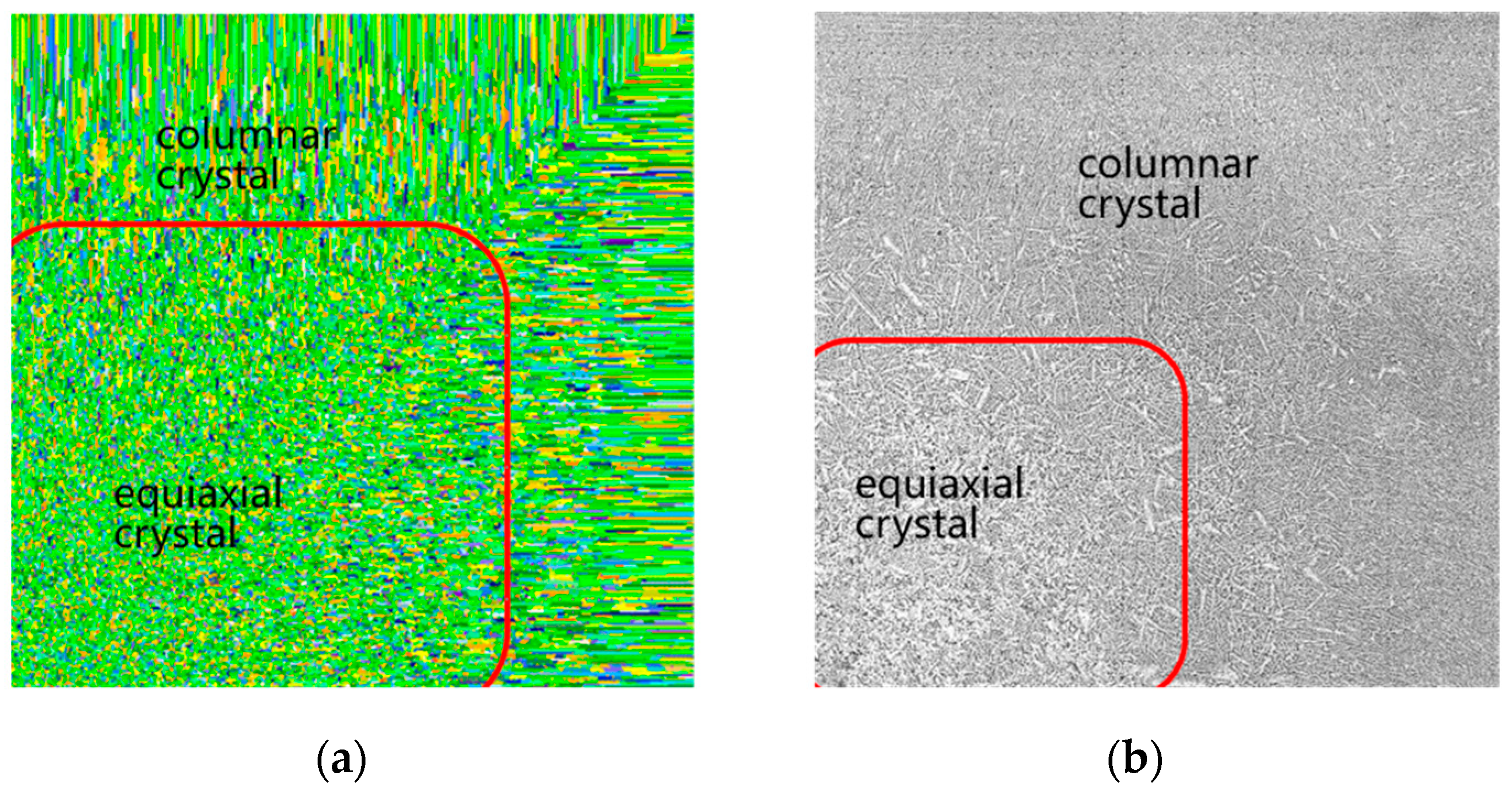
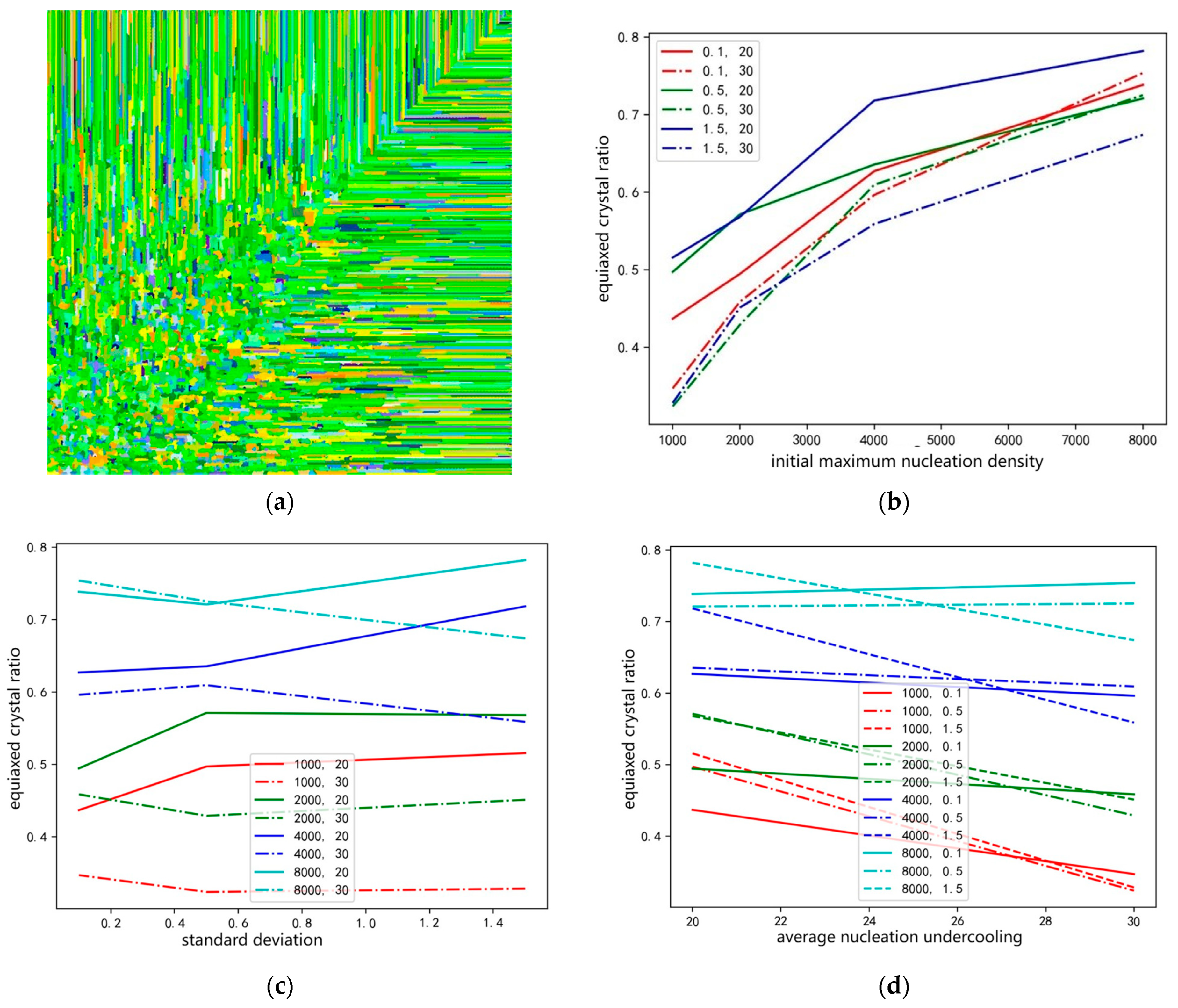
3. Analysing the Effect of Solidification Structure Feature-Recognition Errors on the Fitted Parameters

The recognition error was simulated by adding random Gaussian noise to the equiaxed crystal ratio and length–width ratio data. We added 1000 groups of random noise within 20% error to the equiaxed crystal ratio and length–width ratio data, respectively, and the noise distribution is shown in Figure 4. The average of the mean square error of the fitting results of the 1000 groups of data was calculated, and the variation of the mean square error is shown in Figure 5. It can be seen from Figure 5 that in a Gaussian noise environment, the recognition error effect on the uncertain parameter fitting increases with increasing variance when the recognition error is less than 20%. Both length–width ratio and equiaxed crystal ratio recognition errors increase linearly, and the recognition error of the length–width ratio has a greater effect on fitting uncertain parameters than the recognition error of the equiaxed crystal ratio.

4. Conclusions

An automated method for estimating the uncertain parameters of solidification models is herein proposed. By analysing the relationship between the solidification structure characteristics and the uncertain parameters, we found that the variation of the standard deviation has a small effect on the equiaxed crystal ratio. A model for parameter estimation was established using the estimated uncertain parameters of the solidification model to simulate the low-magnification image, thus obtaining the equiaxed crystal ratio. The maximum error with the real value is 3%, and the minimum error is only 1%. The experiment shows that this method can improve the accuracy of estimating the parameters of the solidification model. By simulating the identification errors of the solidification tissue features, it was found that as the identification errors of the features such as the equiaxed crystal ratio and the dendrite aspect ratio increased, the effect on the fitting parameters increased roughly linearly. This work provides valuable information for estimating solidification model parameters.

References

1. Zhong, H.; Wang, R.; Han, Q.; Fang, M.; Yuan, H.; Song, L.; Xie, X.; Zhai, Q. Solidification structure and central segregation of 6Cr13Mo stainless steel under simulated continuous casting conditions. J. Mater. Res. Technol. 2022, 20, 3408–3419. [Google Scholar] [CrossRef]
2. Zhan, F.; Liu, X.; Zhang, H.; Wang, K.; Xu, S.; Zhu, M.; Zheng, Y.; La, P. Evolution of Structure and Properties of Micro-Nano Structure 2507 Duplex Stainless Steel Prepared by Aluminothermic Reduction. Crystals 2022, 12, 848. [Google Scholar] [CrossRef]
3. Wang, L.; Xing, H.; Li, Y.; Wang, J. Toward multiscale simulations for solidification microstructure and micro segregation for selective laser melting of nickel-based superalloys. J. Mater. Res. Technol. 2023, 25, 3574–3587. [Google Scholar] [CrossRef]
4. Hou, Z.; Jiang, F.; Cheng, G. Solidification Structure and Compactness Degree of Central Equiaxed Grain Zone in Continuous Casting Billet Using Cellular Automaton-Finite Element Method. ISIJ Int. 2012, 52, 1301–1309. [Google Scholar] [CrossRef]
5. Qu, T.; Wang, D.; Wang, H.; Hou, D.; Tian, J.; Hu, S.-Y.; Su, L.-J. Interface characteristics between TiN and matrix and their effect on solidification structure. J. Iron Steel Res. Int. 2021, 28, 1149–1158. [Google Scholar] [CrossRef]
6. Yang, Z. Effect of Electromagnetic Stirring on Molten Steel Flow and Solidification in Bloom Mold. J. Iron Steel Res. Int. 2014, 19, 1766–1776. [Google Scholar] [CrossRef]
7. Priya, P.; Mercer, B.; Huang, S.; Aboukhatwa, M.; Yuan, L.; Chaudhuri, S. Towards prediction of microstructure during laser based additive manufacturing process of Co-Cr-Mo powder beds. Mater. Des. 2020, 196, 109117. [Google Scholar] [CrossRef]
8. Li, J.; Wu, H.T.; Liu, Y.; Sun, Y.-H. Solidification structure simulation and casting process optimization of GCr15 bloom alloy. China Foundry 2022, 19, 63–74. [Google Scholar] [CrossRef]
9. Jia, Y.; Zhao, D.; Li, C.; Bao, L.; Le, Q.; Wang, H.; Wang, X. Study on Solidification Structure Evolution of Direct-Chill Casting High Purity Copper Billet Using Cellular Automaton-Finite Element Method. Metals-Open Access Metall. J. 2020, 10, 1052. [Google Scholar] [CrossRef]
10. Egole, C.P.; Mgbemere, H.E.; Sobamowo, G.M.; Lawal, G.I. Micro-Macro Model for the Transient Heat and Fluid Transport in Solidification Structure Evolution during Static Casting Processes. Mater. Today Commun. 2021, 28, 102613. [Google Scholar] [CrossRef]
11. Jiang, D.; Wang, R.; Zhang, Q.; Zhang, Z.; Wang, B.; Ren, Z. Experimental investigation on solidification of GCr15 bearing steel by the simulated continuous casting. In Ironmaking & Steelmaking; Taylor & Francis: London, UK, 2018; pp. 1–8. [Google Scholar]
12. Karimi, P.; Sadeghi, E.; Ålgårdh, J.; Keshavarzkermani, A.; Esmaeilizadeh, R.; Toyserkani, E.; Andersson, J. Columnar-to-equiaxed grain transition in powder bed fusion via mimicking casting solidification and promoting in situ recrystallization. Addit. Manuf. 2021, 46, 102086. [Google Scholar] [CrossRef]
13. Ouyang, J.H.; Nowotny, S.; Richter, A.; Beyer, E. Characterization of laser clad yttria partially-stabilized ZrO2 ceramic layers on steel 16MnCr5. Surf. Coatings Technol. 2001, 137, 12–20. [Google Scholar] [CrossRef]
14. Guangfeng, Y.; Annan, W.; Chunwei, S.; Jing, C. Numerical simulation and surface morphology of laser cladding of nickel-based C276 alloy coatings on AerMet100 steel surface. J. Mater. Res. Technol. 2023, 27, 1696–1710. [Google Scholar] [CrossRef]
15. Ma, J.; Niu, X.Y.; Zhou, Y.; Li, W.; Liu, Y.; Shen, M.; Wang, H.; Cheng, W.; You, Z. Simulation of solidification microstructure evolution of 316L stainless steel fabricated by selective laser melting using a coupled model of smooth particle hydrodynamics and cellular automata. J. Mater. Res. Technol. 2023, 27, 600–616. [Google Scholar] [CrossRef]
16. Li, X.; Zhang, Z.; Lv, M.; Fang, M.; Liu, K. Numerical Simulation of the Fluid Flow, Heat Transfer, and Solidification in Ultrahigh Speed Continuous Casting Billet Mold. Steel Res. Int. 2022, 93, 2100673. [Google Scholar] [CrossRef]
17. Trindade, L.B.; Nadalon, J.E.A.; Contini, A.C.; Barroso, R.C. Modeling of Solidification in Continuous Casting Round Billet with Mold Electromagnetic Stirring (M-EMS). Steel Res. Int. 2017, 88, 1600319. [Google Scholar] [CrossRef]
18. Wang, J.; Wang, H.; Cheng, X.; Zhang, B.; Wu, Y.; Zhang, S.; Tian, X. Prediction of solidification microstructure of titanium aluminum intermetallic alloy by laser surface remelting. Opt. Laser Technol. 2022, 147, 107606. [Google Scholar] [CrossRef]
19. Travyanov, A.Y.; Petrovskiy, P.V.; Turichin, G.A.; Zemlyakov, E.V.; Kovac, M.; Vondracek, S.; Kondratiev, A.; Khvan, A.V.; Cheverikin, V.V.; Ivanov, D.O.; et al. Prediction of solidification behaviour and microstructure of Ni based alloys obtained by casting and direct additive laser growth. Mater. Sci. Technol. 2015, 32, 746–751. [Google Scholar] [CrossRef]
20. Xue, X.; Xu, L. Numerical Simulation And Prediction Of Solidification Structure And Mechanical Property Of A Superalloy Turbine Blade. Mater. Sci. Eng. A 2009, 499, 69–73. [Google Scholar] [CrossRef]
21. Tonks, M.R.; Aagesen, L.K. The phase field method: Mesoscale simulation aiding material discovery. Annu. Rev. Mater. Res. 2019, 49, 79–102. [Google Scholar] [CrossRef]
22. Zhu, M.F.; Lee, S.Y.; Hong, C.P. Modified cellular automaton model for the simulation of dendritic growth with melt convection. Phys. Rev. E 2004, 69, 061610. [Google Scholar] [CrossRef] [PubMed]
23. Luo, S.; Wang, W.; Zhu, M. Cellular automaton modeling of dendritic growth of Fe-C binary alloy with thermosolutal convection. Int. J. Heat Mass Transf. 2018, 116, 940–950. [Google Scholar] [CrossRef]
24. Natsume, Y.; Oka, Y.; Ogawa, J.; Ohno, M. Estimation of time-dependent heat transfer coefficient in unidirectional casting using a numerical model coupled with solidification analysis and data assimilation. Int. J. Heat Mass Transf. 2020, 150, 119222. [Google Scholar] [CrossRef]
25. Drezet, J.-M.; Rappaz, M.; Grün, G.-U.; Gremaud, M. Determination of thermophysical properties and boundary conditions of direct chill-cast aluminum alloys using inverse methods Metallurg. Mater. Trans. A 2000, 31, 1627–1634. [Google Scholar] [CrossRef]
26. Cheung, N.; Santos, N.S.; Quaresma, J.M.; Dulikravich, G.S.; Garcia, A. Interfacial heat transfer coefficients and solidification of an aluminum alloy in a rotary continuous caster. Int. J. Heat Mass Transf. 2009, 52, 451–459. [Google Scholar] [CrossRef]
27. Gao, W.; Chen, D.; Dai, S.; Wang, X. Back analysis for mechanical parameters ofsurrounding rock for underground roadways based on new neural nework. Eng. Comput. 2017, 34, 25–36. [Google Scholar] [CrossRef]
28. Li, F.-G.; Dong, Q.; Zhang, J.; Dai, Y.-B.; Fu, Y.-N.; Xie, H.-L.; Yin, F.-C.; Sun, B.-D. In situ study on columnar-equiaxed transition and anaxial columnar dendrite growth of Al-15%Cu alloy by synchrotron radiography. Trans. Nonferrous Met. Soc. China 2014, 24, 2112–2116. [Google Scholar] [CrossRef]
29. Liu, P.; Wang, Z.; Xiao, Y.; Mark, F.; Horstemeyer Cui, X.; Chen, L. Insight into the mechanisms of columnar to equiaxed grain transition during metallic additive manufacturing-ScienceDirec. Addit. Manuf. 2019, 26, 22–29. [Google Scholar]
30. Wang, J.; Meng, H.; Yang, J.; Xie, Z. A fast method based on GPU for solidification structure simulation of continuous casting billets. J. Comput. Sci. 2021, 48, 101265. [Google Scholar] [CrossRef]
31. Thevoz, P.; Desbiolles, J.L.; Rappaz, M. Modeling of equiaxed microstructure formation incasting. J. Metall. Trans. A. 1989, 20, 311–322. [Google Scholar] [CrossRef]
32. Zhu, M.; Hong, C. A modified cellular automaton model for the simulation of dendritic growth in solidification of alloys. ISIJ Int. 2007, 41, 436–445. [Google Scholar] [CrossRef]
33. Jing, C.L.; Wang, X.H.; Jiang, M. Study on Solidification Structure of Wheel Steel RoundBillet Using FE-CA Coupling Model. Steel Res. Int. 2011, 82, 1173–1179. [Google Scholar] [CrossRef]
34. Invanstov, G.P. Temperature field around spherical, cylindrical, and needle-shapedcrystals which grow in supercooled melts J1. Dokl. Akad. Nauk. SSSR 1947, 58, 567–570. [Google Scholar]
35. Yamazaki, M.; Natsume, Y.; Harada, H. OhStructure Formation during Continuousasting in Fe-0.7mass%C Alloy Using Cellular Automaton Method. ISIJ Int. 2006, 46, 903–908. [Google Scholar] [CrossRef]
Figure 1. (a) Simulation image; (b) actual low-magnification image.
Crystals 13 01673 g001
Figure 2. (a) Numerical simulation image. (b) Relationship between initial maximum nucleation density and equiaxed crystal ratio. (c) The relationship between average nucleation undercooling and equiaxed crystal ratio. (d) Relationship between standard deviation and equiaxed crystal ratio.
Crystals 13 01673 g002
Figure 3. (a) Simulated image with standard deviation of 0.1. (b) Simulated image with standard deviation of 1.5. (c) Difference images of (a) and (b).
Crystals 13 01673 g003
Figure 4. (a) Error distribution for equiaxed crystal ratio of 0.56 error. (b) Error distribution for equiaxed crystal ratio of 0.63. (c) Error distribution for length–width ratio of 99. (d) Error distribution for length–width ratio of 125.
Crystals 13 01673 g004
Figure 5. Variation diagram of equiaxed crystal ratio and dendrite length–width ratio error.
Crystals 13 01673 g005