Article

Determination of Heat Transfer Coefficient by Inverse Analyzing for Selective Laser Melting (SLM) of AlSi10Mg

1
College of Mechanical Engineering, Donghua University, Shanghai 201620, China
2
Shanghai Academy of Space Flight Technology, Shanghai 201109, China
3
School of Mechanical Engineering, University of Shanghai for Science and Technology, Shanghai 200093, China
4
Aplos Machines Manufacturing (Shang Hai) Co., Ltd., Shanghai 201306, China
*
Author to whom correspondence should be addressed.
Crystals 2022, 12(9), 1309; https://doi.org/10.3390/cryst12091309
Submission received: 1 September 2022 / Revised: 1 September 2022 / Accepted: 9 September 2022 / Published: 16 September 2022
(This article belongs to the Special Issue Processing Technology of Brittle Crystal Materials)

Abstract

:
Heat treatment can improve performance and control quality in the additive manufacturing process. In the numerical simulation of heat treatment, the accuracy of the heat transfer coefficient will have a significant impact on the accuracy of the simulated temperature field. At present, The inverse analysis method is the most common and effective method to determine the heat transfer coefficient. Taking the actual temperature curve as the input condition, the heat transfer coefficient values of the heating, quenching, and air cooling components in the heat treatment process are successfully obtained. Based on the obtained heat transfer coefficient, a mathematical model of the heat transfer coefficient change with temperature during heat treatment is established. The heat transfer coefficient obtained by the inverse analysis method is then applied to the simulation of heat treatment, and more accurate simulation results are obtained. It is proven in this work that the inverse analysis method can improve the accuracy of the simulation model in the heat treatment process of AlSi10Mg.

1. Introduction

For the manufacturing process of parts, the traditional material removal [1,2,3] has been extended to printing parts through additive manufacturing. The combination of additive and subtractive processing technology helps to produce more multifunctional complex structures [4,5,6]. The aluminum alloy AlSi10Mg is a typical alloy with significantly improved strength and hardness, which is suitable for thin-walled, complex geometrical parts in automotive, aerospace and aerospace industrial-grade prototypes and production components [7,8]. AlSi10Mg is widely used in additive manufacturing. The effect of heat treatment on improving additive manufacturing process can be analyzed by heat treatment of parts made of this material.
There are many factors affecting the heat transfer coefficient [9,10,11], and it is difficult to accurately solve the interfacial heat transfer coefficient by using the conventional surface temperature and temperature gradient methods. The inverse analysis method is the most common and effective method to solve the heat transfer coefficient. First of all, temperature data [12,13,14] in the heat treatment process were obtained through experimental measurement, and the data were imported into DEFORM. The optimal program in DEFORM compared simulated time and temperature data with experimental time and temperature data, and optimized the operation until the optimal value was calculated.
Shokoufeh et al. [15] used CFD simulation to explore the heat transfer during the heat up portion of the curing cycle in an autoclave to improve the production rate without compromising quality. Su et al. [16] investigated the heat transfer performance of electrostatic spraying used in machining using the newly developed device by transient heat transfer tests. Kim et al. [17] calculated the interfacial heat transfer coefficient between the die and the workpiece, using the inverse analysis method to measure the temperature of the die in the hot stamping process. Gianfranco et al. [18] took the temperature data of the process collected by thermocouple as the input value, and simulated the whole sand mold casting process with the commercial software package MAGMASOFT using the finite difference method. By increasing the number of temperature control points, the interfacial heat transfer coefficient was obtained. Using the temperature data of sand and metal collected by thermocouple, Sun Mikhail et al. [19] presented a technique for process-induced residual strain modeling for thermoset composite material parts and used the technique to clarify the distribution of the heat transfer coefficient on the surface of the part and mold using the CFD method. And distribution of heat transfer coefficients were obtained in ANSYS CFX under the appropriate process conditions. Modeling simplifications were proposed by Ramos et al. [20] for an efficient numerical discretization of infill structures. With the prospect of choosing correct thermal boundary conditions expressing the natural convection between printed material and its environment, values for the convective heat transfer coefficient and ambient temperature were calibrated through numerical data fitting of experimental thermal measurements. Kadam et al. [21] proposed an inverse method based on the transient temperature of the back surface using the solution of the three-dimensional inverse heat conduction problem to estimate the transient temperature of the collision side and then evaluate the heat transfer coefficient. Kang et al. [22] proposed an empirical formula for laminar natural convection of an outer finned tube heat exchanger with a wide range of structural parameters and calculated the heat transfer coefficient by using the transient temperature response of the heat exchanger. Piotr [23] simplified the three-dimensional transient heat conduction problem to an axisymmetric heat conduction problem and used the inverse method to calculate the surface heat transfer coefficient. Farzad et al. [24] used three-dimensional elliptic mesh generation technology to mesh irregular bodies. A new and highly effective sensitivity analysis program was introduced to the gradient-based optimization method to calculate the sensitivity coefficient, and a more accurate thermal conductivity, heat transfer coefficient, and heat flux density could be obtained by this solution.
With the development of intelligent algorithms, some new inverse analysis methods have emerged in recent years. Parida et al. [25] used Green’s function method considering transient convective boundary conditions and transient radiant heat loss to estimate the total heat transfer coefficient and adiabatic heat transfer during the jet impact heat transfer process by inputting the transient temperature of the non-collision surface obtained by the experiment. Zhang et al. [26] introduced the complex variable differentiation method (CVDM) in the commercial finite element software Abaqus, developed a complex variable finite element model by using the user element subroutine (UEL), and accurately calculated the Levenberg-Marquardt algorithm to solve the key parameter sensitivity matrix coefficient of the inverse problem. This technique provided a general method for solving the inverse problem of three-dimensional transient nonlinear heat conduction in irregular and complex structures. Ming et al. [27] established a three-way equivalent heat conduction model including heat conduction and heat convection in the cutting process based on the structural characteristics of the honey comb core. After using the inverse calculation process of the Fourier number characterization model to improve the stability and accuracy of the inverse calculation, the model was used to study the influence of alloy materials and process parameters on the heat transfer coefficient of the casting-mold interface during the die casting process. The functional relationship between the casting-mold interface heat transfer coefficient and the solidification fraction and solidification rate of the die-casting process was also established. At the same time, it was found that, among the die-casting process parameters, the initial surface temperature of the mold had the greatest influence on the heat transfer coefficient [28,29,30]. Chen et al. [31] proposed to take the screw as a one-dimensional rod heat transfer system to solve the thermal error of the screw by establishing a thermal characteristic equation. In Ho et al.’s [32] investigation, two commercial-scale porous lattice heat exchangers of different lattice unit cell sizes were fabricated by SLM. Experiments were performed in a wind tunnel to characterize the thermal-hydraulic performances of the heat exchangers. Jiang et al. [33] explored the effects of heat treatment on microstructure and residual stress of SLM AlSi10Mg alloy. Wang et al. [34] reported a study of condensation heat transfer and pressure drop of R-134a inside four enhanced tubes and one plain tube fabricated by SLM. The effects of fin height, refrigerant flow direction and mass flux on the heat transfer coefficient and pressure drop were studied. Martin et al. [35] presented an experimental study of the mechanical strength and numerical analysis of the thermal behaviour during SLM fabrication of ALSi10Mg block support structures.
In Huiping et al.’s [36] investigation, A new method to calculate the temperature-dependent surface heat transfer coefficient during quenching process is presented, which applies finite-element method (FEM), advance–retreat method and golden section method to the inverse heat conduction problem, and can calculate the surface heat transfer coefficient according to the temperature curve gained by experiment. In Apmann et al.’s [37] research, the influence of the connector between the two microchannels was studied. By studying the effect of Reynolds number and the introduction of nanoparticles into the base liquid on the heat transfer coefficient of the connector, it was shown that these two factors played an important role in the influence of the connector on the heat transfer coefficient. Khooshehchin et al. [38] studied the effects of vertical and horizontal surface roughness on bubble dynamics and heat transfer coefficient during pool boiling. The experimental results showed that with the increase of surface roughness, the nucleation position increases, leading to the enhancement of heat transfer. The experimental data were verified by a conventional model. This paper aims to import the temperature data measured in the experiment into DEFORM and calculate the heat transfer coefficient in the heat treatment process through its inverse heat conduction module. As professional finite element software for volume forming, DEFORM-3D can not only simulate the thermodynamic coupling calculation of the workpiece heat treatment process, but also directly solve the heat transfer coefficient between the workpiece and the medium with its inherent Inverse Heat Transfer Wizard model [39]. Using the DEFORM Inverse Heat Transfer model to solve the surface heat transfer coefficient involves the selection and determination of parameters such as temperature control point and the initial value of the surface heat transfer coefficient. The reasonable selection of these parameters will have a significant influence on the calculated value of the surface heat transfer coefficient and the predicted temperature field [40]. In this paper, the temperature curve in the heating and cooling process in the heat treatment process is obtained through experiments, and the finite element model is established to solve the heat transfer coefficient [41]. By adjusting the initial value of the heat transfer coefficient, the simulated temperature curve corresponds closely to the experimental results to obtain an accurate heat transfer coefficient value, and the heat transfer coefficient results obtained by the solution are fitted to establish the mathematical relationship between the heat transfer coefficient and the temperature.

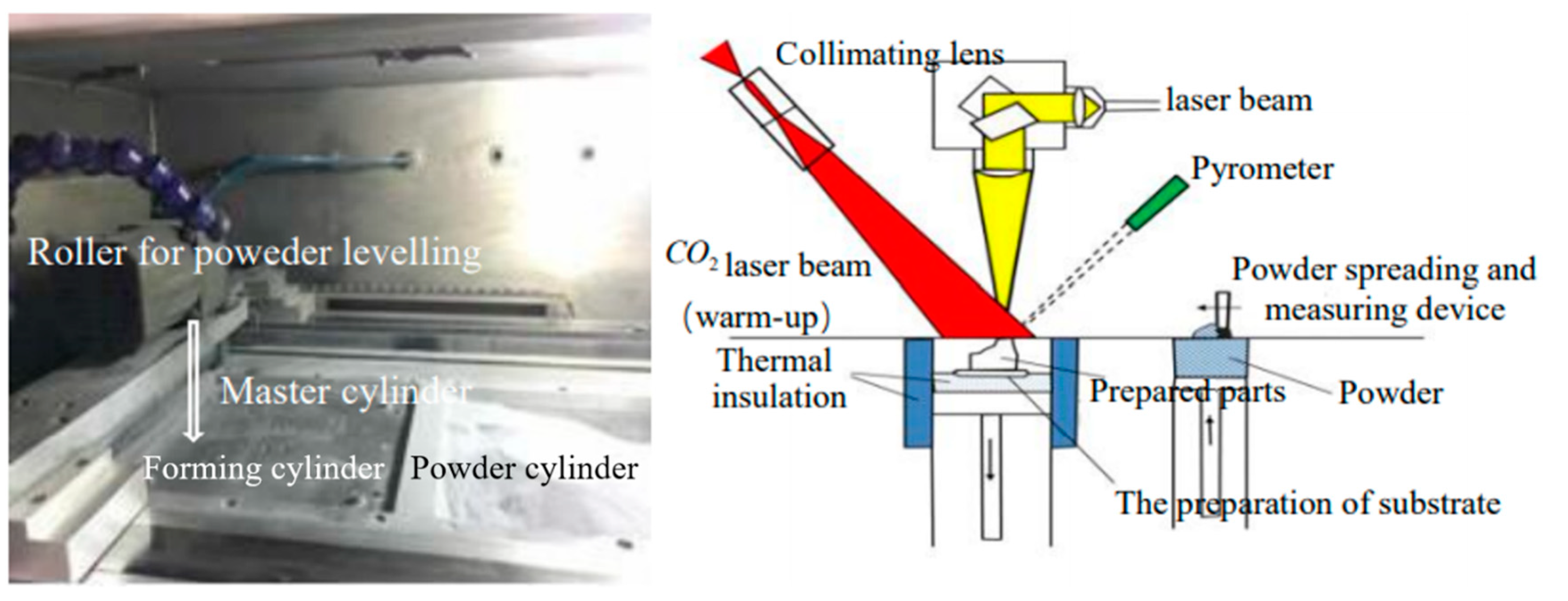
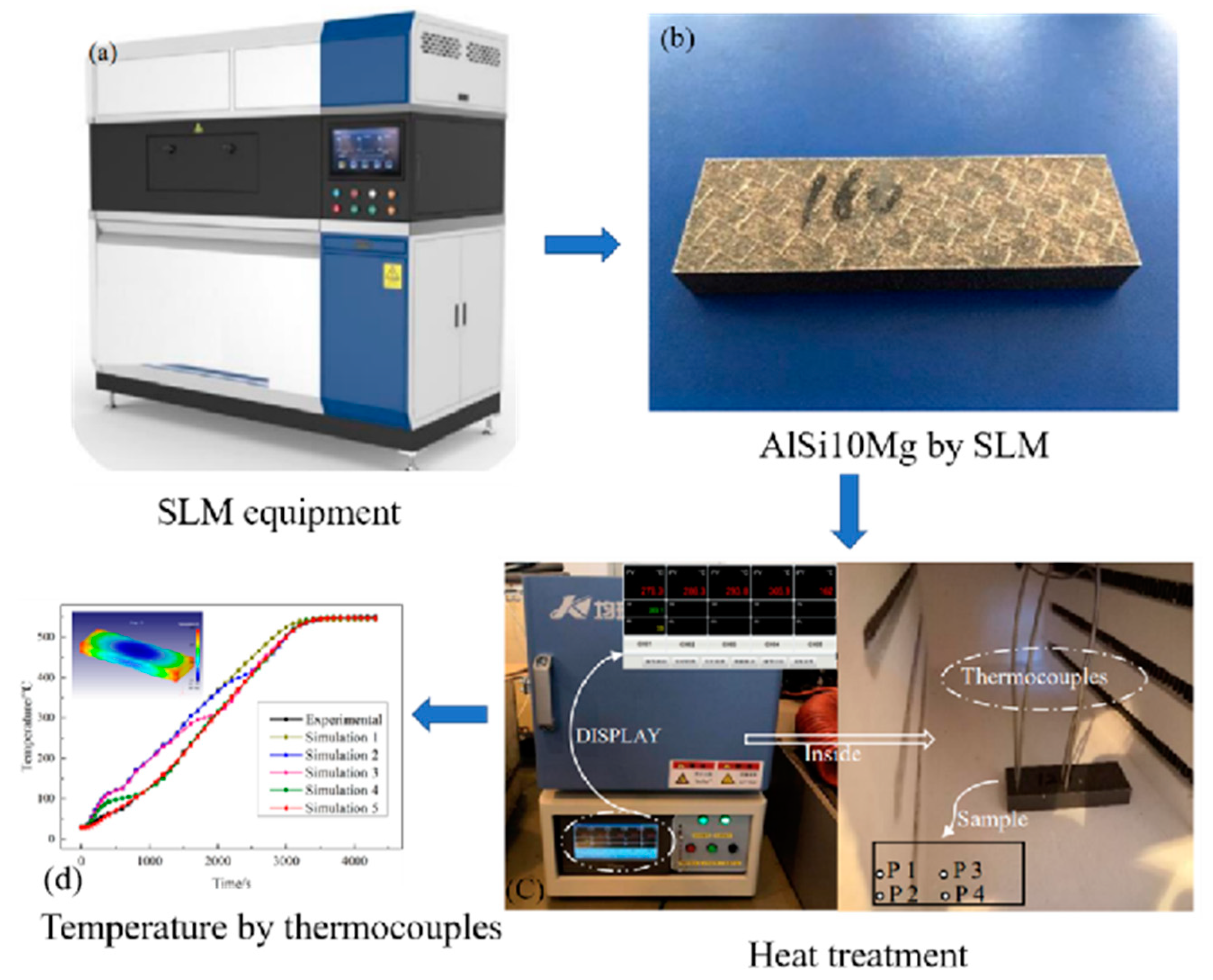
2. Experimental Procedure

The AlSi10Mg alloy molded by selective laser melting (SLM) used in this experiment was manufactured by the Space M200 manufacturing system (Figure 1). In the SLM process, the thermocouples are installed on the substrate for measurement, that is, “The preparation of substrate” shown in Figure 1. This research uses thermocouples to measure temperature data during subsequent heat treatment of molded samples. The print size was 250 mm × 250 mm × 250 mm, and the sample size was 40 mm × 30 mm ×80 mm. The SLM molding process parameters used in this project were laser power of P = 400 W, laser scanning speed of v = 200 mm/s, a scanning layer thickness of 50 μm, scanning time interval of 150 μm, and a preheating temperature of 80 °C.
A JXR1200-30 muffle furnace was used in the heat treatment process.
As shown in Figure 2a, shows the SLM printing equipment.The working size was 300 mm × 150 mm × 150 mm, the highest operating temperature was 1200 °C, and a high quality resistance wire containing molybdenum was used as the heating element. The Proportional Integral Derivative (PID) control mode and a K type thermocouple were employed, and the constant temperature accuracy was ±1 °C. In this experiment, the size of the AlSi10Mg sample was 8 mm × 25 mm × 80 mm(Figure 2b). When the measurement depth of the thermocouple is 4 mm, it can measure the temperature data in the center area of the sample. In order to ensure that the results of different regions are representative, four points are selected in different locations for analysis, which can be used for comparison and verification of simulation results. Therefore, four holes were punched in the workpiece to a depth of 4 mm, and a thermocouple was installed to measure the real-time temperature (Figure 2c). As shown in Figure 2c, the thermocouple is inserted into a small hole on the surface of the sample to measure and obtain the temperature data during the heat treatment process in real time. In order to reduce the experimental error and ensure the reliability of the temperature data, three groups of the same temperature measurement experiments were done, and the temperature data were not different. The average temperature was imported into DEFORM as an input parameter to solve the heat transfer coefficient of each stage. As shown in Figure 2d, shows the comparison curve of the measured temperature and the simulated temperature.
As shown in Figure 2, based on the above experimental conditions, time-temperature data of each stage in the heat treatment process can be measured, which will be used as input parameter when solving the heat transfer coefficient of each stage with DEFORM.

3. Modeling Procedure

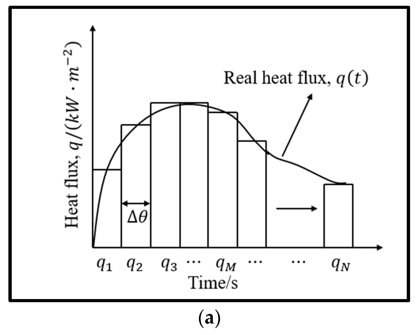
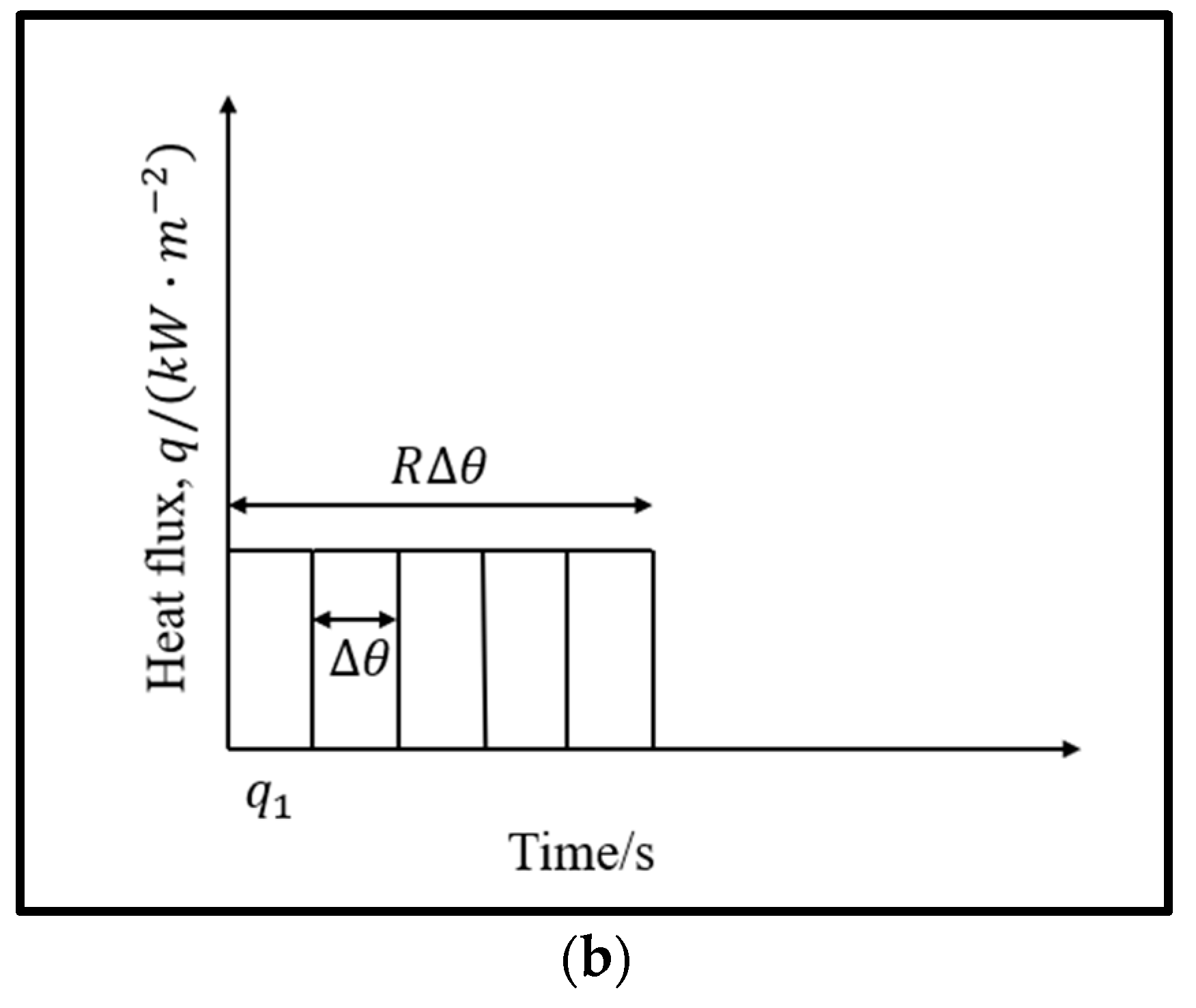
3.1. Mathematical Model

In the process of heat treatment, heat conduction is the main mechanism inside the workpiece. The three-dimensional heat conduction differential equation is:
ρ c T t = x λ T x + y λ T y + z λ T z + Q ˙
where ρ is density, kg / m 3 ; c is the specific heat capacity, J/(kg °C); T is temperature, °C; t is time, s ; Q ˙ is the heat generated by the internal heat source, W / m 3 ; λ is the thermal conductivity coefficient, W/(m °C).
Initial conditions are the starting point of calculation. To solve the above equation, initial conditions must be given. Quenching starts from room temperature furnace heating, at this time:
T x = 0 = T 0
where T 0 is the known temperature and is a constant.
The boundary conditions of heat transfer generally fall into the following three categories:
(1) When the boundary function is known, it is the first kind of the boundary condition:
T s = T w x , y , z , t
where, s is the boundary range, x , y , z are coordinate values, and t is time.
(2) When the surface heat flux q w of the object is known, it is the second kind of the boundary condition:
k T n s = q w z , r , t
where, q w is the heat flux of the workpiece surface.
(3) The third kind of boundary condition, also known as Newton boundary conditions, are given for the convective heat transfer coefficient on the boundary surface:
k T n s = h k T w T f
where, h k is the heat transfer coefficient, T w is the workpiece temperature, and T f is the medium temperature.
Inverse heat transfer Wizard in DEFORM was used to solve the inverse heat conduction problem, and the algorithm was based on Beck’s regularization law. In the solution process, the heat conduction inverse algorithm is determined according to the nonlinear estimation method of Beck et al. [40,41], as shown in Figure 3a,b. The heat flux varying with time can be discretized into a number of heat flux values with time intervals of Δ θ q i = q 1 , q 2 q M q N . In order to improve the stability of the inverse algorithm, the concept of future time step is introduced when solving the heat flow at a certain moment; that is, the heat flow values within the following time interval are assumed to be equal. Thus:
q M = q M + 1 = q M + 2 = = q M + R
Each heat flow is obtained through the iterative calculation of the criterion of the minimum error value of temperature measurement and calculation, which can be expressed by the following formula:
F q M = i = 1 N   j = 0 r 1 T i ,   M + j m T i , M + j c 2
where T i ,   M + j m is the actual measured temperature at the measuring point i in the time period of M + j ;   T i , M + j c is the temperature calculated and solved at the measuring point i in the time period of M + j ;   N is the total number of temperature points measured; r is the total number of the future period of the measurement point.
Minimization is the main objective in the following calculation. To solve the extreme value of F q M , the derivative of the above expression is taken and set as equal to 0, obtaining:
i = 1 N   j = 0 r 1 T i ,   M + j m T i , M + j c   T i , M + j c q M = 0
In order to solve T i , M + j c and T i , M + j c q M , Taylor series expansion is applied to T i , M + j c at q M = q M * :
T i , M + j c q M = T i , M + j c q M * + T i , M + j c q M q M q M *
Among them, there are: Δ q M = q M q M * , so:
T i , M + j c q M = T i , M + j c q M * + T i , M + j c q M Δ q M
The equations can be obtained simultaneously as:
Δ q M = i = 1 N   j = 0 r 1 T i ,     M + j m T i , M + j c   T i , M + j c q M i = 1 N   j = 0 r 1 T i , M + j c q M 2
where q M and Δ q M are the interface heat flow value and interface heat flow modification value in the current calculation period, respectively.
Function F is an object function that is computed iteratively. With mathematical derivation, the interface heat flow can be solved by the following two expressions:
Δ q M = j = 1 J   i = 1 R T j , M + i C j , M + i ϕ j , M + i j = 1 J   i = 1 R ϕ j , M + i 2
q M + 1 = q M + Δ q M
where ϕ j , M + i is the sensitivity coefficient, which is defined as the response of temperature at a certain position in the casting or mold with the change of unit heat flow, and is expressed as:
ϕ j , M + i = T j , M + i q j , M + i
In the iterative calculation of heat flow, q M is modified continuously with the above formula. When the difference between the measured temperature and the calculated temperature meets the given convergence error, the currently calculated heat flow q M can be obtained. The process is repeated until the heat flow q at all times is calculated.
When the heat flow q at all times is solved, the surface heat transfer coefficient can be obtained by the following equation:
H = q / T w T c
where H is the surface heat transfer coefficient/N/(mm s °C); T w is the workpiece surface temperature/°C; T c is the medium temperature/°C.
The DEFORM reverse heat transfer model first assumes the initial value of the surface heat transfer coefficient and calculates the internal temperature value through the thermal conductivity differential equation. It then continuously revises the set value according to the difference between the calculated value and the experimentally measured value and, finally, makes the calculated value approach the measured value. The accuracy of the calculated surface heat transfer coefficient can be determined by comparing the predicted temperature value with the measured one.

3.2. Finite Element Model

An AlSi10Mg alloy sample printed by selective laser melting (SLM) is investigated in this work. A rectangular parallelepiped sample with a length of 80 mm, width of 25 mm, and height of 8 mm is selected. This alloy has the advantages of high strength, good thermal performance, and light weight. AlSi10Mg powder is spherical; its chemical composition is shown in Table 1 and is within the size of 20~63 um, prepared by the atomization method.
Due to the vigorous development of metal 3D printing technology in recent years, the sample of AlSi10Mg alloy formed by SLM is a relatively new material. Thus no corresponding material is available in the material libraries of the simulation software, and we must establish a new material model here.
In the process of material transformation changing with temperature, the thermophysical parameters change non-linearly. Table 2 and Table 3 shows the thermophysical parameters and the mechanical property parameters of AlSi10Mg. Physical parameters of materials are crucial to the prediction accuracy of the model. The physical parameters of AlSi10Mg alloy referenced by the model in this subject are as follows.

4. Results and Discussion

The inverse problem of heat conduction is a relatively important inverse problem. It has important guiding significance to improve the accuracy of simulation model, determine and predict the temperature field, and further improve the efficiency of heat treatment. In this paper, through constructing the simulation model of the AlSi10Mg alloy sample, the inverse calculation of heat conduction is carried out in the Inverse Heat Transfer Wizard module of DEFORM. As shown in Figure 4, the specific operation is to heat-treat a workpiece, and a thermocouple is used to collect the time-temperature data corresponding to the workpiece during the heat treatment process. The parameters of the simulation part are shown in Table 4. On the one hand, the future time steps will affect the accuracy of the calculation result, on the other hand, it will affect the convergence of the result, that is, it will affect the calculation time.
It is assumed that the initial heat transfer coefficient is constant 1, the initial temperature of the workpiece is 20°, and the temperature distribution is uniform. The simulated ambient temperature is set as the highest temperature obtained during the experiment. Based on the initial assumption of the heat transfer coefficient, the heat transfer coefficient under different temperature conditions is solved. Finally, the simulated time and temperature data are compared with the experimental time and temperature data, and the solution value is input as the initial value for the optimization operation until the optimal value is calculated.
The stages of heat treatment are shown in Figure 5. In the heat treatment process, assuming that the bottom surface of the sample is fully constrained, the inverse calculation of the heat transfer coefficient value of the AlSi10Mg alloy sample can be roughly divided into the following three cases. The first one is the heat transfer coefficient value of the AlSi10Mg alloy during the heating process. The second is the heat transfer coefficient during quenching. The third is the value of the heat transfer coefficient in the process of air cooling.

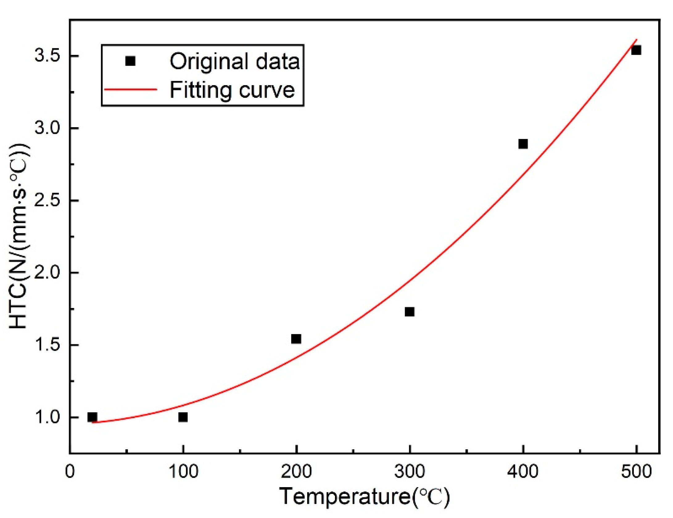
4.1. Detection and Analysis of Heat Transfer Coefficient during Heating

During the heating process, the temperature of the AlSi10Mg alloy sample rises with the temperature in the furnace, and the temperature values at all points change in a relatively consistent way. The temperature data of one point is imported into the Inverse Heat Transfer Wizard module of DEFORM for simulation, and the simulation results are shown in Figure 6.
Figure 7 below shows the simulation results of five inverse calculations. It can be seen from the figure that although the simulated temperature value obtained from the first simulation result differs greatly from the experimental value, the temperature variation trend is completely consistent, indicating that the heat conduction inverse calculation module of DEFORM has reliability. In the second and third simulations, the simulation temperature of the high temperature part is relatively close to the experimental value, but there is still a big difference at low temperature.
The closer the initial value of heat transfer coefficient is to the actual situation, the shorter the calculation time and the more accurate the simulation result is. First of all, set the heat transfer coefficient of the initial value is 1, solving the heat transfer coefficient to get a new set of values, to solve the resulting value used in the simulation of the heat treatment process, comparing the simulation results and experimental results, and then use this value as the initial value to solve the next set of heat transfer coefficient, and used to simulate the heat treatment process, until the simulation results was coincident with the experimental results. By adjusting the heat transfer coefficient at low temperature, after several adjustments of the simulation, the simulation temperature curve gradually fits with the experimental value, the final curve is almost exactly the same, and the fitting effect is good.
Table 5 shows the value of the heat transfer coefficient obtained by the simulation solution. The T here refers to the temperature of the point measured by the thermocouple. The fitting results in Origin are as shown in Figure 8. The following equation is the mathematical model obtained by fitting:
H = 0.95 + 2.97 × 10 4 T + 1 × 10 5 T 2
where H is the value of the heat transfer coefficient, and the unit is N/mm·s·°C × 10−2; T is the temperature, and the unit is °C; R 2 is 0.96.

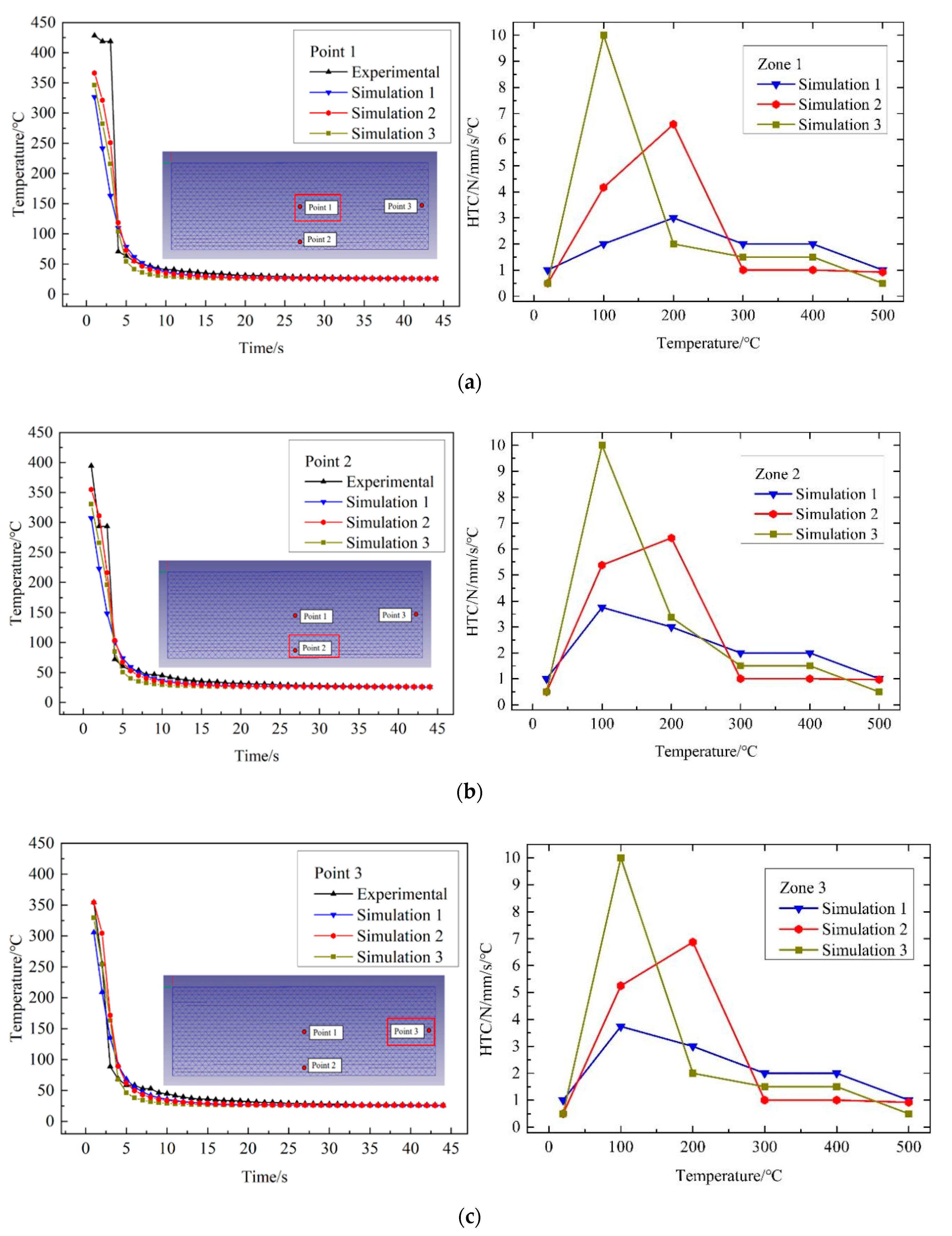
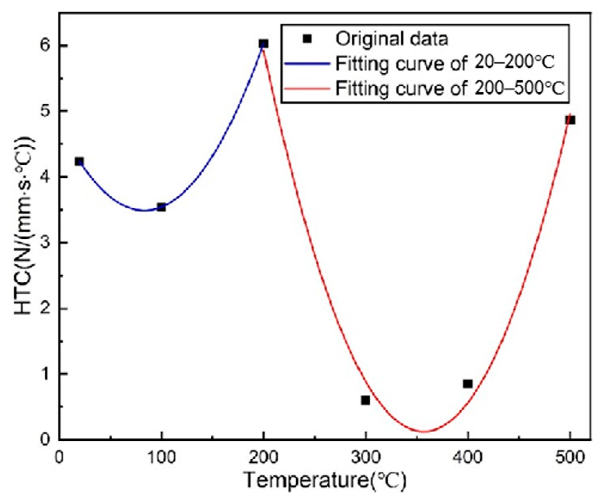
4.2. Detection and Analysis of Heat Transfer Coefficient during Quenching

Due to the good thermal conductivity of aluminum alloy, the cooling rate is large, and the temperature drops quickly during quenching. The temperature drops at each point of the sample are not consistent, and the surface and boundary drop the fastest.
Three points of symmetry on the surface of AlSi10Mg alloy are taken with the depth of 2 mm: point 1 (12.5, 40, 6), point 2 (23, 40, 6) and point 3 (12.5, 77, 6).
As shown in Figure 9, the black upper triangle symbol is the experimental test temperature. During quenching, the temperature drops sharply. Due to the sharp drop in temperature during quenching, the temperature data measured have a sharp decline trend. Among them, in the beginning, the temperature of points 2 and 3 drops with the center point 1. After 3–4 s, the temperature decreases slowly and gradually lowers to room temperature over time.
The selected temperature range ranges from room temperature to the highest temperature used in the heat treatment process. The trend of the simulated temperature data curve is basically the same as that of the experimental temperature data curve, so it can be concluded that the data is selected under the condition that the experimental error allows. Temperature changes at three points in the simulation over time are shown in Figure 9. The decreasing trend of each point is basically consistent with the measured value in the experiment. Compared with the first and third simulations, the simulation value of the second simulation is closer to the experimental value. The results of the three simulations are consistent with the experimental values. However, due to the rapid temperature decline during quenching, the number of measured temperature values is small. As a result, the simulation accuracy is slightly lower than that in the heating process.
Table 6 shows the value of the heat transfer coefficient obtained by the simulation solution. The fitting results in Origin are as shown in Figure 10. The following equation is the mathematical model obtained by fitting:
When the temperature is 20–200 °C:
H = 0.95 + 2.97 × 10 4 T + 1 × 10 5 T 2
When the temperature is 200–500 °C:
H = 0.95 + 2.97 × 10 4 T + 1 × 10 5 T 2
where H is the value of heat transfer coefficient, the unit is N/mm·s·°C × 10−2; T is the temperature, the unit is °C; R 2 is 1 and 0.98, respectively.

4.3. Detection and Analysis of Heat Transfer Coefficient in Air Cooling Process

The indoor temperature is 26 °C during air cooling. The temperature of the surface and edge of the AlSi10Mg alloy sample drops rapidly, but the difference is not significant. The temperature at the center of the sample is taken as the experimental value, and the simulated temperature is obtained by inserting the Inverse Heat Transfer Wizard module, as shown in Figure 11. In the process of temperature drop, the simulation temperature is lower than the experimental value between 42 and 30 °C, while the simulation temperature is slightly higher than the experimental value between 30 °C and room temperature, but the difference is not more than 5 °C.
In the process of air cooling, the temperature basically remains unchanged, that is, the ambient temperature of the sample remains unchanged. The simulated values of heat transfer coefficients in each region are shown in Table 7. The simulated heat transfer coefficient values during air cooling are shown in Table 8.

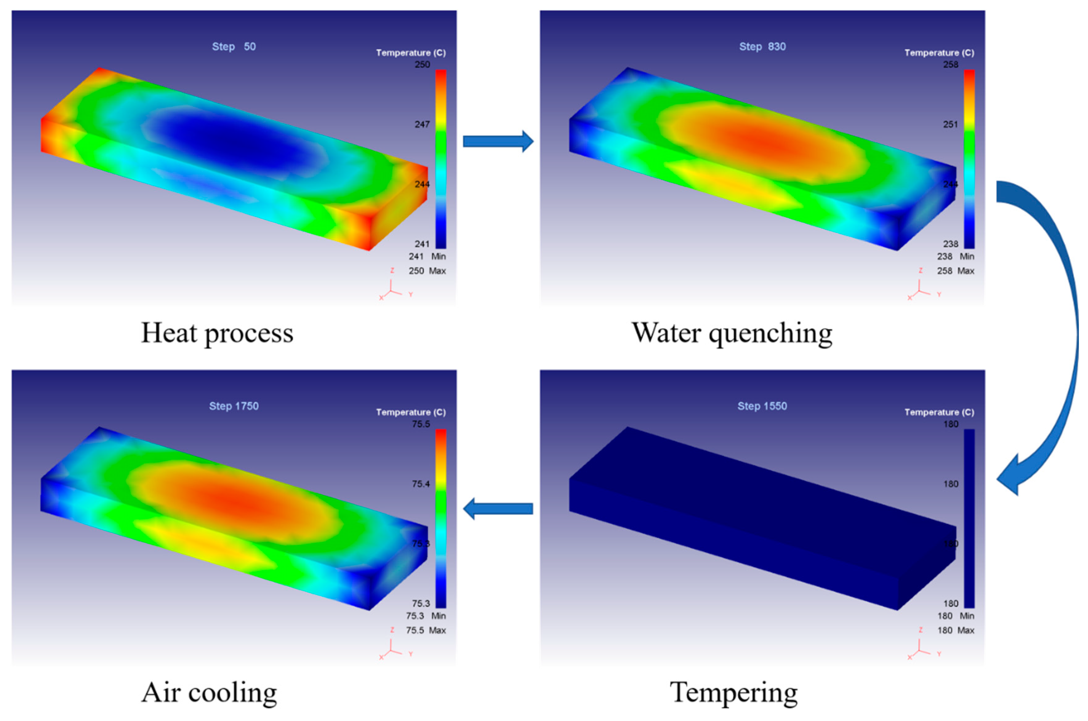
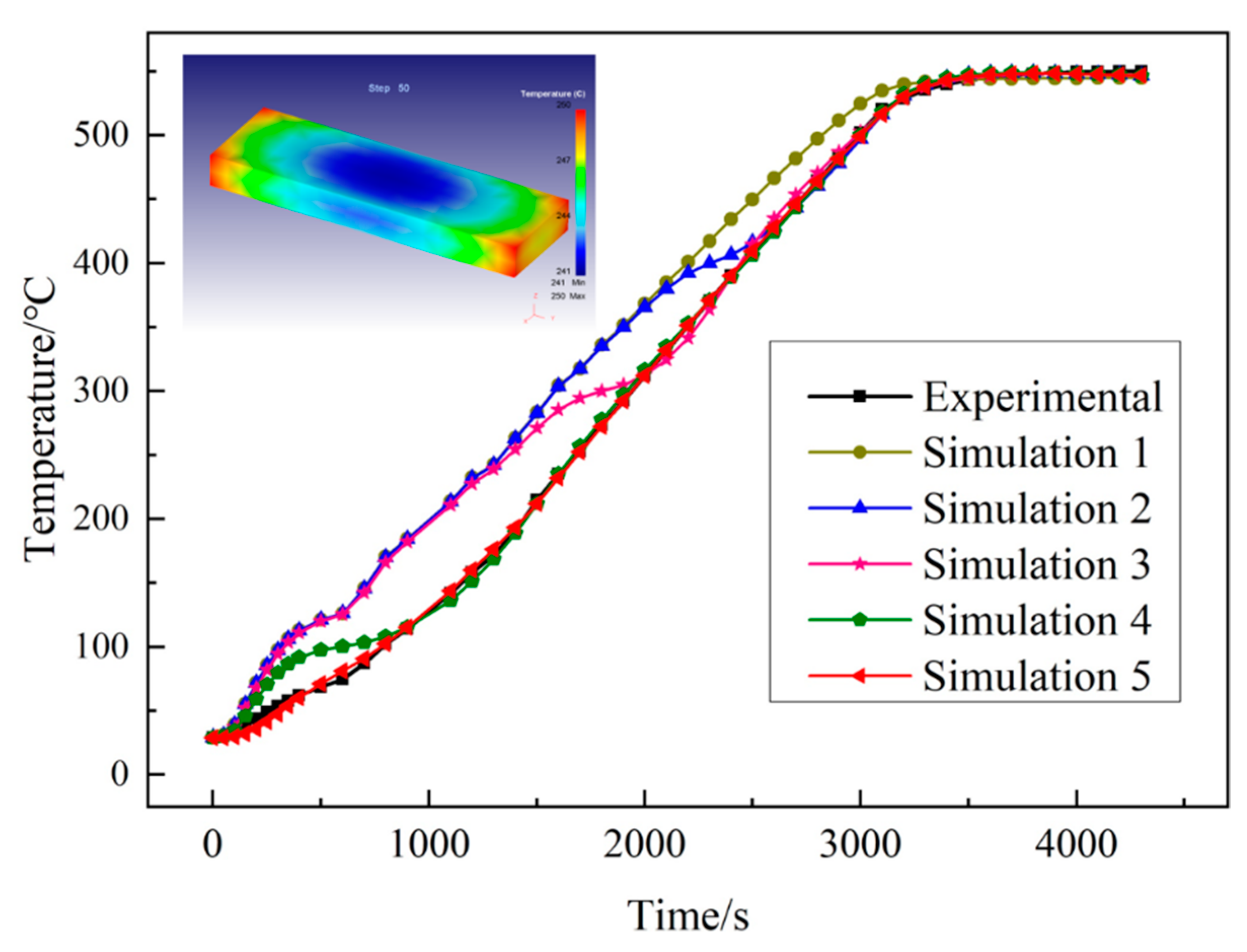
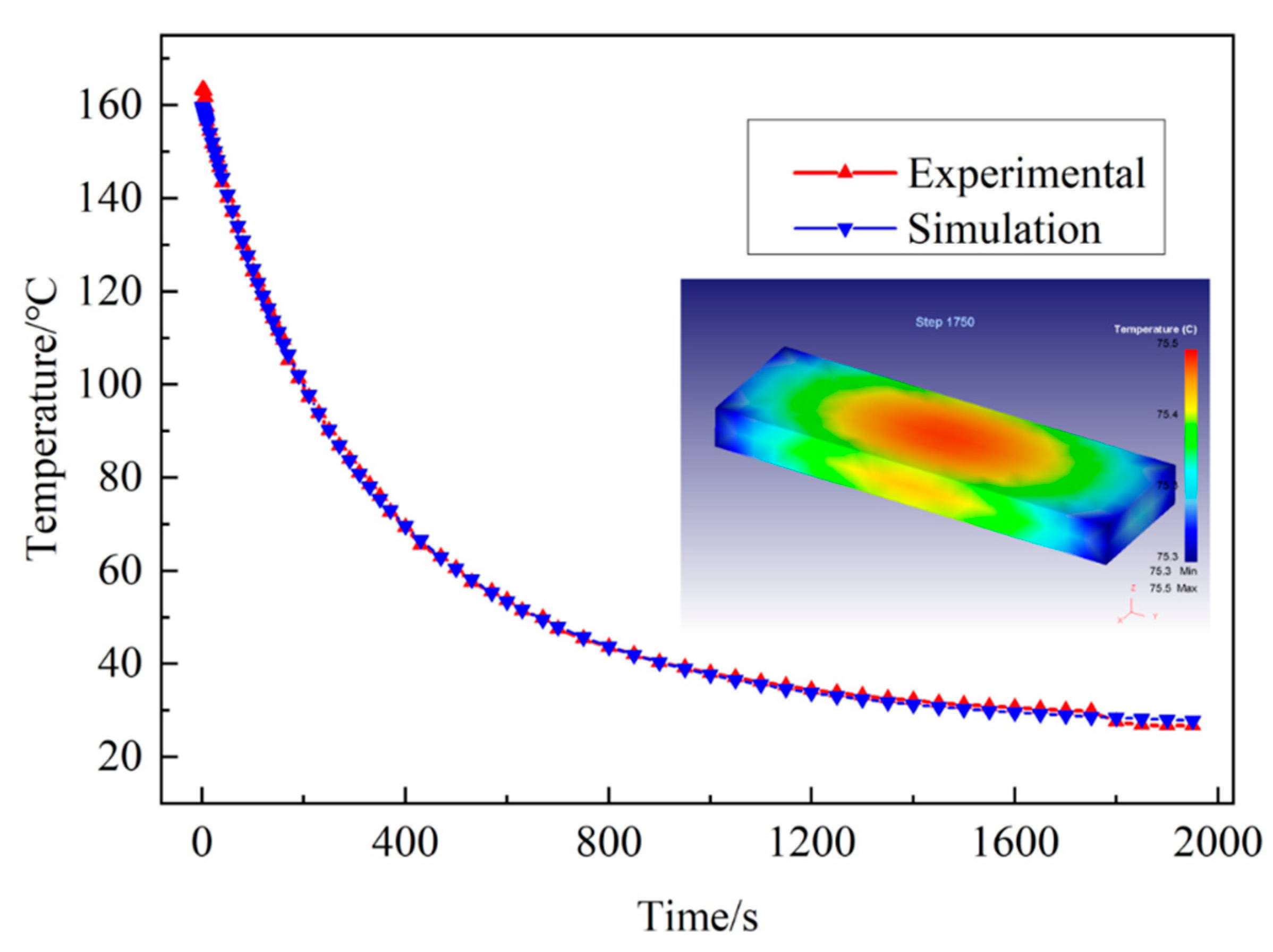
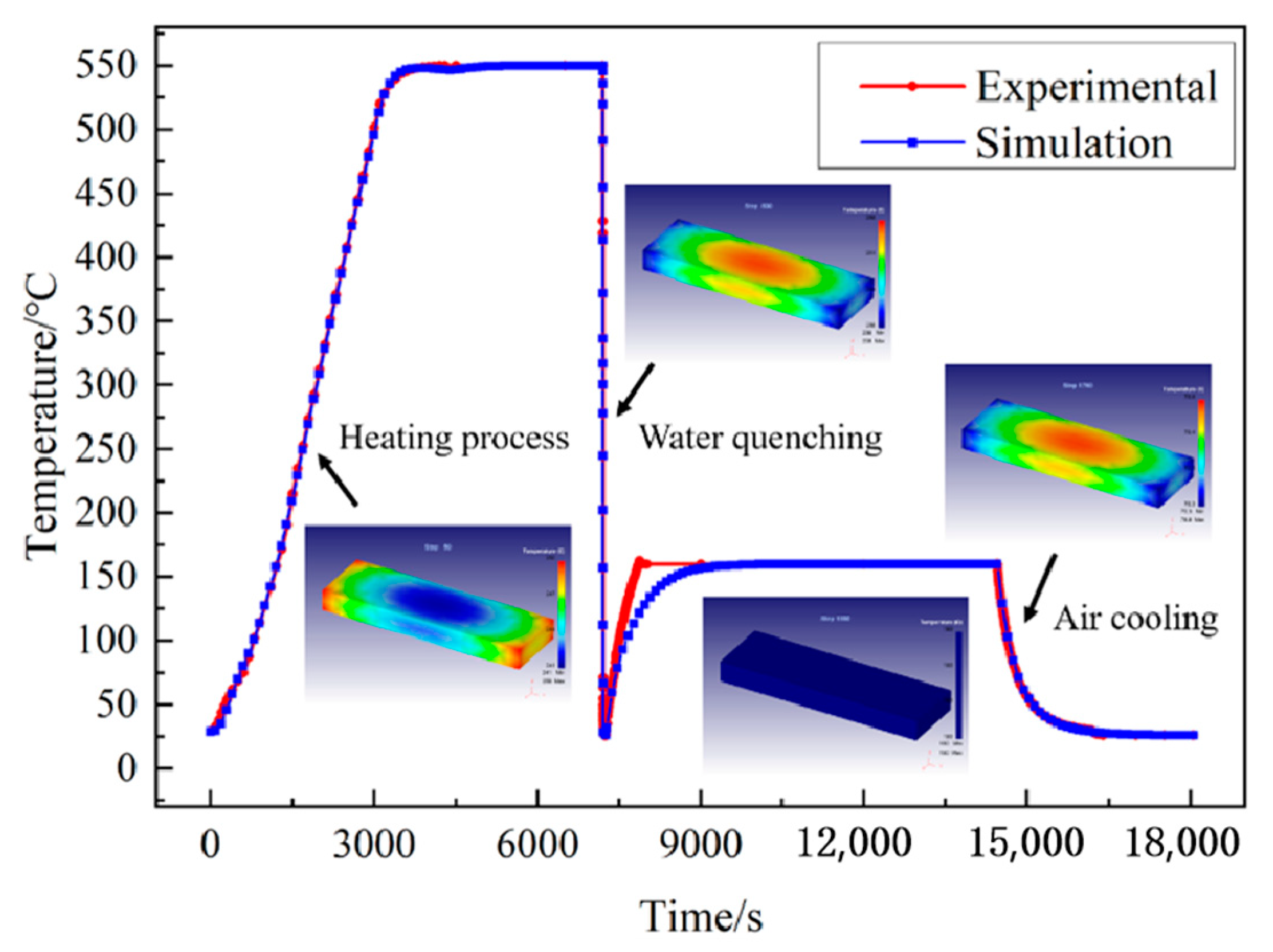
4.4. Simulation of the Entire Heat Treatment Process

The entire heat treatment process of quenching and tempering is simulated in the Heat treatment Wizard module of DEFORM. The comparison between simulated temperature and experimental temperature is shown in Figure 12. As can be seen from the figure, during the whole heat treatment process and air cooling process, the relative error control of experimental temperature and simulation temperature is within 2%. In the water quenching process, only when the time is between 7000–9000 s, the simulated temperature rise is slightly less than the experimental value, and the relative error between the experimental temperature and the simulation temperature is large. The relative error of the other time periods is controlled within 1%. However, throughout the heat treatment process, the simulation temperature curve has the same experimental temperature curve trend and the coincidence degree is high, indicating that the heat transfer coefficient value obtained by the inverse analysis method and the heat treatment simulation are accurate and reliable.
Figure 13 shows the microstructure of samples before and after heat treatment. Figure 13a is the micrograph of the SLM molded parts after polishing and corrosion. In the figure, there are not only a certain number of pores, but also the laser scanning path in the SLM molding process can be clearly seen. Figure 13b shows the microstructure of the workpiece after polishing and corrosion after heat treatment. It can be seen from the figure that after heat treatment, not only the pores are finer and uniform, but the grains are fine, and the precipitated Si tends to be distributed along the grains.

5. Conclusions

For samples prepared with SLM, heat treatment process is needed to improve the performance of the samples. It is very important to obtain accurate heat transfer coefficient for simulating heat treatment process. Combined with the temperature data in the experiment, the heat transfer coefficient of the material under different conditions was calculated by inverse calculation in the reverse heat conduction module in DEFORM. The main conclusions are as follows:
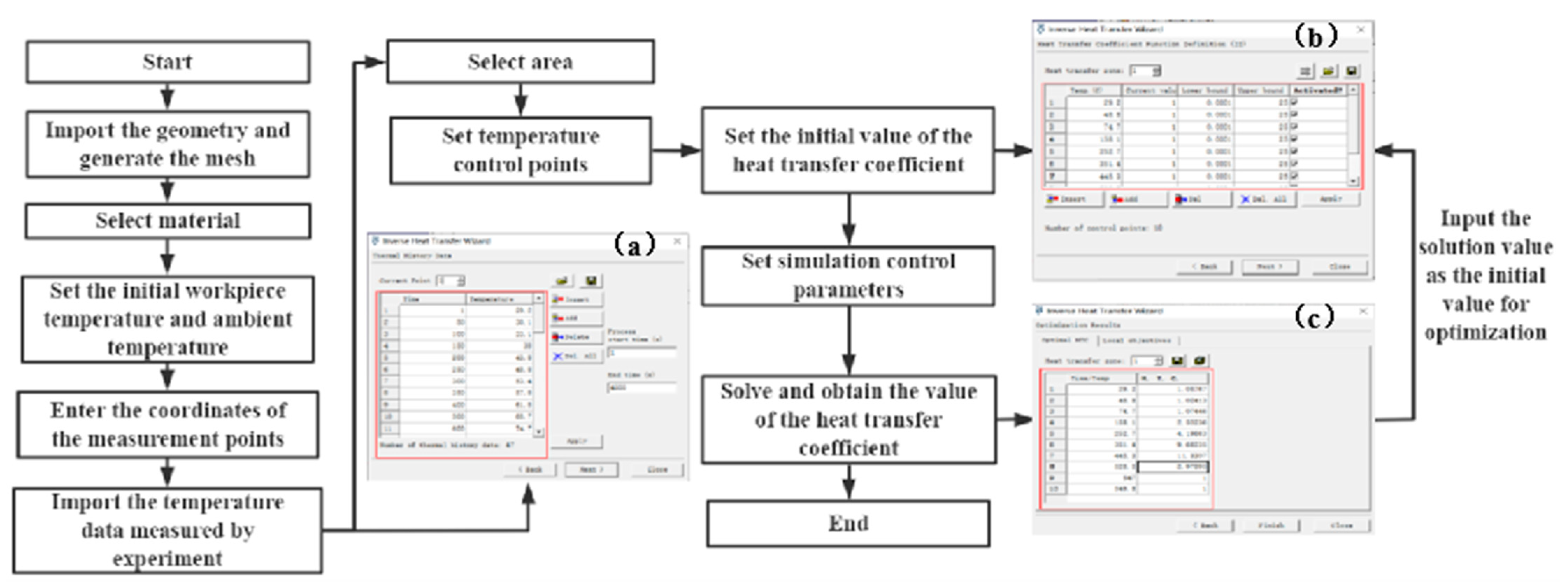
  • Based on the nonlinear evaluation method, the inverse analysis model of heat transfer coefficient in the heat treatment process was established. Taking the actual temperature curve as the input condition, the heat transfer coefficient values of heating, quenching and air cooling parts in the heat treatment process were obtained successfully.
  • In the tempering process, when the temperature is from 100 to 160 °C, the simulated temperature rise is slightly smaller than the experimental value. In the process of temperature drop, the simulation temperature is lower than the experimental value between 42 and 30 °C, while the simulation temperature is slightly higher than the experimental value between 30 °C and room temperature, but the difference is not more than 5 °C.
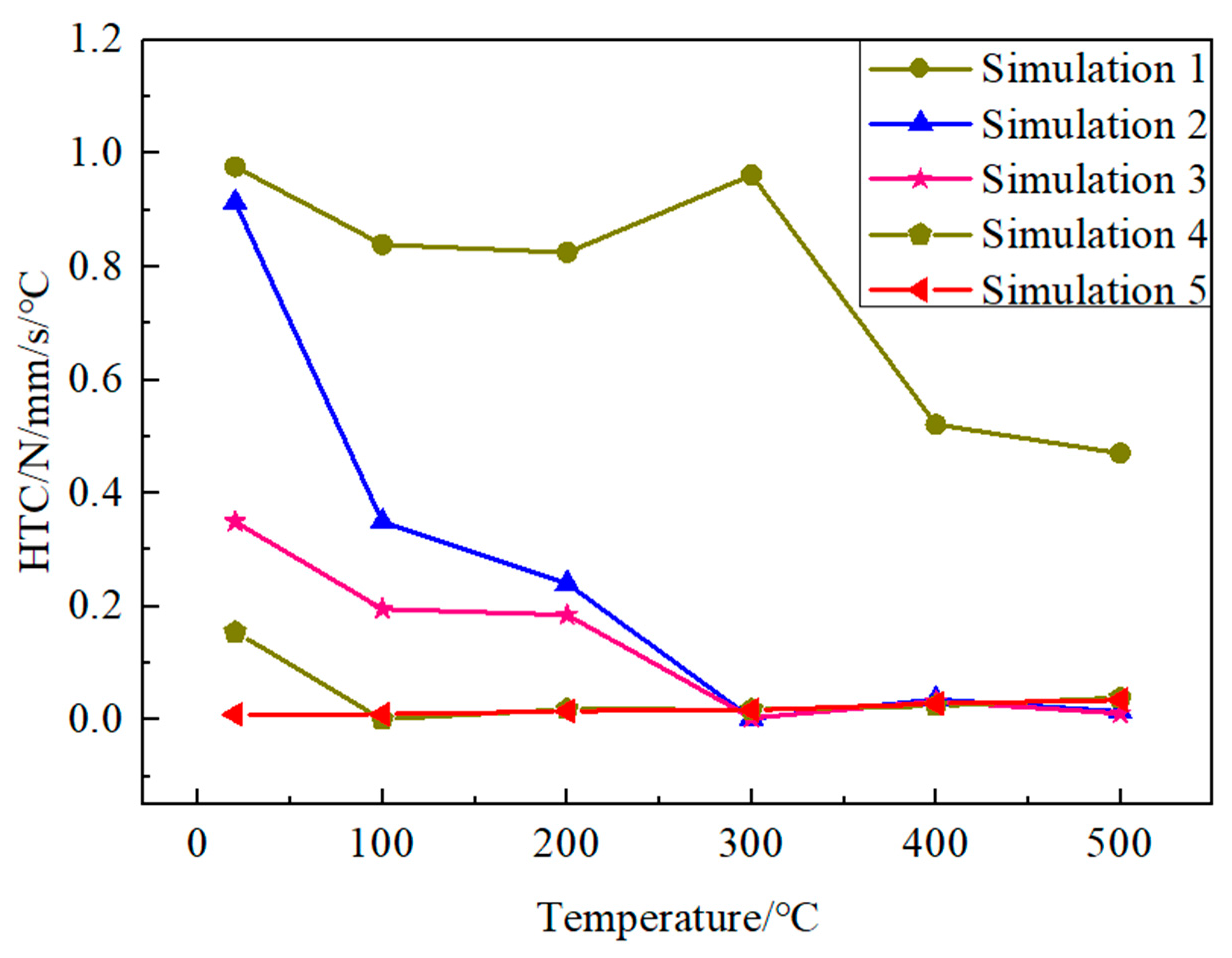
  • The mathematical model of heat transfer coefficient changing with temperature during heat treatment was established.
  • The heat transfer coefficient obtained by the inverse analysis method was used to simulate the heat treatment process, and the obtained simulation temperature curve had a high coincidence degree with the experimental temperature curve.

Author Contributions

Conceptualization, X.J.; Data curation, C.W.; Investigation, W.X., C.L. and Z.L.; Writing—original draft, S.W. All authors have read and agreed to the published version of the manuscript.

Funding

This project is supported by the Natural Science Foundation of China (No.52005098) and the Shanghai Natural Science Foundation (Grant No.20ZR1438000, 22ZR1402400). The authors wish to record their gratitude for their generous supports.

Data Availability Statement

The data and materials that support the findings of this study are available from the corresponding author upon reasonable request.

Acknowledgments

In this section, you can acknowledge any support given which is not covered by the author contribution or funding sections. This may include administrative and technical support, or donations in kind (e.g., materials used for experiments).

Conflicts of Interest

The authors declare no conflict of interest.

References

  1. Luo, H.; Wang, Y.; Zhang, P. Study on Surface Quality of 7A09 Aluminum Alloy Milling Based on Single Factor Method. Surf. Technol. 2020, 49, 327–333. [Google Scholar]
  2. Li, C.; Piao, Y.C.; Meng, B.B.; Hu, Y.; Li, L.; Zhang, F. Phase transition and plastic deformation mechanisms induced by self-rotating grinding of GaN single crystals. Int. J. Mach. Tools Manuf. 2022, 172, 103827. [Google Scholar] [CrossRef]
  3. Wu, C.J.; Li, B.Z.; Liu, Y.; Liang, S.Y. Surface roughness modeling for grinding of Silicon Carbide ceramics considering co-existing of brittleness and ductility. Int. J. Mech. Sci. 2017, 133, 167–177. [Google Scholar] [CrossRef]
  4. Zhang, Y.; Bai, Q.; He, X.; Qing, L.; Yue, S.; Liu, X. Wear analysis of CVD diamond tool in micro-milling AA356 aluminum alloy. Diam. Abras. Eng. 2021, 41, 44–50. [Google Scholar] [CrossRef]
  5. Xing, M.; Lei, X.; Guan, X.; Song, Y.; Zhou, Y. Research on Construction of Super hydro phobic Surface of Aluminum Alloy and Its Stability and Self-cleaning Performance. Surf. Technol. 2021, 50, 152–161. [Google Scholar]
  6. Yan, Y.; Wang, J.; Geng, Y.; Zhang, G. Material Removal Mechanism of Multi-Layer Metal-Film Nanomilling. CIRP Ann.—Manuf. Technol. 2022, 71, 61–64. [Google Scholar] [CrossRef]
  7. Wu, C.J.; Pang, J.Z.; Li, B.Z.; Liang, S.Y. High Speed Grinding of HIP-SiC Ceramics on Transformation of Microscopic Features. Int. J. Adv. Manuf. Technol. 2019, 102, 1913–1921. [Google Scholar] [CrossRef]
  8. Ding, Z.S.; Sun, J.; Guo, W.C.; Jiang, X.; Wu, C.; Liang, S.Y. Thermal Analysis of 3J33 Grinding Under Minimum Quantity Lubrication Condition. Int. J. Precis. Eng. Manuf.-Green Technol. 2021, 91, 1–19. [Google Scholar] [CrossRef]
  9. Xie, Y.; Wang, C.; Zhang, K.; Liang, C.; Liang, C.; Zhou, C.; Lin, D.; Chen, Z. Optimizing Laser Cladding on Aluminum Alloy Surface with Numerical Simulation and Rare Earth Modification. Surf. Technol. 2020, 49, 144–155. [Google Scholar]
  10. Wang, J.Q.; Yan, Y.D.; Li, Z.H.; Geng, Y.Q. Towards understanding the machining mechanism of the atomic force microscopy tip-based nanomilling process. Int. J. Mach. Tools Manuf. 2021, 162, 103701. [Google Scholar] [CrossRef]
  11. Zhu, Y.G.; Wang, Y.G.; Niu, S.W.; Xie, Y.J.; Lei, Y.Y. Effect of environmental friendly complexing agent and oxidant on CMP of aluminium alloy under low pressure. Diam. Abras. Eng. 2020, 40, 74–78. [Google Scholar] [CrossRef]
  12. Guo, W.C.; Wu, C.J.; Ding, Z.S.; Zhou, Q. Prediction of surface roughness based on a hybrid feature selection method and long short-term memory network in grinding. Int. J. Adv. Manuf. Technol. 2021, 112, 1853–2871. [Google Scholar] [CrossRef]
  13. Li, C.; Piao, Y.; Meng, B.; Zhang, Y.; Li, L.; Zhang, F. Anisotropy dependence of material removal and deformation mechanisms during nanoscratch of gallium nitride single crystals on (0001) plane. Appl. Surf. Sci. 2022, 578, 152028. [Google Scholar] [CrossRef]
  14. Sun, Y.; Jin, L.; Gong, Y.D.; Wen, X.L.; Yin, G.; Wen, Q.; Tang, B. Experimental evaluation of surface generation and force time-varying characteristics of curvilinear grooved micro end mills fabricated by EDM. J. Manuf. Processes 2022, 73, 799–814. [Google Scholar] [CrossRef]
  15. Shokoufeh, M.; Krishna, K.; Charbel, A.K.; Jeffrey, R.; Eric, P. Heat transfer simulation and improvement of autoclave loading in composites manufacturing. Int. J. Adv. Manuf. Technol. 2021, 112, 2989–3000. [Google Scholar] [CrossRef]
  16. Su, Y.; Jiang, H.; Liu, Z.Q. An experimental investigation on heat transfer performance of electrostatic spraying used in machining. Int. J. Adv. Manuf. Technol. 2021, 112, 1285–1294. [Google Scholar] [CrossRef]
  17. Kim, D.; Kim, H.; Lee, S. Life Estimation of Hot Press Forming Die by Using Interface Heat Transfer Coefficient Obtained from Inverse Analysis. Int. J. Automot. Technol. 2015, 16, 285–292. [Google Scholar] [CrossRef]
  18. Gianfranco, P.; Vito, P.; Antonio, P. Determination of Interfacial Heat Transfer Coefficients in a Sand Mold Casting Process Using an Optimized Inverse Analysis. Appl. Therm. Eng. 2015, 78, 682–694. [Google Scholar] [CrossRef]
  19. Mikhail, K.; Mikhail, K.; Iuliia, T.; Nikolai, E.S.; Alexey, B. Method for residual strain modeling taking into account mold and distribution of heat transfer coefficients for thermoset composite material parts. Int. J. Adv. Manuf. Technol. 2021, 117, 2429–2443. [Google Scholar] [CrossRef]
  20. Ramos, N.; Mittermeier Christoph Kiendl, J. Experimental and numerical investigations on heat transfer in fused filament fabrication 3D-printed specimens. Int. J. Adv. Manuf. Technol. 2021, 118, 1367–1381. [Google Scholar] [CrossRef]
  21. Kadam, A.R.; Hindasageri, V.; Kumar, G.N. Inverse Estimation of Heat Transfer Coefficient and Reference Temperature in Jet Impingement. ASME J. Heat Transf. 2020, 142, 092302. [Google Scholar] [CrossRef]
  22. Kang, H.C.; Chang, S.M. The Correlation of Heat Transfer Coefficients for the Laminar Natural Convection in a Circular Finned-Tube Heat Exchanger. ASME J. Heat Transf. 2018, 140, 031801. [Google Scholar] [CrossRef]
  23. Piotr, D. Simplification of 3D Transient Heat Conduction by Reducing It to an Axisymmetric Heat Conduction Problem and a New Inverse Method of the Problem Solution. Int. J. Heat Mass Transf. 2019, 143, 118492. [Google Scholar] [CrossRef]
  24. Farzad, M.; Mathieu, S. Estimation of Thermal Conductivity, Heat Transfer Coefficient, and Heat Flux Using a Three Dimensional Inverse Analysis. Int. J. Therm. Sci. 2016, 99, 258–270. [Google Scholar] [CrossRef]
  25. Parida, R.K.; Madav, V.; Hindasageri, V. Analytical Solution to Transient Inverse Heat Conduction Problem Using Green’s Function. J. Therm. Anal. Calorim. 2020, 141, 2391–2404. [Google Scholar] [CrossRef]
  26. Zhang, B.W.; Mei, J.; Cui, M. A General Approach for Solving Three-Dimensional Transient Nonlinear Inverse Heat Conduction Problems in Irregular Complex Structures. Int. J. Heat Mass Transf. 2019, 140, 909–917. [Google Scholar] [CrossRef]
  27. Ming, W.W.; Yu, W.W.; Qiu, K.X.; An, Q.L.; Chen, M. Modelling of the temperature distribution based on equivalent heat transfer theory and anisotropic characteristics of honeycomb core during milling of aluminum honeycomb core. Int. J. Adv. Manuf. Technol. 2021, 115, 2097–2110. [Google Scholar] [CrossRef]
  28. Guo, Z.P.; Xiong, S.M.; Cho, S.H. Heat Transfer between Casting and Die during High Pressure Die Casting Process of AM50 Alloy-Modeling and Experimental Results. J. Mater. Sci. Technol. 2008, 1, 131–135. [Google Scholar] [CrossRef]
  29. Guo, Z.P.; Xiong, S.M.; Liu, B.C. Effect of Process Parameters, Casting Thickness, and Alloys on the Interfacial Heat-Transfer Coefficient in the High-Pressure Die-Casting Process. Metall. Mater. Trans. A Phys. Metall. Mater. Sci. 2009, 39, 2896–2905. [Google Scholar] [CrossRef]
  30. Guo, Z.P.; Xiong, S.M.; Liu, B.C. Determination of the Heat Transfer Coefficient at Metal-Die Interface of High Pressure Die Casting Process of AM50 Alloy. Int. J. Heat Mass Transf. 2009, 51, 6032–6038. [Google Scholar] [CrossRef]
  31. Chen, Y.; Chen, J.H.; Xu, G.D. Screw thermal characteristic analysis and error prediction considering the two-dimensional heat transfer structure. Int. J. Adv. Manuf. Technol. 2021, 115, 2433–2448. [Google Scholar] [CrossRef]
  32. Ho, J.Y.; Leong, K.C.; Wong, T.N. Experimental and numerical investigation of forced convection heat transfer in porous lattice structures produced by selective laser melting. Int. J. Therm. Sci. 2018, 137, 276–287. [Google Scholar] [CrossRef]
  33. Jiang, X.H.; Xiong, W.J.; Wang, Y.F. Heat treatment effects on microstructure-residual stress for selective laser melting AlSi10Mg. Mater. Sci. Technol. 2018, 36, 168–180. [Google Scholar] [CrossRef]
  34. Wang, X.W.; Ho, J.Y.; Leong, K.C. Condensation heat transfer and pressure drop characteristics of R-134a in horizontal smooth tubes and enhanced tubes fabricated by selective laser melting. Int. J. Heat Mass Transf. 2018, 126, 949–962. [Google Scholar] [CrossRef]
  35. Martin, L.; Tobias, M.; Avik, S. Mechanical and thermal characterisation of AlSi10Mg SLM block support structures. Mater. Des. 2019, 183, 108138. [Google Scholar] [CrossRef]
  36. Huiping, L.; Guoqun, Z.; Shanting, N.; Yiguo, L. Inverse heat conduction analysis of quenching process using finite-element and optimization method. Finite Elem. Anal. Des. 2006, 42, 1087–1096. [Google Scholar] [CrossRef]
  37. Kevin, A.; Ryan, F.; Branden, S.; Sawyer, G.; Jake, W.; Saeid, V. Nanofluid Heat Transfer: Enhancement of the Heat Transfer Coefficient inside Microchannels. Nanomaterials 2022, 12, 615. [Google Scholar] [CrossRef]
  38. Khooshehchin, M.; Fathi, S.; Mohammadidoust, A.; Salimi, F.; Ovaysi, S. Experimental study of the effects of horizontal and vertical roughnesses of heater surface on bubble dynamic and heat transfer coefficient in pool boiling. Heat Mass Transf. 2022, 58, 1319–1338. [Google Scholar] [CrossRef]
  39. James, V.B. Transient Sensitivity Coefficients for the Thermal Contact Conductance. Int. J. Heat Mass Transf. 1967, 10, 1615–1617. [Google Scholar] [CrossRef]
  40. Beck, J.V.; Litkouhi, B.; Clair, C.R. Efficient Sequential Solution of the Nonlinear Inverse Heat Conduction Problem. Numer. Heat Transf. 1982, 5, 275–286. [Google Scholar] [CrossRef]
  41. Beck, J.V. Combined Parameter and Function Estimation in Heat Transfer with Application to Contact Conductance. ASME J. Heat Transf. 1988, 110, 1046–1058. [Google Scholar] [CrossRef]
Figure 1. Space M200 manufacturing system.
Crystals 12 01309 g001
Figure 2. The process of heat treatment temperature measurement.(a) The SLM printing equipment. (b) The size of the AlSi10Mg sample. (c) The thermocouple is inserted into a small hole on the surface of the sample to measure and obtain the temperature data during the heat treatment process in real time. (d) The comparison curve of the measured temperature and the simulated temperature.
Crystals 12 01309 g002
Figure 3. Heat flux solved by discrete solution. (a) The actual heat flux q t is dispersed into a series of values. (b) The heat flux is assumed to be constant in the R Δθ time.
Crystals 12 01309 g003aCrystals 12 01309 g003b
Figure 4. The process of solving the heat transfer coefficient in DEFORM.
Crystals 12 01309 g004
Figure 5. Stages of heat treatment.
Crystals 12 01309 g005
Figure 6. Temperature curve in the heating process.
Crystals 12 01309 g006
Figure 7. The heat transfer coefficient curve in the heating process.
Crystals 12 01309 g007
Figure 8. Fitting curve of heat transfer coefficient in the heating process.
Crystals 12 01309 g008
Figure 9. Temperature and heat transfer coefficient curves during quenching. (a) Comparison between the experimental temperature and the simulation temperature of point 1. (b) Comparison between the experimental temperature and the simulation temperature of point 2. (c) Comparison between the experimental temperature and the simulation temperature of point 3.
Crystals 12 01309 g009
Figure 10. Fitting curve of heat transfer coefficient during quenching.
Crystals 12 01309 g010
Figure 11. Comparison between the simulation and experiment of the temperature drop process during air cooling.
Crystals 12 01309 g011
Figure 12. Comparison of the simulation and experimental temperatures in the heat treatment process.
Crystals 12 01309 g012
Figure 13. Microstructure of samples before and after heat treatment. (a) Micrograph of SLM molding parts. (b) micrograph of workpiece after heat treatment.
Crystals 12 01309 g013
Table 1. Chemical composition of AlSi10Mg alloy powder (wt.%).
AlSiMgFeNOTi
Bal9.0–110.25–0.45<0.25<0.2<0.2<0.15
ZnMnNiCuPbSn
<0.1<0.1<0.05<0.05<0.02<0.02
Table 2. Thermophysical parameters of AlSi10Mg alloy.
Temperature, T/°C20100200300400
Thermal conductivity, K s w m ° C 147155159159155
Specific heat capacity, C J kg ° C 739755797838922
Density, ρ kg / m 3 2650
Table 3. Mechanical property parameters of AlSi10Mg alloy material.
Temperature, T/°C20100200300400
Modulus of elasticity, E E GPa 6967625341
The yield strength, σ s MPa 1951501057030
Coefficient of thermal expansion, θ 10 6 ° C 21.722.523.523.325.5
Poisson’s ratio, μ 0.33
Table 4. The parameters of the simulation part.
Number of ElementsControl PointsTime per StepStep Increm-Ent to SaveRelative Improve-Ment Less Than (%)Maximum IterationsMaxi-Mum Simula-TionsObjective Function Less ThanDecision Vector Change Less Than
200030.0110250050001 1 × 10 6
Table 5. The temperature data of the heating progress.
Time/sExperimentalSimulation 1Simulation 2Simulation 3Simulation 4Simulation 5
129.228.996128.996228.997828.998828.9999
5030.130.880430.860530.431429.940729.1261
10033.139.281839.182237.297434.650429.9117
1503855.468155.167151.782545.579532.1536
20043.871.904671.469867.939658.695636.1405
25048.885.994485.493882.265670.376741.4023
30053.497.68197.154494.29579.774947.4175
35057.8106.393105.972103.70986.841453.7204
40061.8112.949112.636110.90791.884359.9506
50068.7121.182120.98119.90897.738871.4138
60074.7126.145126.026125.385100.38181.2586
70087.3145.922145.331142.338103.291.0137
800102.2170.45169.73166.104108.093102.4
900114.1184.481184.086182.064115.227115.351
1100142214.063213.599210.909136.221144.012
1200158.1232.317231.738227.384151.1159.98
1300171.7242.423242.13239.072168.628176.39
1400190.6263.318262.636254.466188.727193.41
1500214.7283.373282.751271.081211.848212.16
1600235.1304.382303.697285.267235.064232.251
1700252.7317.692317.118294.642256.976252.496
1800273.6336.086334.808299.937277.56272.462
1900292.5351.39349.847304.769297.45292.42
2000312.2368.234365.431312.512316.487312.094
2100331.6384.614379.915324.467335.035331.884
2200351.4401.144392.131341.607353.16351.586
2300370.5417.059399.861363.754370.914371.027
2400390.1434.291406.531389.339388.563390.36
2500408.2449.59416.156414.394406.084409.341
2600427.2466.5428.51435.182424.268427.89
2700445.3481.756443.328453.561443.048446.114
2800464.4497.148459.974470.534461.961463.942
2900483.1511.61478.084486.896480.97481.63
3000501.8524.546496.99502.794499.804499.101
3100520534.75516.088518.288518.252516.28
3200528.5539.852530.897530.215532.182529.585
3300535.7541.867539.516537.492540.162537.681
3400539.8542.971544.474542.138544.754542.695
3500543.3543.58546.988544.905547.094545.545
3600545.4543.975548.188546.552548.219547.129
3700547544.223548.571547.407548.578547.862
3800548544.4548.587547.819548.59548.146
3900548.7544.524548.353547.903548.359548.112
4000549.3544.613547.958547.756547.969547.864
4100549.6544.675547.494547.469547.51547.5
4200549.8544.721547.016547.111547.034547.085
4300549.8544.751546.527546.702546.548546.636
The temperature data at a certain time obtained by the experiment can be input into the above formula to obtain the corresponding heat transfer coefficient value, which can be used in the subsequent heat treatment process simulation
Table 6. Heat transfer coefficient values obtained during the fifth simulation.
Temperature/°C20100200300400500
Heat transfer coefficient/
N/mm·s·°C
111.541.732.893.54
The temperature data at a certain time obtained by the experiment can be input into the above formula to obtain the corresponding heat transfer coefficient value, which can be used in the subsequent heat treatment process simulation
Table 7. Heat transfer coefficient values obtained in the third simulation.
Temperature/°C20100200300400500
Heat transfer coefficient/
N/mm·s·°C
4.243.546.030.600.854.87
Table 8. Simulated heat transfer coefficient values during air cooling.
Temperature/°C20100200
Heat transfer coefficient/
N/mm·s·°C
111
Publisher’s Note: MDPI stays neutral with regard to jurisdictional claims in published maps and institutional affiliations.

