Predicting Flow Stress Behavior of an AA7075 Alloy Using Machine Learning Methods

Abstract

The present work focuses on the prediction of the hot deformation behavior of thermo-mechanically processed precipitation hardenable aluminum alloy AA7075. The data considered focus on a novel hot forming process at different tool temperatures ranging from $24{}^{\circ }$C to $350{}^{\circ }$C to set different cooling rates after solution heat-treatment. Isothermal uniaxial tensile tests in the temperature range of $200{}^{\circ }$C to $400{}^{\circ }$C and at strain rates ranging from 0.001 s${}^{-1}$ to 0.1 s${}^{-1}$ were carried out on four different material conditions. The present paper mainly focuses on a comparative study of modeling techniques based on Machine Learning (ML) and the Zerilli–Armstrong model (Z–A) as reference. Related work focuses on predicting single data points of the curves that the model was trained on. Due to the way data were split with respect to training and testing data, it is possible to predict entire stress–strain curves. The model allows to decrease the number of required laboratory experiments, eventually saving costs and time in future experiments. While all investigated ML methods showed a higher performance than the Z–A model, the extreme Gradient Boosting model (XGB) showed superior results, i.e., the highest error reduction of 91% with respect to the Mean Squared Error.

1. Introduction

Lightweight parts of aluminum (Al) alloys are widely used in the automotive industry to replace heavy steel parts in order to reduce the weights of components. This design concept allows for a reduction in fuel consumption and carbon dioxide emissions [1,2]. Among precipitation-hardenable, high-strength aluminum alloys, AA7075-T6 alloy with its high ultimate strength (UTS) was found to be a promising candidate to be a steel substitute [3,4]. Recently, the combination of AA7075 with hot forming processes led to promising results [5,6,7]. However, the desire for trustworthy data to be employed for estimation of the necessary forces implemented during hot forming of AA7075 alloy has prompted interest in its elevated temperature behavior, especially its flow stress behavior [4,8,9,10,11]. These data can be obtained via experiments such as tensile tests at elevated temperatures, but due to the numerous parameters (strain rate, deformation temperature, atmospheric conditions, etc.) affecting the resulting mechanical properties, these experiments are time consuming and expensive. To reduce the number of experiments, and time and cost, researchers and engineers have been trying to predict the flow stress behavior in the form of stress–strain curves for decades, focusing on different deformation conditions (i.e., various temperatures and strain rates) [4,12,13,14,15,16,17,18]. Techniques for the prediction of the flow stress behavior of alloys at elevated temperatures can be classified as physically-based [12,13,15], phenomenological [16] and data-driven [17,18,19,20,21]. All three modeling approaches were used to predict the mechanical behavior of different Al alloys at elevated temperatures [4,7,17,18].

Physically-based models predict the behavior of materials based on changes in their microstructure imposed by the deformation at elevated temperatures. The prediction of stress–strain curves of materials via physically-based modeling techniques with high accuracy is challenging due to the high number of micro- and macroscopic parameters needed to predict the flow behavior of the material. Forming AA7075 at elevated temperatures may lead to the occurrence of softening mechanisms, i.e., dynamic recovery (DRV) and dynamic recrystallization (DRX) [6,8]. Additionally, the occurrence of necking should also be taken into account for the prediction of flow stress curves under tensile loading. Therefore, an accurate modeling with a physically-based modeling technique is very complex. In order to evaluate an alternative approach, the focus of the present work is data-driven Machine Learning (ML) based models.

Phenomenological and empirical models such as the Johnson–Cook (J–C) equation, the Zerilli–Armstrong (Z–A) and the Arrhenius-type models only take macroscopic deformation factors into account [16]. Thus, these models do not consider the microstructural evolution of materials such as changes in the dislocation densities during the tensile test. Similar to the physically-based models, the prediction of stress–strain curves of materials via those modeling techniques is challenging when high accuracy is desired. The J–C equation was used to simulate the mechanical properties of AA7075 in T6 condition at temperatures ranging from $25{}^{\circ }$C to $600{}^{\circ }$C and strain rates of 5 × 10${}^{-4}$ s${}^{-1}$ to 800 s${}^{-1}$ [4]. In another study, a modified J–C model was utilized to predict the flow stress response of AA7075 alloy at $350{}^{\circ }$C to $450{}^{\circ }$C and at strain rates of 0.001 s${}^{-1}$ to 0.1 s${}^{-1}$ [7]. The results of both studies revealed that J–C can simulate the mechanical behavior of AA7075 alloy with acceptable accuracy.

Due to the steady increase in computing power in recent years and the versatility of ML methods, data-driven models have also been used to predict the behavior of materials at elevated temperatures [17,18,19,20,21]. The main concept of data-driven modeling is to find correlations between variables of system state (input and output) without having an explicit understanding of the physical behavior of the system. Among other data-driven models Artificial Neural Networks (ANN), e.g., the Multi-Layer Perceptron (MLP) were found to be capable of modeling the mechanical properties of alloys at high temperatures with high accuracy [22,23,24,25,26]. In the study of Li et al. [18], an MLP model resulted in the lowest error compared to other models such as a phenomenological Arrhenius-type model and the physically-based Estrin and Mecking equation employed for the prediction of stress–strain curves of homogenized AA6082 alloy at temperatures of $380{}^{\circ }$C to $530{}^{\circ }$C and strain rates of 0.01 s${}^{-1}$ to 10 s${}^{-1}$. Moreover, Haghdadi et al. [17] studied the accuracy of MLP modeling for the hot deformation of a cast A356 aluminum alloy at $400{}^{\circ }$C to $540{}^{\circ }$C under strain rates of 0.001 s${}^{-1}$, 0.01 s${}^{-1}$ and 0.1 s${}^{-1}$.

Besides MLP, other ML methods were used in some recent studies to predict flow stress behavior. Song [22] and Desu et al. [27] predicted the flow stress of austenitic stainless steels based on the inputs of strain, strain rate, and deformation temperature using Support Vector Machines (SVM). The SVM outperformed not only classical mathematical models but also ANN in terms of reliability, predictability, and speed [22,27]. Song [28] also carried out an investigation on stainless steels during hot deformation at temperatures of $700{}^{\circ }$C to $900{}^{\circ }$C under strain rates from 0.0002 s${}^{-1}$ to 0.02 s${}^{-1}$ using the Random Forest (RF) approach. All studies mentioned above have in common that no predictions of complete stress–strain curves have been made. This means that the ML models were used to predict single data points of trained curves. This has the consequence that the models generalization capability is poor, i.e., a transfer to new and so far unknown curves is not possible.

The present study aims to provide a model that predicts the flow stress behavior of thermo-mechanically processed AA7075 alloy for curves, which are explicitly not in the training dataset available. The thermo-mechanical process used in the present study is a novel hot forming process combining solution heat-treatment, forming and die quenching. The process leads to unique mechanical properties of the AA7075 alloy [5,29]. At first, this study investigates if it is generally possible to model the hot deformation behavior of the thermo-mechanically processed precipitation-hardenable aluminum alloy AA7075 with reasonable accuracy. For this purpose, the empirical Z–A model is compared to different ML methods. Moreover, it was investigated whether it is feasible to use ML methods to predict true stress–strain curves with parameter combinations outside the training parameter space. The objective of the ML methods employed is to predict complete curves with parameter combinations that are unknown to the model. Providing models that can predict curves outside the training parameter space allows addressing practical, real-world challenges to reduce the number of tensile tests required and still predict the flow stress behavior over a wide range of parameters.

2. Materials and Methods

In this section, the data used for assessment are presented. Moreover, the modeling approach employed for the prediction of the flow stress behavior is explained. To allow for meaningful comparison, the mathematical derivation of the empirical based Z–A model is shown in detail. In addition, the evaluation procedure further referred to as “data processing pipeline” is explained. The different ML-methods used in the data processing pipeline will be briefly introduced at the end of this chapter.

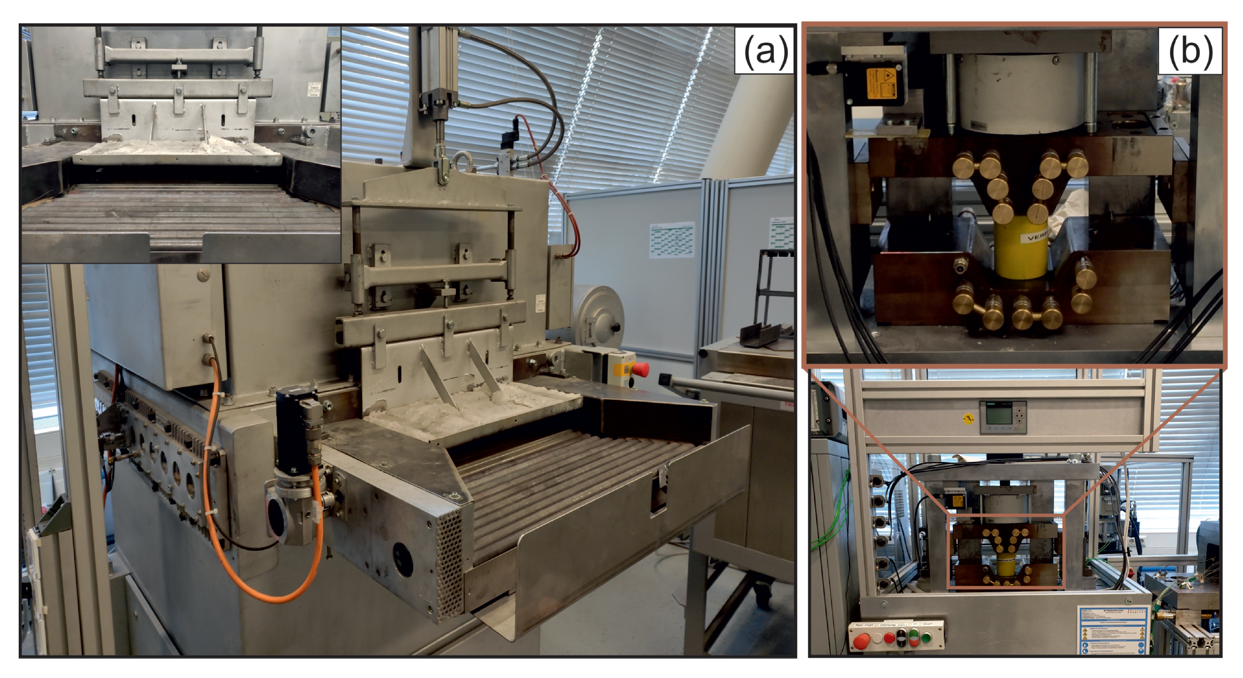
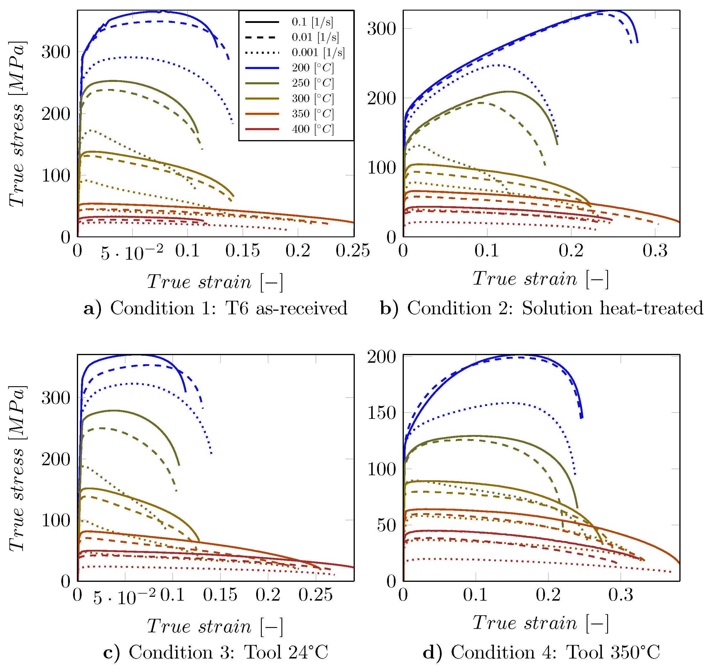
2.1. Data and Experimental Setup

To model the flow stress behavior, data of tensile tests at elevated temperatures of thermo-mechanically processed samples of AA7075 alloy were used. The samples were produced using different thermo-mechanical treatments and the tensile experiments were performed under different deformation temperatures T and strain rates $\dot{ϵ}$. The thermo-mechanical treatments, the corresponding microstructural evolution and the results of the tensile experiments are comprehensively explained in a previous work published by some of the authors of the present paper [5,29,30,31]. As initial condition sheets of AA7075 alloy with the chemical composition listed in

Table 1. Chemical composition of investigated AA7075 alloy experimentally determined using optical emission spectroscopy (OES).

Element	Si	Fe	Cu	Mn	Mg	Cr	Zn	Ti	Zr	Al
AA7075 (Wt.- %)	0.10	0.11	1.59	0.03	2.38	0.20	5.57	0.03	0.04	Balanced

were used.

The production of samples for tensile experiments was performed in subsequent steps as shown in Figure 1. As displayed in Figure 1a, the roller hearth furnace was employed for the solution heat-treatment of the AA7075 sheets. The heatable forming tool used in the present study can be seen in Figure 1b. After solution heat-treatment at $480{}^{\circ }$C for 5 min, the sheets of AA7075 alloy were formed in tools at temperatures of $24{}^{\circ }$C and $350{}^{\circ }$C, respectively. Using two different tool temperatures, the impact of tool temperature on the hot deformation characteristics and modeling of flow curves could be assessed. Following this forming process, all produced profiles were subsequently aged at $120{}^{\circ }$C for 24 h to avoid any subsequent natural aging.

In total, four different conditions were considered in the tensile tests: as received (referred to as T6 in the following), solution heat-treated, solution heat-treated subsequently formed in a tool with a temperature of $24{}^{\circ }$C (referred to as Tool $24{}^{\circ }$C in the following) and solution heat-treated subsequently formed in a tool with a temperature of $350{}^{\circ }$C (referred to as Tool $350{}^{\circ }$C in the following). Tensile samples with a gauge length of 40 mm were cut from the bottom of the produced profiles of all four conditions using electrical discharge machining (EDM). Grinding was employed to remove any residue stemming from EDM before tensile testing. Tensile experiments were carried out at deformation temperatures of $200{}^{\circ }$C, $250{}^{\circ }$C, $300{}^{\circ }$C, $350{}^{\circ }$C and $400{}^{\circ }$C under strain rates of 0.001 s${}^{-1}$, 0.01 s${}^{-1}$ and 0.1 s${}^{-1}$. In consequence, 15 curves are available for each of the examined conditions and therefore a total of 60 curves are provided for the basis of the present study. During the experiments, temperatures and elongation were controlled utilizing thermocouples and extensometers, respectively. The resulting stress–strain curves are shown in Figure 2 and will be explained in the following.

2.1.1. Condition 1: T6 As-Received (Figure 2a)

The mechanical properties of AA7075 in the T6 condition are very sensitive to the deformation temperature and strain rate. With an increase in the deformation temperature or reduction in the strain rate, the strength of the T6 condition is significantly reduced, revealing the occurrence of softening mechanisms at elevated temperatures [5].

2.1.2. Condition 2: Solution Heat-Treated (Figure 2b)

Flow stress levels of solution heat-treated samples were also sensitive to deformation temperature and strain rate. However, a noticeable work hardening can be seen for the solution heat-treated samples deformed at $200{}^{\circ }$C and $250{}^{\circ }$C. This can be rationalized by the onset of dynamic precipitation in the thermally unstable condition. Further heating and simultaneous forming of the solution-heat-treated samples during elevated temperature tensile testing eventually leads to the formation of second phase precipitates and subsequent growth of those features [5].

2.1.3. Condition 3: Tool 24 ${}^{\circ }$C (Figure 2c)

The parts formed and quenched in the tool with the temperature of $24{}^{\circ }$C showed high UTS similar to the T6 conditions [5] due to fine and dispersed precipitates with low interparticle spacing. These precipitates form during the thermo-mechanical treatment imposed by the high cooling rate in forming and quenching of the parts, promoting the evolution of a supersaturated condition being the optimal basis for subsequent aging treatment. The precipitates interact with moving dislocation upon plastic deformation of the alloy leading to high UTS [29].

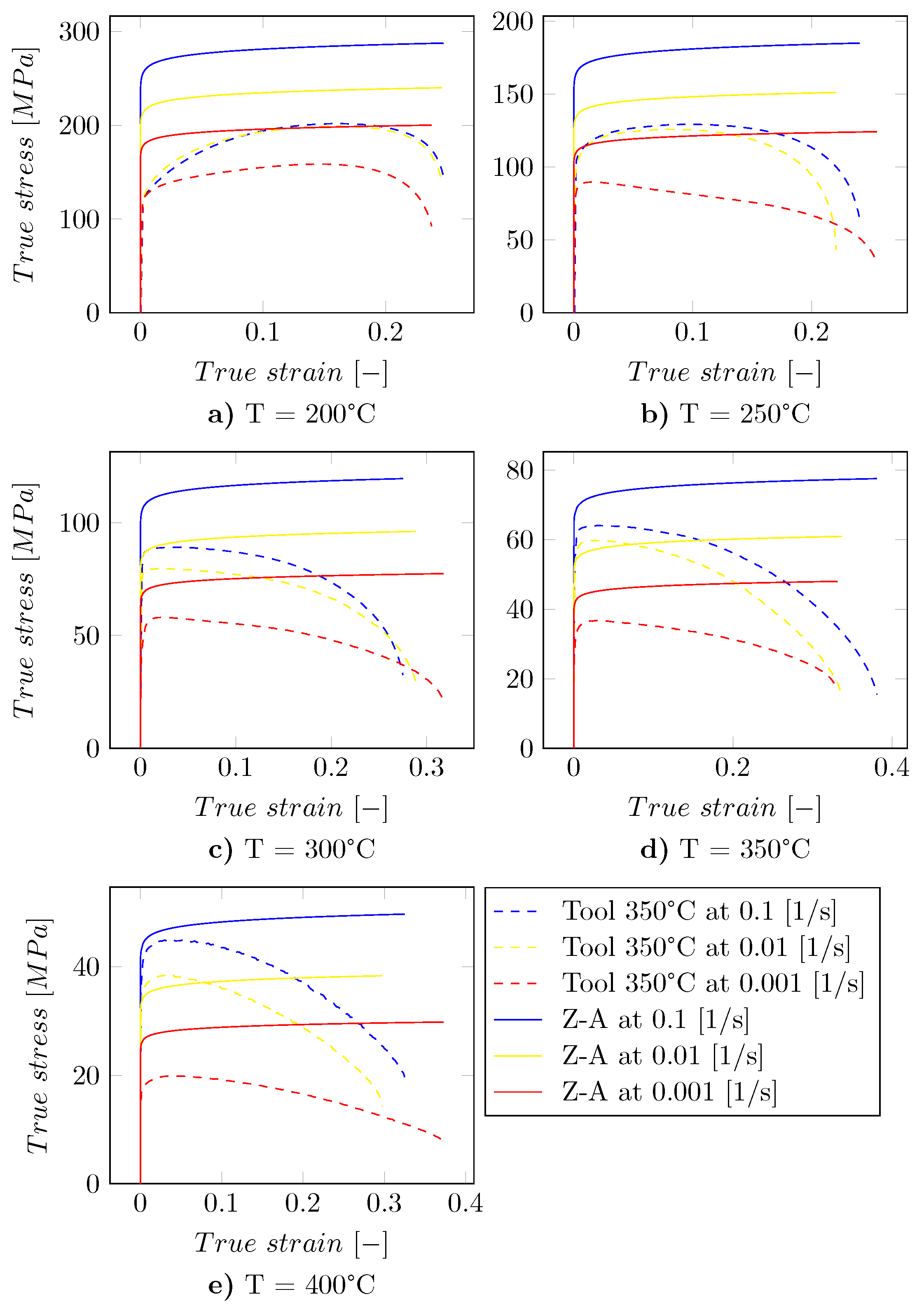
2.1.4. Condition 4: Tool 350 ${}^{\circ }$C (Figure 2d)

It was previously reported that hot forming and quenching of AA7075 in the tool with a temperature of $350{}^{\circ }$C results in low tensile strength at different temperatures [5]. The reason for this material behavior is linked to the non-optimal precipitate size and morphology. At this point, the issue is the low cooling rate in forming and quenching of the parts processed in the hot tool. Coarse precipitates form that do not have a significant strengthening effect [29].

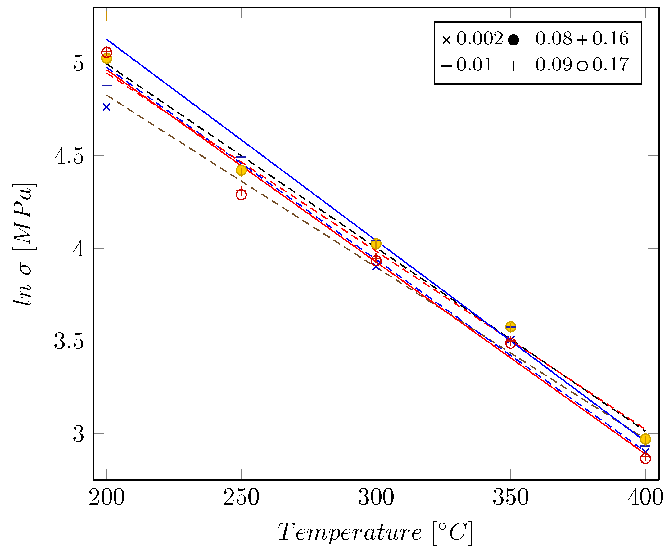
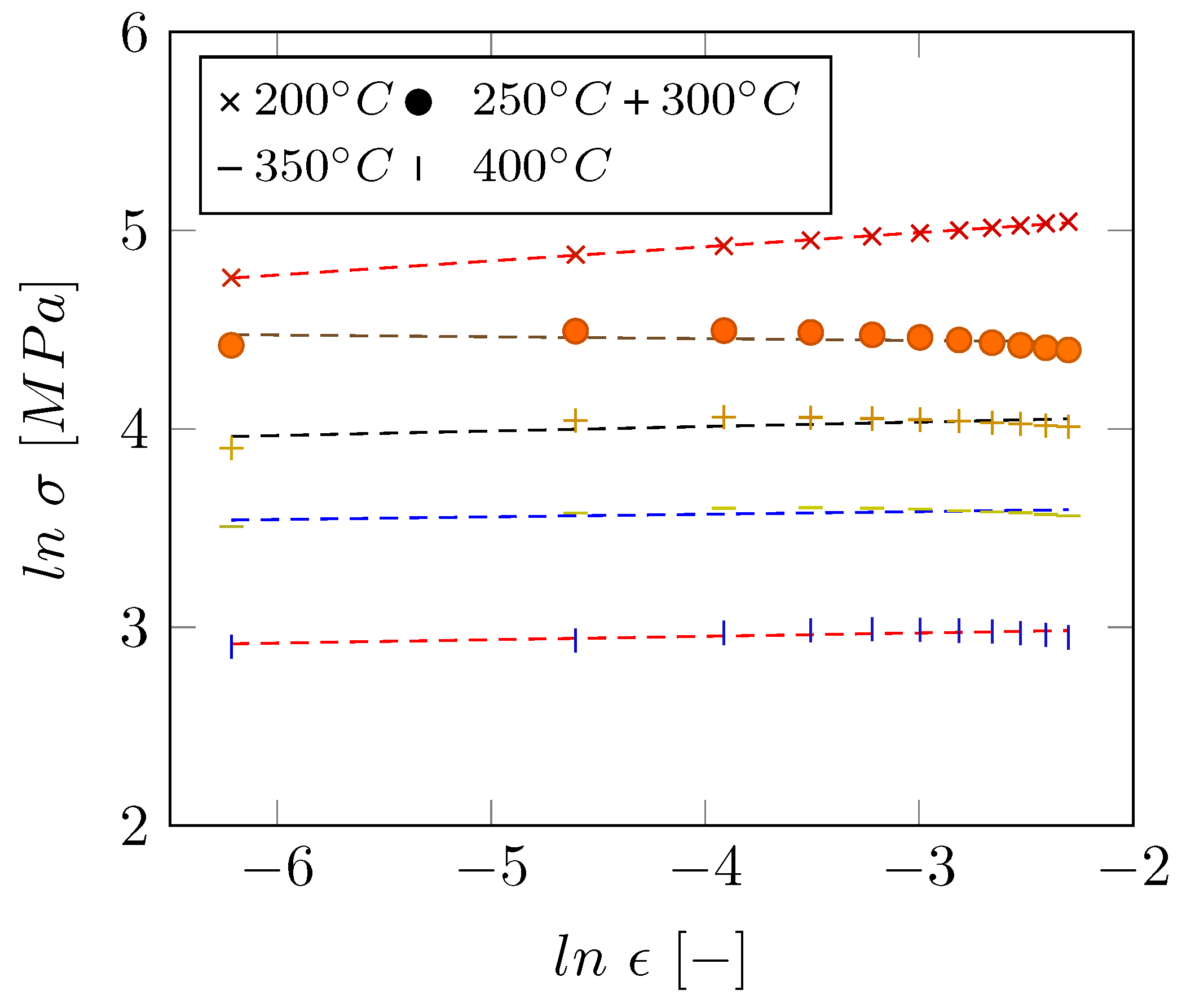
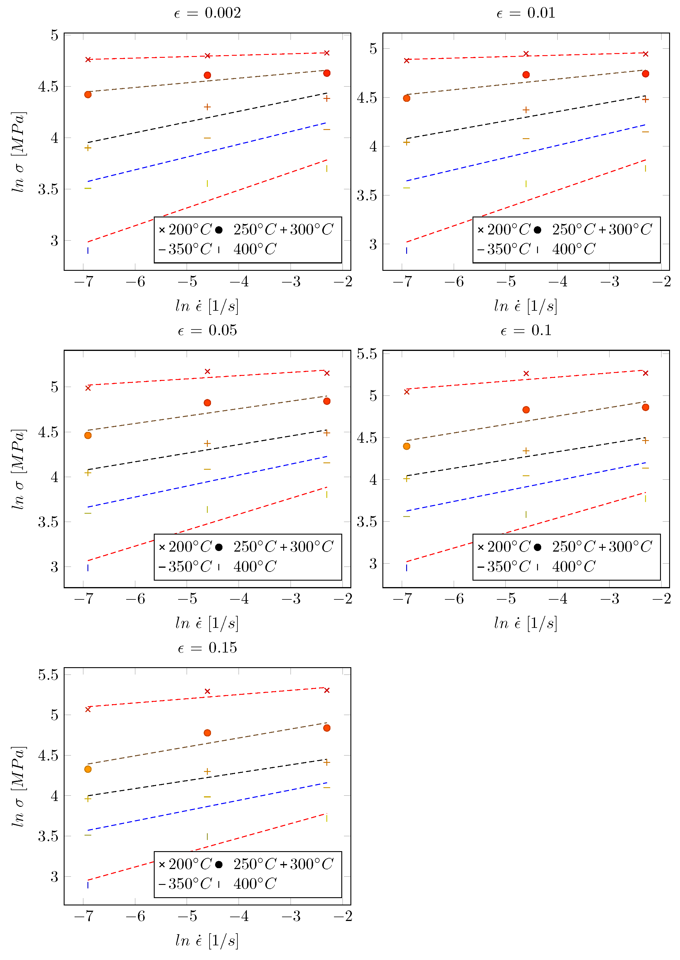
2.2. Zerilli–Armstrong Model

An empirical model based on the Zerilli–Armstrong (Z–A) constitutive equation [12,15] is employed to predict the elevated temperature tensile behavior of the AA7075 alloy. Here, the stress $\sigma$ is calculated based on the strain $ϵ$, the strain rate $\dot{ϵ}$, the temperature T and the material constants $B_0$, n, ${\beta }_0$ and ${\beta }_1$ using:

$$\sigma =B_0{ϵ}^{n}exp(-{\beta }_{0}T+{\beta }_{1}Tln\dot{ϵ}).$$

(1)

The above equation can be simplified as:

$$ln\sigma =ln{B}_0+nlnϵ-({\beta }_0-{\beta }_{1}ln\dot{ϵ})T.$$

(2)

For the sake of brevity, only modeling results of one of the conditions, i.e., thermo-mechanically processed material in the tool with a temperature of $350{}^{\circ }$C are reported, as these have shown the best agreement between the model and experimental data. In order to obtain $B_0$, a reference strain rate of 0.001 s${}^{-1}$ was considered to simplify the equation in the beginning and calculate the first material constant.

By consideration of a reference strain rate, the term $-({\beta }_0-{\beta }_{1}ln\dot{ϵ})$ can be assumed to be constant, named C in the following. Hence, C can be calculated from the slopes of $ln\sigma$ versus deformation temperature in Kelvin at a given strain as shown in Figure 3. Here, it can be deduced that C is independent of strain since the fitting lines are parallel with each other and their slopes hardly vary with changes in strain values. The average value of the slopes was found to be $-0.0101$ K${}^{-1}$. According to Equation (2), the n values can also be determined from the slope of $ln\sigma$ versus $lnϵ$ at a constant temperature as displayed in Figure 4. The average n value was obtained to be 0.025 MPa. Furthermore, the intercepts of fitted lines in the plot $ln\sigma$ versus $lnϵ$ are equal to $ln{B}_0+0.0101T$. So, the $B_0$ values can be obtained at each deformation temperature. The average value $B_0$ was calculated to be 19,250.144 MPa.

As displayed in Figure 5, material constants of ${\beta }_0$ and ${\beta }_1$ can also be determined from the intercepts and slopes of fitted lines in the $ln\sigma$ versus $ln\dot{ϵ}$ plot at various strain values, respectively. The average values for ${\beta }_0$ and ${\beta }_1$ were calculated as 0.008428 K${}^{-1}$ and 0.000166 K${}^{-1}$, respectively.

By substituting all the material constants in Equation (1), the Z–A constitutive equation for AA7075 alloy formed in the tool with a temperature of $350{}^{\circ }$C can be obtained as:

$$\sigma =19250.144{ϵ}^{0.025}exp(-0.000166T+0.008428Tln\dot{ϵ}).$$

(3)

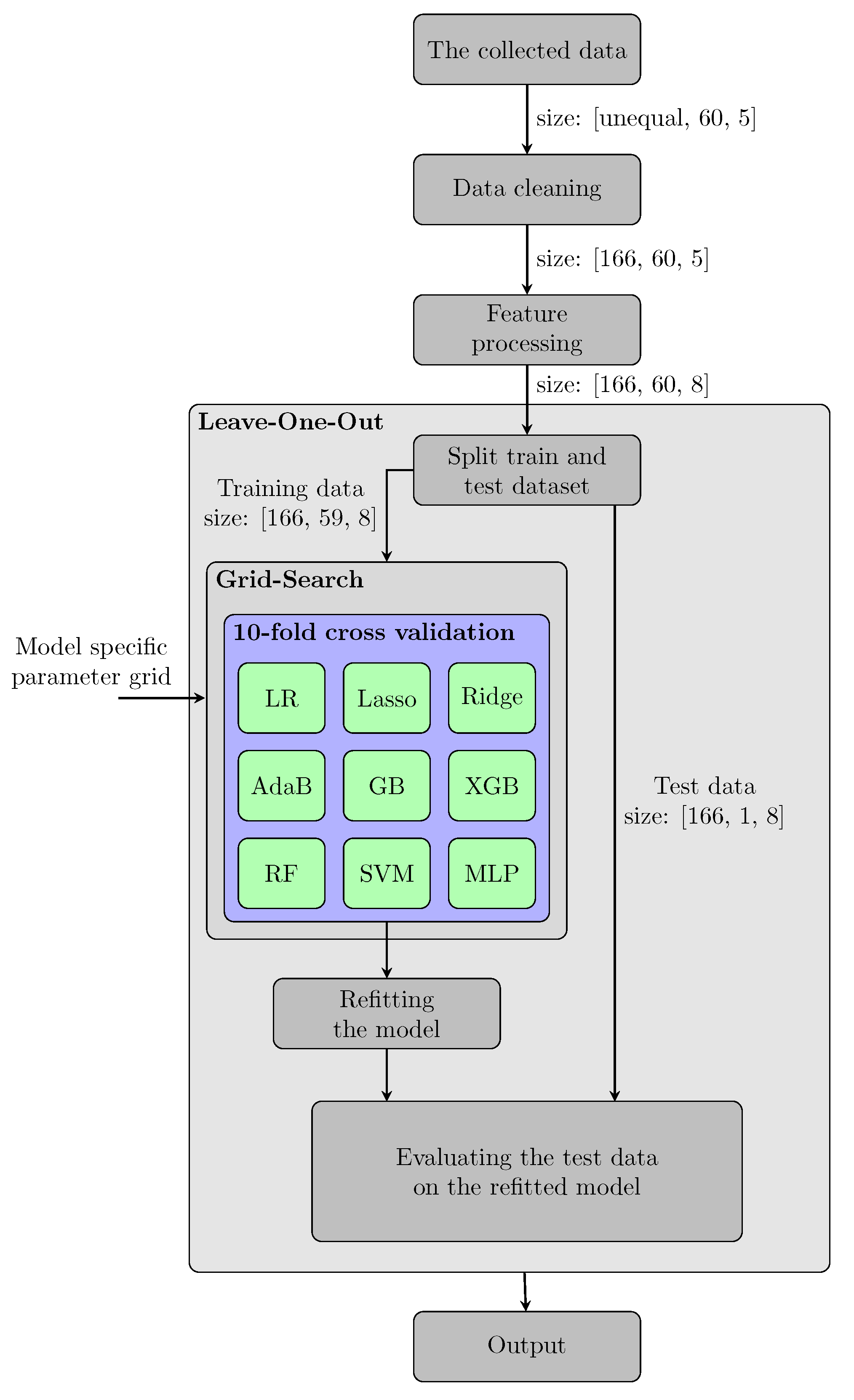
2.3. Machine Learning Methods

Before the ML methods used in this study are introduced, the data processing pipeline is presented. A pipeline is a procedure for automating the workflows required to build a ML model. ML pipelines consist of several sequential steps, ranging from data extraction and preprocessing to model training and deployment. In Figure 6 the schematic representation of the general data preparation and preprocessing procedure of the data processing pipeline is shown.

Exclusively supervised machine learning methods are used, which means that an input to an output is mapped based on a training set consisting of input-output pairs. As mentioned before, 60 curves were obtained in previous studies by tensile tests [5]. Every true stress–strain curve is referred to as one dataset in the following. Each dataset has four features: condition, temperature, strain-rate, true strain, and one target value: true stress. During data cleaning, the experimentally determined datasets are first adjusted to a uniform number of samples in each dataset. The reason for different dataset sizes is that the extensometer records data at a constant data acquisition rate. Therefore, the number of data points recorded varies depending on the time until failure. The dataset with the least number of data points consisted of 166 points. Therefore, the other 59 datasets are reduced to this number during the data cleaning step. The points that are kept are selected to be equidistant considering true strain. Consequently, the actual curve still qualitatively represents the same, however, using fewer data and lower resolution, respectively.

After data cleaning, the nominal feature condition is one-hot encoded. In one-hot encoding, the feature is represented in binary form. Since the feature condition has four attributes, the feature space is increased by three features in order to enable a binary representation. These features are mutually exclusive.

After feature processing, a leave-one-out analysis is executed. For the leave-one-out method, a regression method is applied to 59 datasets and tested for each remaining dataset. This process is repeated 60 times. Therefore, a new model is determined for each dataset. The quality of the leave-one-out study is evaluated by the mean and variance of the $Skill$ score of the 60 observations. In this way, it was ensured that for validation the actual testing data never have been seen by the models before.

To model the elevated temperature tensile behavior, a total of nine model classes from four different model categories are used in the pipeline. These categories are shown in

Table 2. Hyperparameters of ML methods being used in this present work.

Categories	Model	Source	Hyperparameter	Hyperparameterspace
Linear Regression	LR	Sklearn [32]	degree	1, 2, …, 12
	LASSO	Sklearn [32]	alpha degree	0.1, 0.2, …, 1.0 1, 2, …, 12
	Ridge	Sklearn [32]	alpha degree	0.1, 0.2, …, 1.0 1, 2, …, 12
Kernel	SVR	Sklearn [32]	epsilon C kernel degree	0.1, 0.2, …, 0.5 1, 10, 100, 1000 linear, poly, rbf 2, 3, …, 12
Ensemble	AdaB	Sklearn [32]	no. of estimators	10, 50, 100, 200, 500
	RF	Sklearn [32]	no. of estimators max_depth	10, 50, 100, 200, 500 3, 6, …, 15
	GB	Sklearn [32]	learning rate no. of estimators max_depth	0.1, 0.3, 0.5 10, 50, 100, 200, 500 3, 6, …, 15
	XGB	XGBoost [33]	learning rate no. of estimators max_depth	0.1, 0.3, 0.5 10, 50, 100, 200, 500 3, 6, …, 15
Neural Network	MLP	PyTorch [34]	learning rate dropout rate n_layer size_layer	0.001, 0.01, 0.1, 0.2 0.05, 0.1, 0.2 2, 3, 4 16, 32, 64, 128, 256

. A classical grid search is used for hyperparameter tuning, which is cross-validated with ten folds within the training dataset. A grid search is an exhaustive search through a manually specified set of the hyperparameter space of the learning algorithm. Cross-validation uses a fixed number of data folds to perform the analysis for each fold, and the error of each run is averaged to provide an overall error estimate. The model with the hyperparameters that lead to the best results is refitted on the entire training dataset and evaluated on the remaining test dataset, the latter consisting of one curve.

The computational effort per model within the pipeline consists of the product of possible candidates per hyperparameter multiplied by 10 (cross-validation) and multiplied by 60 (leave-one-out analysis).

To rate the model performance, the time to refit the model and the mean squared error ($MSE$-score) is calculated to ensure comparability. The $MSE$-score (Equation (4)) assesses the average of the squared difference between the target and the stress value predicted by the regression model.

$$MSE=\frac{1}{n}\sum _{t=1}^n{({\sigma }_t-{\sigma }_{pred})}^2.$$

(4)

The $Skill$ is introduced in Equation (5). This metric is used to obtain a more interpretable comparative value based on the $MSE$-score with the results of the Z–A model as a reference. The $Skill$ is 1 reduced by the ratio of the $MSE$ (from the selected ML model and the Z–A model).

$$Skill=1-\frac{MS{E}_{\mathrm{ML}}\mathrm{model}}{MS{E}_{\mathrm{Z}——\mathrm{A}}\mathrm{model}}.$$

(5)

The $Skill$ metric can be used as a comparison between two models to determine which model is performing in a superior fashion. A $Skill$ of 0 denotes identical performance of the two models, a negative $Skill$ denotes that the Z–A model is better, and a positive value tending towards 1 denotes that the respective ML model is performing better.

To determine whether the results of the different model classes are significantly different from one another, a Wilcoxon signed-rank test was performed based on the $Skill$ score. This is a non-parametric paired statistical hypothesis test. It was used because the results of the different models were not normally distributed. The approach is known to be more robust than the classical paired samples t-test. The null hypothesis chosen assumed that there is no difference between the two results of the models that were compared and that any variation was due to noise or chance. The test indicates whether or not the null hypothesis, i.e., that there is no difference, should be rejected. For this, the p-value was used. This value measures the evidence against the null hypothesis: the stronger the evidence against the null hypothesis, the smaller the p-value. In case the p-value with a selected threshold is small enough, this is considered evidence to reject the null hypothesis.

In Table 2, a summary of the supervised ML methods employed to perform the experiments in the present work is provided. In particular, this comparison provides an overview of the methods used, the model classes, the source of the model classes, and their hyperparameters, which were optimized using grid search in the proposed processing pipeline. The regression models in this study can be divided into four model categories, ordered by increasing complexity: Linear Regression, Kernel-based methods, Ensemble Learning, and Artificial Neural Networks. These model categories are briefly introduced in the following.

2.3.1. Linear Regression

In Linear Regression (LR), a simple model with linear weights is fitted to given true stress values by minimizing the residual sum of squares between the true stress target values and predicted true stress. A linear model can also be fitted by applying a penalty to weights of the ordinary least squares cost function to avoid overfitting. Ridge Regression was used, where an L2-regularization is applied as a weight penalty as well as the LASSO (least absolute shrinkage and selection operator) approach, where an L1-regularization is applied as a weight penalty. The LR models were imported from the scikit-learn library [32]. The hyperparameters of LR are the degree of the polynomial and in the case of the LASSO and the Ridge regression the weight $alpha$, which determines how strong the respective regularization term is considered to be.

2.3.2. Kernel Methods

Support Vector Regression (SVR) is a slightly less popular modification of the classical Support Vector Machine (SVM) for classification. SVMs in general are the most used kernel learning algorithms being characterized as non-parametric models [35,36]. The kernel is used to find a hyperplane in higher dimensional space to also solve non-linear problems [22,37,38]. SVR is characterized by the fact that not the training error between the true stress target values and predicted true stress is directly minimized, but the generalized error bound (margin maximized). The SVR model was imported from the scikit-learn library [32] and the hyperparameters to be optimized during the grid search are the type of $kernel$, the regularization parameter C and the soft margin parameter $epsilon$. The investigated kernels are polynomials and radial basis functions. In case of the polynomial kernel the $degree$ is an additional hyperparameter that has to be optimized.

2.3.3. Ensemble Learning

In ensemble regression methods, multiple regression models are combined to enhance the overall prediction performance of the true stress target values by reducing the likelihood of selecting a poor-performing model [39]. The advantage over using only a single regression model is that ensemble learning leads to improved accuracy and robustness of the overall model where poor predictions can be compensated. Therefore, ensemble learning is applied when even minor errors have an essential impact such that these have to be compensated in the corresponding application domain [39,40]. Ensemble learning is usually composed of three consecutive steps: ensemble generation, ensemble pruning, and ensemble integration. In the first step, a set of models is generated. In the second step, redundant models are removed from the first process step and only a subset of models is selected for the third step, where a strategy for combining the predictions of the models is established [39]. Additionally, ensemble methods can be divided into two major areas: bagging and boosting. Bagging methods train the weak learners of the model-subset independently from each other in parallel and combine them with a deterministic averaging process. Boosting methods train their weak learners sequentially in an adaptive way (a base model depends on the previous ones) and combine them in the subsequent combination strategy. In this study, tree-based ensembles were considered: AdaBoost (AdaB), Gradient Boosting (GB) and eXtreme Gradient Boosting (XGB) from the group of boosting ensembles and Random Forest (RF) from the group of bagging ensembles. The hyperparameter number of weak learners ($no.ofestimators$) is applied in each of the ensemble model classes. In the case of RF, the maximum depth ($max\_depth$) per tree is added. For GB and XGB, the $learningrate$ is additionally taken into account. The models were compiled from scikit-learn [32] with the exception of the XGB [33], which is a standalone Python package.

2.3.4. Neural Networks

The application and theory of neural networks has been sufficiently presented in related studies [17,19,20,22,23,24,25,26]. Therefore, a detailed description will be omitted here, and only the most important model properties are presented in the following. The neural network used in the present work is initially based on the models presented by the authors of related work mentioned before [17,19,20,22,23,24,25,26]. The number of hidden layers and the number of neurons per layer were part of the grid search as well as the learning rate, dropout rate and the type of activation function. ReLU (Rectified Linear Units [41]) and ELU (Exponential Linear Unit [42]) were considered activation functions. The optimization algorithm ADAM was chosen, which is based on the Stochastic Gradient Descent which has proven to be successful in error back-propagation [43]. Dropout and weight decay were used to avoid overfitting and to ensure high generalization capability. As mentioned, many prior studies focused on MLPs predicting the flow stress behavior. For that reason, the hyperparameters have been studied very carefully despite the high computational cost. To make the learning process more efficient, an early stopping procedure was used, which terminates the training process as soon as the validation error has not decreased over five epochs. The weights that provided the lowest error on the validation data were then restored using a saved checkpoint. The MLP was developed using PyTorch [34], as this package is flexible in its use by allowing the application of arbitrary complex techniques. In addition, PyTorch supports the use of CUDA, which allows us to run the training on the latest high-performance GPUs.

For a more in-depth understanding of the methods used in this work, details can be found in the cited references.

3. Results and Discussion

In this section, the results of the different model predictions are discussed and compared.

3.1. Results of the Zerilli–Armstrong Model

The true stress values $\sigma$ can be obtained at a given true strain for various deformation temperatures and strain rates using the Z–A model. The comparison between the experimental data and the modeling results are shown in Figure 7.

The results depicted in Figure 7 clearly indicate that the predicted data are not in a satisfactory agreement with the experimental results. The average $MSE$-score is 2307 MPa${}^2$ as can be seen in

Table 3. Results obtained allowing for assessment of the considered models.

	Z–A	SVR	LR	Ridge	LASSO	AdaB	MLP	RF	GB	XGB
Mean $\mathit{MSE}$ [MPa${}^{\mathbf{2}}$]	2347	1830	1704	1659	1683	1204	421	295	242	201
$\mathit{Skill}$[-]	0	0.220	0.274	0.293	0.283	0.487	0.821	0.874	0.897	0.914
Std $\mathit{Skill}$ [-]	0	0.878	0.789	0.787	0.850	0.740	0.468	0.200	0.124	0.124
Training time [s]	0.1	160	10	376	25	217	1419	89	184	43

. However, it is worth noting that at higher deformation temperatures, the $MSE$ of the Z–A model is lower. The main reasons for the differences in the $MSE$ can be linked to the basic model assumptions. The classical Z–A model is mostly employed for the prediction of hot compression experiments, where necking does not take place. Since necking occurs at lower deformation temperatures (also in the present study), the corresponding data could not be reproduced with high accuracy. Thus, the classical Z–A equation as an empirical modeling technique is not able to predict the deformation behavior of AA7075 with low $MSE$ for all parameter combinations. Modified Z–A models (e.g., [44]) can be used in order to take the effect of necking into account and reduce the MSE values. In-depth assessment, however, is beyond the scope of the present study.

Generally, the impacts of the temperature, deformation rate and deforming process on the flow behavior were considered to modify the Z–A model. Modifying Z–A equations could enhance the accuracy of this empirical model. A follow-up study focusing on the improvement of predicting flow stress behavior of the AA7075 alloy by the employment of modified empirical models will be conducted.

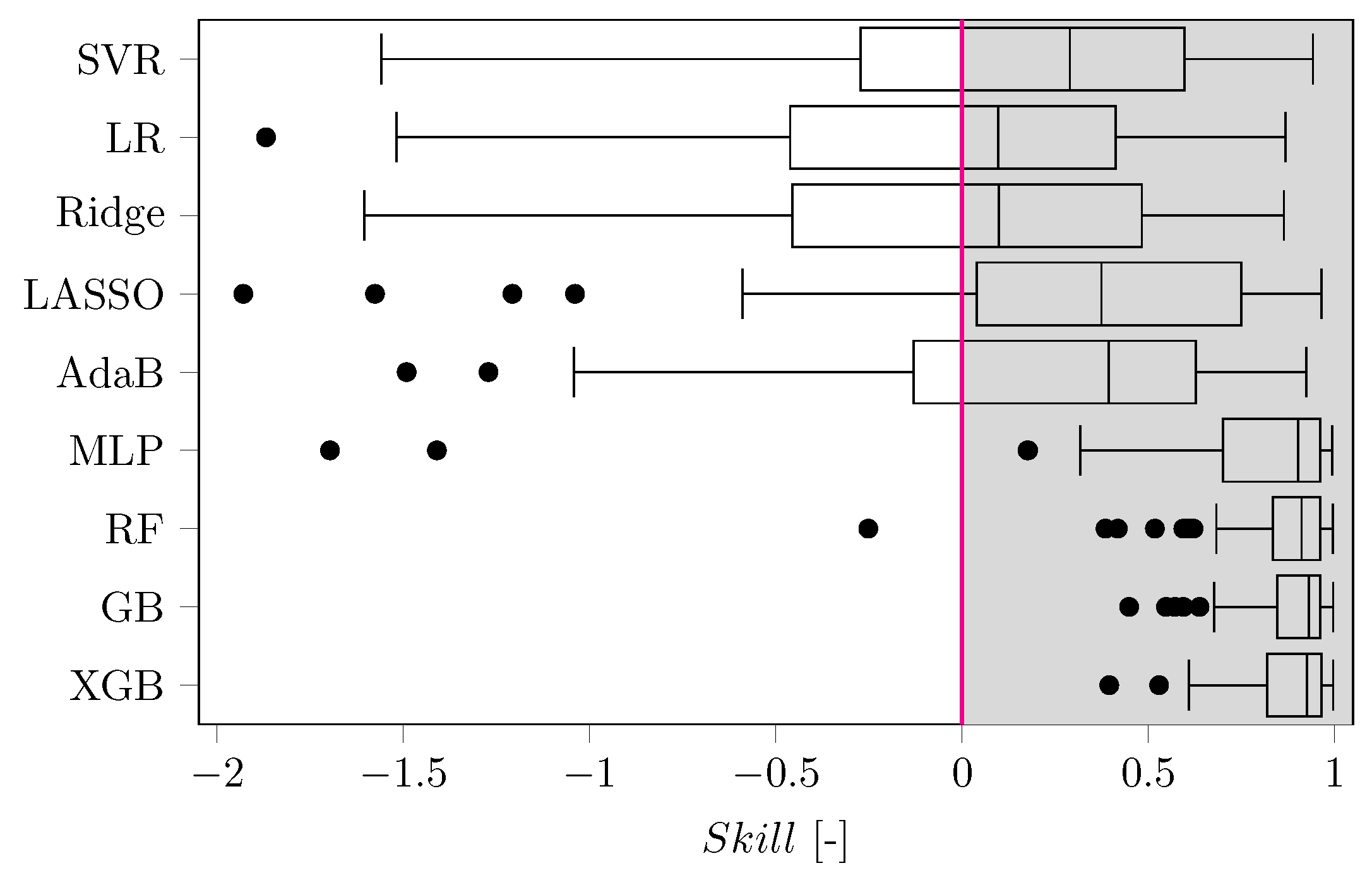
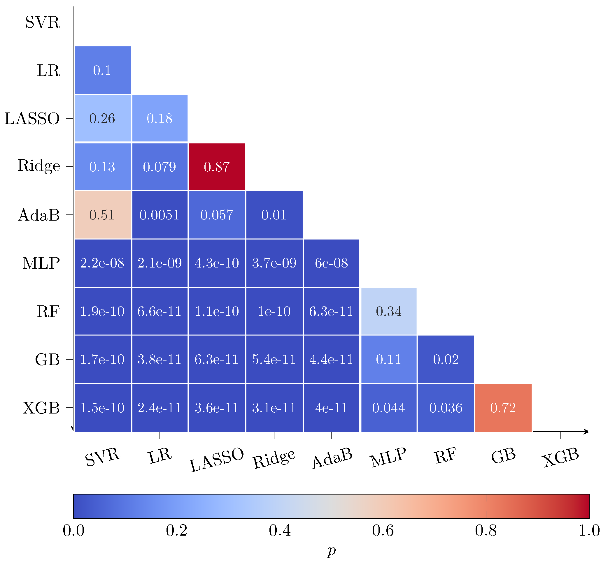
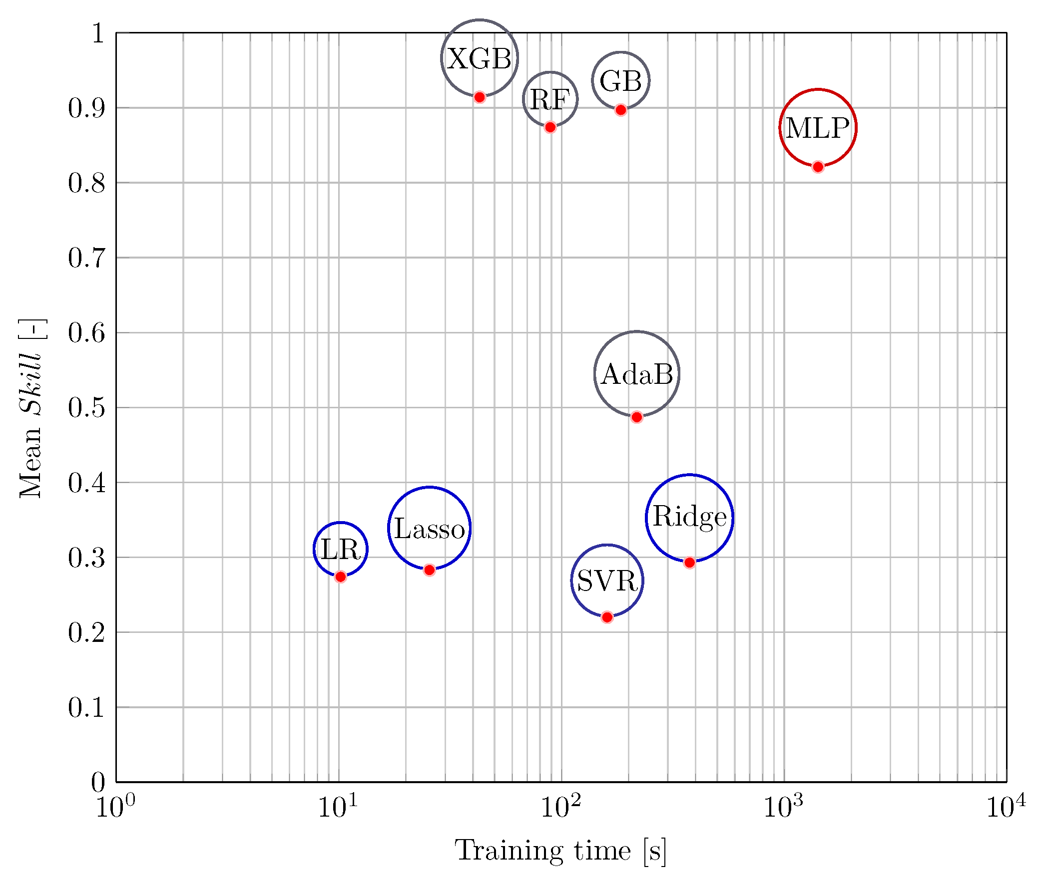
3.2. Comparison to ML Based Approaches

The results of the different models are summarized in Table 3. The regression performance is represented by the $Skill$ score.

In addition to the table, the results are visualized with the help of a boxplot per model class in Figure 8. It can be clearly seen that all ML methods are capable of predicting the flow stress of the AA7075 alloy with higher $Skill$ on average compared to the Z–A model.

As described in the previous sections, the LR model is the ML model with the lowest complexity. It is noticeable that Support Vector Regression (SVR), AdaBoost (AdaB), LASSO and Ridge Regression show a rather similar performance regarding $MSE$ and $Skill$. In contrast, the MLP shows a significantly higher mean $Skill$ with a reduced standard deviation. The average $Skill$ is increased further by the Random Forest model, but there are some poor performing outliers, directly indicated by the relatively high standard deviation. The Gradient Boosting (GB), as well as eXtreme Gradient Boosting (XGB), show the highest mean $Skill$ performance and the lowest variance between the results. Comparing the absolute values, it is noticeable that the mean $Skill$ of the XGB model is around 2% higher, while the standard deviations for both methods are nearly the same and the lowest of all investigated models. To support these findings, the Wilcoxon signed-rank test was performed. The $Skills$ of all model classes were tested for statistical significance and their p-values are compared in Figure 9. The p-value is a measure of the probability that an observed difference in the $Skill$ scores of the model could have occurred just by random chance. The lower the p-value, the more pronounced the statistical significance of the observed difference and vice versa. The $Skills$ of all models were tested against each other.

In Figure 9 it can be seen that the results of some ML model classes with inferior performance (SVR, LR, AdaB, LASSO, Ridge) do not significantly vary ($p>0.05$). The superior methods, i.e., GB and XGB, are not significantly different, but when compared to the other models, they are. In order to select a model for further investigations, the next step of the evaluation procedure takes the computation time into account, i.e., the time that each model class needed to run through an entire leave-one-out training loop. In Figure 10, the $Skill$ of the different model classes is shown over the computation time on a logarithmic scale.

As shown in Figure 10, the LR, Lasso and, Ridge models do not show a clear difference in their $Skills$. By regularization, LASSO and Ridge Regression are able to make small improvements in their prediction performance only at the cost of a higher computational effort. The MLP needs by far the highest computation time. For this comparison, it is important to mention that the training was conducted with the same hardware using a total of 16 cores. The MLP was trained on an Nvidia Tesla V100 GPU in addition to the existing CPUs. This further reveals that the three ensemble methods RF, GB and XGB show not only the highest performances but also a relatively low computational cost in the present work. In the previous step, the GB and the XGB model classes could be found to perform significantly better. By directly comparing the data displayed in Figure 10, it can be concluded that elevated temperature modeling of the AA7075 alloy using the XGB model can be performed 4.3 times faster compared to the GB method. For this reason, the results presented in the following sections consider the XGB model only.

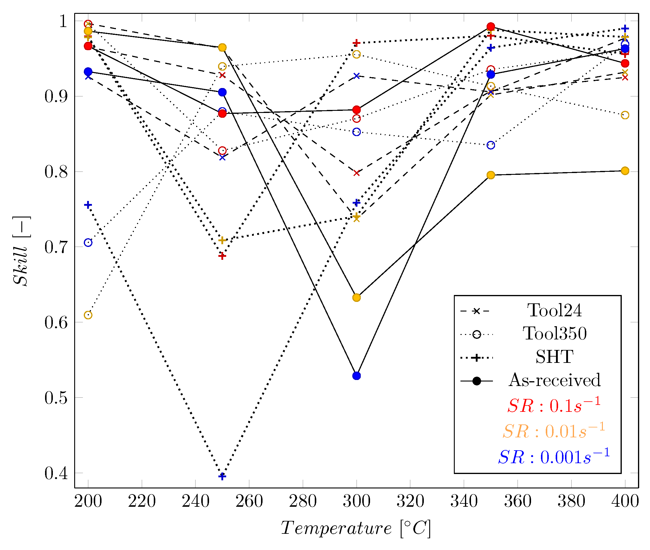
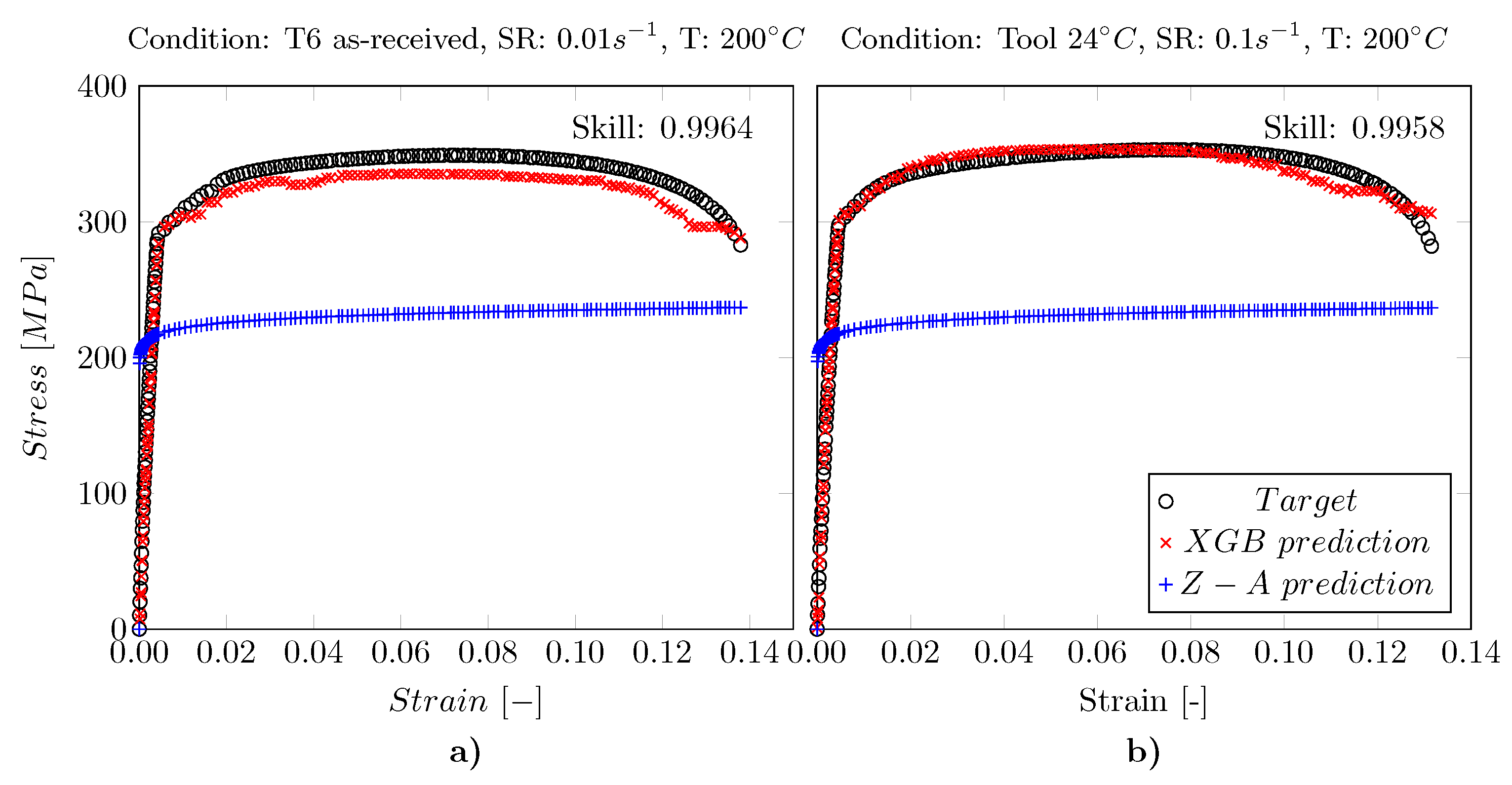
3.3. Results of the eXtreme Gradient Boosting

The 60 individual results of the evaluation using the XGB model are visualized in Figure 11.

Considering the results shown in Figure 11, it can be seen that there is no trend or pattern that allows deducing dependencies between the $Skill$ values and the conditions, temperature, or strain rate. In the case of the other model classes, no trend is recognizable (for brevity a detailed visualization for the other methods is omitted). The following Figure 12 shows an example of the two best predicted curves regarding the $Skill$ value compared with the prediction of the Z–A model. It can be seen that the experimental test data can be predicted with high $Skill$ using the XGB model. The $Skill$ values of the XGB are $0.9964$ for Figure 12a and $0.9958$ for Figure 12b.

The outliers of XGB in Figure 8 and Figure 11 respectively, demonstrate that also the XGB method is not capable of predicting all different curves with similar $Skill$ performance. For this reason, the two curves with the poorest $Skill$ values are shown in Figure 13. The $Skill$ values of the XGB are $0.5289$ for Figure 13a and $0.3952$ for Figure 13b. These $Skill$ values are rather low, however, they are still positive, meaning better than the Z–A reference model. It can be assumed, that the performance can be improved by using additional datasets of other temperatures, strain rates, or conditions allowing a more consistent prediction $Skill$ to be realized. Based on the error during training, the model is able to retrieve the training curves of the AA7075 alloy for all four considered conditions: T6, solution heat-treated, Tool $24{}^{\circ }$C, and Tool $350{}^{\circ }$C. Therefore, both the Z–A and the ML models considered in the present work can be further used for finite element analysis (FEA) applications as proposed by Li et al. in [3].

It is very important to note that, with the developed model, it is possible to make predictions for unknown parameter combinations based on the testing error. Other researchers and application engineers will be able to generate estimations for similar parameters, and in order to increase the generalization capability, even extend the existing model using data that are available for them. The results, material constants, and models obtained herein can be employed to simulate the true stress–strain curves at the deformation temperatures evaluated here. Eventually, the approaches and results shown will reduce the number of experiments needed for evaluating the forces required to be applied in the hot deformation of the alloy in focus. Such a reduction in the number of experiments will considerably save time and decrease costs.

As mentioned earlier, the occurrence of necking during tensile testing and softening mechanisms, i.e., DRV and DRX, render the modeling and prediction of material behavior difficult. However, attempts have been made to smooth the curves using a Savitzky–Golay filter [45]. This smoothing is based on higher degree linear regression in combination with a moving window. Due to the small number of samples per dataset, it is necessary to choose a very small window width in order to prevent excessive smoothing in the area of the transition from linear to non-linear flow behavior, in which case the smoothing in the posterior part of the curve is too weak. Obviously, a monotonically decreasing curve cannot be seen in all datasets. Therefore, smoothing of curves is beyond the scope of the present work and, hence, will be addressed in a follow-up study.

The results obtained in the present study are discussed with the literature in order to understand the accuracy of the models used. A strain-compensated Arrhenius model and an ANN model were found to be capable of predicting flow curves of AA7075 alloy obtained from compression experiments at elevated temperatures [25,46,47]. The error values reported are similar to the values calculated in the present study. However, due to the absence of necking during compression, the prediction of flow stress curves is less challenging compared to those obtained from tensile experiments. A modified J–C model was employed to predict the flow behavior of AA7075 alloy during tensile deformation at various temperatures and strain rates [48]. Although the modified J–C could generally predict the flow stress curves, disagreements between the experimental data and calculated points were considerable. Due to the difficulty of predicting the flow stress curves during tensile deformation, a physical plane-stress model was employed elsewhere to result in a lower level of mean average absolute relative error (AARE) [46]. The physical plane-stress model could slightly reduce the level of AARE compared to that of phenomenological ones. The present study reveals that the application of ML methods can also improve the accuracy of predicted flow stress curves, similar to the modified and physical-based models, and, hence, this modeling technique is suitable for the prediction of the tensile deformation behavior at elevated temperatures.

4. Conclusions

In the present work it was shown that it is possible to predict the flow stress behavior of aluminum alloy AA7075 at different temperatures and strain rates in tensile tests (in form of true stress–strain curves with low error) using ML methods taking different material conditions into account. It was also shown that the prediction of the flow stress using ML methods has a lower error compared to the classical Z–A approach. This could be due to the fact that the classical Z–A model could not reproduce the occurrence of necking at parameter combinations with low deformation temperatures. Even simple linear regression showed a lower mean $MSE$ compared to the conventional empirical model. The Random Forest, Gradient Boosting, and eXtreme Gradient Boosting models performed similarly well in terms of the $Skill$ score. The statistically significant difference in the $Skill$ scores of the models was confirmed using the Wilcoxon signed-rank test. XGB showed clear computational advantages compared to other high-performing models.

Many previous studies have been limited to MLPs, which have performed worse compared to the model classes assessed in the present work. The results obtained indicate that more complex models do not necessarily provide a higher performance, which should convince the community not to focus exclusively on MLPs but also to consider less complex models. A novelty in the work presented is the way of dividing the training and test data. The models were tested on entire curves with information learned from different, albeit related, curves. This approach allows for the use of large datasets and to generalize beyond available data. The presented data and models can be extended and improved with additional data, eventually allowing to save time and decrease the number of needed laboratory tests in the future. One possible extension to this is intelligent experimentation, where only those laboratory experiments that provide the most valuable information for the model are requested [49]. Another approach for improvement could be the use of Bayesian methods for modeling uncertainty. Such an approach could be promising due to the lack of big data being characteristic for the field of materials engineering.

References

1. Hirsch, J. Recent Development in Aluminium for Automotive Applications. Trans. Nonferrous Met. Soc. China 2014, 24, 1995–2002. [Google Scholar] [CrossRef]
2. Scharifi, E.; Sajadifar, S.V.; Moeini, G.; Weidig, U.; Böhm, S.; Niendorf, T.; Steinhoff, K. Dynamic Tensile Deformation of High Strength Aluminum Alloys Processed Following Novel Thermomechanical Treatment Strategies. Adv. Eng. Mater. 2020, 22, 2000193. [Google Scholar] [CrossRef]
3. Li, L.T.; Lin, Y.; Zhou, H.M.; Jiang, Y.Q. Modeling the High-Temperature Creep Behaviors of 7075 and 2124 Aluminum Alloys by Continuum Damage Mechanics Model. Comput. Mater. Sci. 2013, 73, 72–78. [Google Scholar] [CrossRef]
4. Senthil, K.; Iqbal, M.; Chandel, P.; Gupta, N. Study of the Constitutive Behavior of 7075-T651 Aluminum Alloy. Int. J. Impact Eng. 2017, 108, 171–190. [Google Scholar] [CrossRef]
5. Sajadifar, S.V.; Scharifi, E.; Weidig, U.; Steinhoff, K.; Niendorf, T. Performance of Thermo-Mechanically Processed AA7075 Alloy at Elevated Temperatures—From Microstructure to Mechanical Properties. Metals 2020, 10, 884. [Google Scholar] [CrossRef]
6. Lu, J.; Song, Y.; Hua, L.; Zheng, K.; Dai, D. Thermal Deformation Behavior and Processing Maps of 7075 Aluminum Alloy Sheet Based on Isothermal Uniaxial Tensile Tests. J. Alloys Compd. 2018, 767, 856–869. [Google Scholar] [CrossRef]
7. Lin, Y.C.; Li, L.T.; Fu, Y.X.; Jiang, Y.Q. Hot Compressive Deformation Behavior of 7075 Al Alloy under Elevated Temperature. J. Mater. Sci. 2012, 47, 1306–1318. [Google Scholar] [CrossRef]
8. Cerri, E.; Evangelista, E.; Forcellese, A.; McQueen, H. Comparative Hot Workability of 7012 and 7075 Alloys after Different Pretreatments. Mater. Sci. Eng. A 1995, 197, 181–198. [Google Scholar] [CrossRef]
9. McQueen, H.; Ryan, N. Constitutive Analysis in Hot Working. Mater. Sci. Eng. A 2002, 322, 43–63. [Google Scholar] [CrossRef]
10. Xiao, W.; Wang, B.; Wu, Y.; Yang, X. Constitutive Modeling of Flow Behavior and Microstructure Evolution of AA7075 in Hot Tensile Deformation. Mater. Sci. Eng. A 2018, 712, 704–713. [Google Scholar] [CrossRef]
11. Zhu, D.Y.; Zhen, L.; Lin, C.; Shao, W.Z. High Temperature Deformation Mechanism of 7075 Aluminum Alloy. Key Eng. Mater. 2007, 353–358, 691–694. [Google Scholar] [CrossRef]
12. Mirzaie, T.; Mirzadeh, H.; Cabrera, J.M. A Simple Zerilli–Armstrong Constitutive Equation for Modeling and Prediction of Hot Deformation Flow Stress of Steels. Mech. Mater. 2016, 94, 38–45. [Google Scholar] [CrossRef]
13. Zerilli, F.J. Dislocation Mechanics-Based Constitutive Equations. Metall. Mater. Trans. A 2004, 35, 2547–2555. [Google Scholar] [CrossRef]
14. Khan, A.S.; Liang, R. Behaviors of Three BCC Metal over a Wide Range of Strain Rates and Temperatures: Experiments and Modeling. Int. J. Plast. 1999, 15, 1089–1109. [Google Scholar] [CrossRef]
15. Zerilli, F.J.; Armstrong, R.W. Dislocation-mechanics-based Constitutive Relations for Material Dynamics Calculations. J. Appl. Phys. 1987, 61, 1816–1825. [Google Scholar] [CrossRef]
16. Sajadifar, S.; Yapici, G. High Temperature Flow Response Modeling of Ultra-Fine Grained Titanium. Metals 2015, 5, 1315–1327. [Google Scholar] [CrossRef]
17. Haghdadi, N.; Zarei-Hanzaki, A.; Khalesian, A.; Abedi, H. Artificial Neural Network Modeling to Predict the Hot Deformation Behavior of an A356 Aluminum Alloy. Mater. Des. 2013, 49, 386–391. [Google Scholar] [CrossRef]
18. Li, K.; Pan, Q.; Li, R.; Liu, S.; Huang, Z.; He, X. Constitutive Modeling of the Hot Deformation Behavior in 6082 Aluminum Alloy. J. Mater. Eng. Perform. 2019, 28, 981–994. [Google Scholar] [CrossRef]
19. Lin, Y.; Zhang, J.; Zhong, J. Application of Neural Networks to Predict the Elevated Temperature Flow Behavior of a Low Alloy Steel. Comput. Mater. Sci. 2008, 43, 752–758. [Google Scholar] [CrossRef]
20. Bahrami, A.; Mousavi Anijdan, S.; Ekrami, A. Prediction of Mechanical Properties of DP Steels Using Neural Network Model. J. Alloys Compd. 2005, 392, 177–182. [Google Scholar] [CrossRef]
21. Hodgson, P.; Kong, L.; Davies, C. The Prediction of the Hot Strength in Steels with an Integrated Phenomenological and Artificial Neural Network Model. J. Mater. Process. Technol. 1999, 87, 131–138. [Google Scholar] [CrossRef]
22. Song, S.H. A Comparison Study of Constitutive Equation, Neural Networks, and Support Vector Regression for Modeling Hot Deformation of 316L Stainless Steel. Materials 2020, 13, 3766. [Google Scholar] [CrossRef]
23. Li, B.; Pan, Q.; Yin, Z. Microstructural Evolution and Constitutive Relationship of Al–Zn–Mg Alloy Containing Small Amount of Sc and Zr during Hot Deformation Based on Arrhenius-Type and Artificial Neural Network Models. J. Alloys Compd. 2014, 584, 406–416. [Google Scholar] [CrossRef]
24. Sani, S.A.; Ebrahimi, G.; Vafaeenezhad, H.; Kiani-Rashid, A. Modeling of Hot Deformation Behavior and Prediction of Flow Stress in a Magnesium Alloy Using Constitutive Equation and Artificial Neural Network (ANN) Model. J. Magnes. Alloy. 2018, 6, 134–144. [Google Scholar] [CrossRef]
25. Quan, G.; Zou, Z.; Wang, T.; Liu, B.; Li, J. Modeling the Hot Deformation Behaviors of As-Extruded 7075 Aluminum Alloy by an Artificial Neural Network with Back-Propagation Algorithm. High Temp. Mater. Process. 2017, 36, 1–13. [Google Scholar] [CrossRef]
26. Sheikh-Ahmad, J.; Twomey, J. ANN Constitutive Model for High Strain-Rate Deformation of Al 7075-T6. J. Mater. Process. Technol. 2007, 186, 339–345. [Google Scholar] [CrossRef]
27. Desu, R.K.; Guntuku, S.C.; B, A.; Gupta, A.K. Support Vector Regression Based Flow Stress Prediction in Austenitic Stainless Steel 304. Procedia Mater. Sci. 2014, 6, 368–375. [Google Scholar] [CrossRef]
28. Song, S.H. Random Forest Approach in Modeling the Flow Stress of 304 Stainless Steel during Deformation at 700–900 °C. Materials 2021, 14, 1812. [Google Scholar] [CrossRef]
29. Sajadifar, S.V.; Scharifi, E.; Weidig, U.; Steinhoff, K.; Niendorf, T. Effect of Tool Temperature on Mechanical Properties and Microstructure of Thermo-Mechanically Processed AA6082 and AA7075 Aluminum Alloys. HTM J. Heat Treat. Mater. 2020, 75, 177–191. [Google Scholar] [CrossRef]
30. Scharifi, E.; Knoth, R.; Weidig, U. Thermo-Mechanical Forming Procedure of High Strength Aluminum Sheet with Improved Mechanical Properties and Process Efficiency. Procedia Manuf. 2019, 29, 481–489. [Google Scholar] [CrossRef]
31. Scharifi, E.; Savaci, U.; Kavaklioglu, Z.B.; Weidig, U.; Turan, S.; Steinhoff, K. Effect of Thermo-Mechanical Processing on Quench-Induced Precipitates Morphology and Mechanical Properties in High Strength AA7075 Aluminum Alloy. Mater. Charact. 2021, 174, 111026. [Google Scholar] [CrossRef]
32. Buitinck, L.; Louppe, G.; Blondel, M.; Pedregosa, F.; Mueller, A.; Grisel, O.; Niculae, V.; Prettenhofer, P.; Gramfort, A.; Grobler, J.; et al. API Design for Machine Learning Software: Experiences from the Scikit-Learn Project. arXiv 2013, arXiv:1309.0238. [Google Scholar]
33. Chen, T.; Guestrin, C. XGBoost: A Scalable Tree Boosting System. In Proceedings of the Proceedings of the 22nd ACM SIGKDD International Conference on Knowledge Discovery and Data Mining, San Francisco, CA, USA, 13–17 August 2016; ACM: San Francisco, CA, USA, 2016; pp. 785–794. [Google Scholar] [CrossRef]
34. Paszke, A.; Gross, S.; Massa, F.; Lerer, A.; Bradbury, J.; Chanan, G.; Killeen, T.; Lin, Z.; Gimelshein, N.; Antiga, L.; et al. PyTorch: An Imperative Style, High-Performance Deep Learning Library. arXiv 2019, arXiv:1912.01703. [Google Scholar]
35. Drucker, H.; Burges, C.J.C.; Kaufman, L.; Smola, A.; Vapnik, V. Support Vector Regression Machines. In Proceedings of the Advances in Neural Information Processing Systems, Denver, CO, USA, 2–5 December 1996; Mozer, M.C., Jordan, M., Petsche, T., Eds.; MIT Press: Cambridge, MA, USA, 1997; Volume 9, pp. 155–161. [Google Scholar]
36. Bottou, L.; Chapelle, O.; DeCoste, D.; Weston, J. Support Vector Machine Solvers. In Large-Scale Kernel Machines; MIT Press: Cambridge, MA, USA, 2007; pp. 1–27. [Google Scholar]
37. Basak, D.; Pal, S.; Patranabis, D. Support Vector Regression. Neural Inf. Process.-Lett. Rev. 2007, 11, 203–224. [Google Scholar]
38. Smola, A.J.; Schölkopf, B. A Tutorial on Support Vector Regression. Stat. Comput. 2004, 14, 199–222. [Google Scholar] [CrossRef]
39. Mendes-Moreira, J.; Soares, C.; Jorge, A.M.; Sousa, J.F.D. Ensemble Approaches for Regression: A Survey. ACM Comput. Surv. 2012, 45, 1–40. [Google Scholar] [CrossRef]
40. Dietterich, T.G. Ensemble Methods in Machine Learning. In Multiple Classifier Systems; Goos, G., Hartmanis, J., van Leeuwen, J., Eds.; Springer: Berlin/Heidelberg, Germany, 2000; Volume 1857, pp. 1–15. [Google Scholar] [CrossRef]
41. Nair, V.; Hinton, G.E. Rectified Linear Units Improve Restricted Boltzmann Machines. In Proceedings of the 27th International Conference on International Conference on Machine Learning, ICML’10, Haifa, Israel, 21–24 June 2010; Omnipress: Madison, WI, USA, 2010; pp. 807–814. [Google Scholar]
42. Clevert, D.A.; Unterthiner, T.; Hochreiter, S. Fast and Accurate Deep Network Learning by Exponential Linear Units (ELUs). arXiv 2016, arXiv:1511.07289. [Google Scholar]
43. Kingma, D.P.; Ba, J. Adam: A Method for Stochastic Optimization. arXiv 2017, arXiv:1412.6980. [Google Scholar]
44. Lin, Y.; Chen, X.M. A critical review of experimental results and constitutive descriptions for metals and alloys in hot working. Mater. Des. 2011, 32, 1733–1759. [Google Scholar] [CrossRef]
45. Savitzky, A.; Golay, M.J.E. Smoothing and Differentiation of Data by Simplified Least Squares Procedures. Anal. Chem. 1964, 36, 1627–1639. [Google Scholar] [CrossRef]
46. Yang, H.; Bu, H.; Li, M.; Lu, X. Prediction of Flow Stress of Annealed 7075 Al Alloy in Hot Deformation Using Strain-Compensated Arrhenius and Neural Network Models. Materials 2021, 14, 5986. [Google Scholar] [CrossRef] [PubMed]
47. Puchi-Cabrera, E.S.; Staia, M.H.; Ochoa-Pérez, E.; Barbera-Sosa, J.G.L.; Santana, Y.Y.; Villalobos-Gutiérrez, C.; Picón-Chaparro, J.R. Simple constitutive analysis of AA 7075-T6 aluminium alloy deformed at low deformation temperatures. Mater. Sci. Technol. 2012, 28, 668–679. [Google Scholar] [CrossRef]
48. Zhang, D.N.; Shangguan, Q.Q.; Xie, C.J.; Liu, F. A modified Johnson–Cook model of dynamic tensile behaviors for 7075-T6 aluminum alloy. J. Alloys Compd. 2015, 619, 186–194. [Google Scholar] [CrossRef]
49. Dingel, K.; Liehr, A.; Vogel, M.; Degener, S.; Meier, D.; Niendorf, T.; Ehresmann, A.; Sick, B. AI—Based On The Fly Design of Experiments in Physics and Engineering. In Proceedings of the 2021 IEEE International Conference on Autonomic Computing and Self-Organizing Systems Companion (ACSOS-C), Virtual Conference, 27 September–1 October 2021; pp. 150–153. [Google Scholar] [CrossRef]
Figure 1. (a) Roller hearth furnace and (b) forming tool used for sample production [5].
Crystals 12 01281 g001
Figure 2. Results of the tensile tests of the conditions: (a) T6 as-received, (b) Solutions heat-treated, (c) Tool 24 C and (d) Tool 350 C [5]. The color represents the temperature and the line style represents the strain rate respectively.
Crystals 12 01281 g002
Figure 3. Relationship between the logarithmic stress l n σ and the temperature T for the sample formed in the tool with a temperature of 350 C. The different lines are representing different strain values. For the sake of brevity and to provide a better overview, only 6 representative lines out of the originally 21 lines are shown.
Crystals 12 01281 g003
Figure 4. Relationship between l n σ and l n ϵ for the sample formed in the tool with a temperature of 350 C.
Crystals 12 01281 g004
Figure 5. Relationship between l n σ and l n ϵ ˙ at various strain values for the sample formed in the tool with a temperature of 350 C.
Crystals 12 01281 g005
Figure 6. Evaluation pipeline employed in the present study.
Crystals 12 01281 g006
Figure 7. Experimental data and Z–A modeling results depicting stress–strain curves of AA7075 samples formed in the tool with a temperature of 350 C for testing temperatures of (a) 200 C, (b) 250 C, (c) 300 C, (d) 350 C and (e) 400 C; Experimental data are shown by dashed lines, whereas, predicted data are highlighted by solid lines.
Crystals 12 01281 g007
Figure 8. Results of the predictions of the ML model classes visualized by boxplots. Evaluations with a higher S k i l l (or a lower M S E ) compared to the Z–A model are highlighted by the gray shaded area in the graph.
Crystals 12 01281 g008
Figure 9. p values as obtained from the Wilcoxon signed-rank test for the results of the investigated models.
Crystals 12 01281 g009
Figure 10. Comparison of the average test performances with respect to all 60 curves of the different models in relation to their required training time. The color represents the defined model categories. See text for details.
Crystals 12 01281 g010
Figure 11. All 60 test S k i l l values obtained for the XGB model, shown in relation to temperature. The color represents the strain-rate (SR), the marker and line style are representing the condition.
Crystals 12 01281 g011
Figure 12. The two curves being characterized by the highest test performance when applying the XGB model as directly compared to predictions made by the Z–A model. Subfigure (a) shows the T6 as-received condition at a strain rate of 0.01 s 1 at 200 C whereas in (b) the Tool 24 C condition at a strain rate of 0.1 s 1 at a temperature of 200 C can be seen.
Crystals 12 01281 g012
Figure 13. The two curves with the lowest test performance when applying the XGB model compared with model predictions of the Z–A model. Subfigure (a) shows the Tool 350 C condition at a strain rate of 0.001 s 1 at 300 C whereas in (b) the Solution heat-treated (SHT) condition at a strain rate of 0.001 s 1 at a temperature of 250 C can be seen.
Crystals 12 01281 g013