Transformation of 2D RVE Local Stress and Strain Distributions to 3D Observations in Full Phase Crystal Plasticity Simulations of Dual-Phase Steels

Abstract

Crystal plasticity-based numerical simulations help understand the local deformation behavior of multiphase materials. It is known that in full phase simulations, the local 2-dimensional (2D) representative volume elements (RVEs) results are distinctly different from 3-dimensional (3D) RVEs. In this work, the difference in the results of 2D and 3D RVEs is investigated systematically, and the effect of magnification, total strain and composition are analyzed. The 3D RVEs of dual-phase (DP)-steel are generated using DREAM-3D. The 2D RVEs are the sliced surfaces of corresponding 3D RVEs for a direct pixel-to-pixel comparison of results. It is shown that the corresponding 3D distribution can be rapidly derived from the 2D result based on the alternative error and least square method. The interactive parameters for these processes are identified and analyzed for the ferrite phase, which provides information about the convergence. Examined by qualitative and quantitative statistical analysis, it is shown that the corresponding 2D distribution by the fourth iteration has a prominent similarity with the exact 3D distribution. The work presented here contributes toward solving the paradox of comparing local strain from 2D crystal plasticity (CP) simulations with the effective 3D specimen used for tests.

1. Introduction

Multiple-phase composites possess admirable mechanical properties and service life. Combining softer matrix with harder islands [1], multiple-phase materials demonstrate the strong structure and ductility, such as in dual-phase steel (DP steel) [2], metal matrix composites, and other advanced steel [3]. The material properties of the multiphase materials depend on the microstructural attributes, such as the size, shape, composition, and distribution of the second phase within the matrix [4]. The effect of these attributes is interdependent and plays a key role in defining the deformation and damage behavior under varying loading conditions [5,6], i.e., strain rate, temperature, and loading direction. Numerical simulation models provide an interesting outlook for targeted material development by avoiding the expensive and time-consuming experimentation of every iterative modification in the material microstructure [7,8,9].

There are different numerical simulation models, i.e., empirical, analytical, data-driven, and hybrid [10,11]. Although they are useful in the general modeling of material deformation and damage behavior, they lack the fundamental dependence on the local microstructural attributes [12,13]. Fast Fourier transformation-based crystal plasticity models provide a comprehensive and accurate solution for modeling the multiphase material’s dependence on the microstructural attributes [14,15]. The RVEs in such models comprise all the necessary phase compositions, size, orientation, and distribution that represent the actual material [16]. Therefore, the model’s accuracy and applicability largely depend on the constructed RVE for such simulations.

Different simple and sophisticated models for accurate RVE development have been proposed previously, i.e., single-step Voronoi tessellation, multi-step Voronoi tessellation, and artificial neural networks yielding accurate results that are usually 3D. According to the RVE [17] method, both 2D (2-dimension) [18] and 3D (3-dimension) [19] microstructures have been constructed by random grain size, orientation, phase, and texture or measured from electron backscatter diffraction (EBSD) data [20]. Based on EBSD patterns from the serial-sectioning experiments, 3D polycrystalline microstructures were constructed by Groeber et al. [21,22]. Recently, DREAM-3D [23] was used to construct realistic RVEs from virtual or real statistical grain size, orientation, and texture data. Applying DREAM-3D and DAMASK [24], the performance of multilayer composites can be evaluated under mechanical loading by the crystal plasticity material model.

Compared to the simulation and experimental data for DP steels, Ramazani et al. [25] discovered that the 2D model displayed underestimated behavior, while the 3D result demonstrated a quantitative description of the flow curve in comparison to the experimental data. Qayyum et al. [26,27] studied the local deformation and transformation behavior of transformation-induced plasticity (TRIP) steel. In these articles, the simulation results of global stress and strain behavior were compared to the experimental result. Nevertheless, the validation of local distribution in 3D has a challenge to discuss, owing to the inconsistency between experiment and simulation results. Diehl et al. [28] analyzed the effect of “columnarity” and studied the influence of the nearby environment on stress and strain in DP microstructures. It was discovered that the local stress and strain distributions are strongly influenced by both the nearby grain shape and grain orientation. Due to this effect, the 2D simulations of heterogeneous microstructures could be definitely misleading for the damage prediction [29] of crack initiation and propagation.

The CP models are also largely dependent on several physical and a few fitting parameters. These parameters are obtained by comparing averaged numerical simulation results with experimental stress and strain curves [26,30]. Although a certain set of fitted parameters seems to accurately represent the overall deformation behavior, a slightly different set of fitted parameters is also expected to yield similar global results with a significant change in local results. This reliability of such models on the globally calibrated parameters can lead to incorrect local results. In the recent past, researchers have developed algorithms for automated sensitivity analyses and parametric identifications from global stress and strain curves [31,32]. A more reliable way of calibrating and validating the CP model parameters can be through direct local comparison of experimental in situ and simulation results.

The local strain measurement is experimentally possible now due to the advancement of in situ measurement and data processing tools, which can accurately capture local strain distribution and local microstructural attributes [33,34,35]. However, constructing an accurate 3D RVE of the same specimen is a paradox as 3D EBSD requires polishing, slicing, and measurement throughout the specimen. Moreover, different phases frequently cause false detection at the measurement surfaces and the grain boundaries [36].

Therefore, to carry out such a comparison, the 2D RVE results from CP simulation should be reliably transformed to keep the global results the same while transforming the local stress and strain distributions for comparison with the results of the 3D material surface. It is a mathematical challenge that can yield a model for transforming 2D RVE simulation results of local strain distribution for comparison with strain measurements on the surface of a 3D specimen. Recently, Qayyum et al. [37,38] investigated the stress and strain distribution between 2D and 3D RVEs with different total grain numbers. It was shown that the global distribution of the flow curve is similar across different RVEs. However, the local distribution showed obvious variation. The numerical finding of Qayyum et al. [37,38] underlines the different stress and strain distribution in 2D and 3D via random distribution of grain size and orientation. In the current article, the previous study is carried one step further, and a corresponding local 3D stress and strain distribution on the RVE surface is achieved by transforming 2D stress and strain. The work is based on the alternative error and least square method. The transformation of the ferrite phase stress and strain from the 2D result is iteratively achieved. The iterative constants for different cases of magnification, strain levels, and volume fractions are presented and compared. The proposed new numerical approach is helpful in iteratively transforming the 2D stress and strain if the 3D outcome is known. To analyze and compare the derived 3D distribution with actual results, a statistical analysis of the obtained data is carried out.

The following Section 2 presents the detail of the numerical simulation model, including grain size, boundary condition, and material parameter of crystal plasticity. Then, the proposed iterative method, which is adopted in the current work, is explained in Section 3. Next, the derived 3D local stress and strain distribution calculated using the proposed method are displayed. Meanwhile, similarities between derived and exact 3D distribution are provided by statistical analysis in Section 4. Finally, the discussion and conclusion are presented in Section 5 and Section 6.

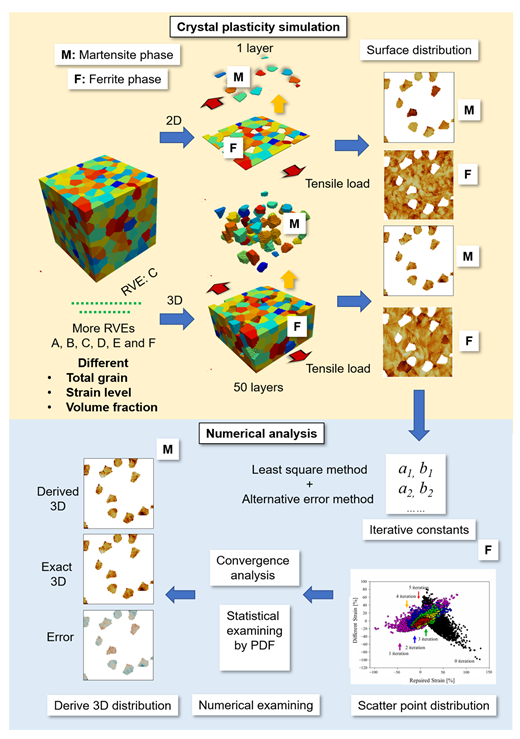
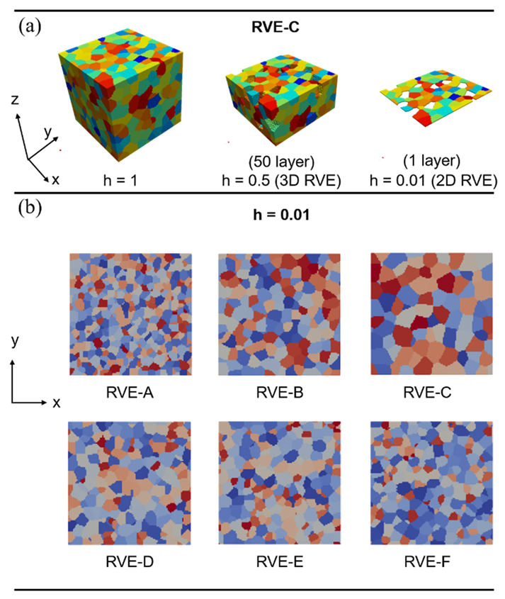
2. Numerical Simulation Model

The material adopted in the current investigation is DP steel, which comprises two distinct phases, i.e., soft ferrite matrix and hard martensite island. This large local microstructural heterogeneity yields significant local strain contrast during deformation. The microstructural distribution, grain size, material properties, and grain orientation are adopted from previously published work [39,40,41]. This article investigates different parameters for varying the overall number of grains, strain levels, and volume fractions.

Table 1. Grain size distribution, number of total grain, volume fraction, and strain level for the microstructure [37].

Case	RVE	Ferrite Grains			Martensite Grains			Total Grain	Strain Level [%]	Volume Fraction
		Min.	Max.	Avg.	Min.	Max.	Avg.
1	A	5.1	7.6	6.35	3.5	5.7	4.6	8400	25	0.1
2	B	8.5	12.7	10.6	5.4	8.8	7.1	1900	25	0.1
3	C	11.2	16.8	14.0	9.8	15.8	12.8	700	25	0.1
4	D	8.5	12.7	10.6	5.4	8.8	7.1	1900	5	0.1
5	D	8.5	12.7	10.6	5.4	8.8	7.1	1900	15	0.1
6	D	8.5	12.7	10.6	5.4	8.8	7.1	1900	25	0.1
7	D	8.5	12.7	10.6	5.4	8.8	7.1	1900	15	0.1
8	E	8.5	12.7	10.6	5.4	8.8	7.1	1900	15	0.15
9	F	8.5	12.7	10.6	5.4	8.8	7.1	1900	15	0.2

demonstrates the grain size distribution of ferrite and martensite, number of total grains, volume fractions, and strain levels for each model. For cases 1 to 3, the varying parameter is the total number of grains; for cases 4 to 6, the varying parameter is strain level; For cases 7 to 9, the varying parameter is volume fraction. Note that the unit of grains size is µm and total grain is a dimensionless value. Based on experimental observation [42], the smaller average grain sizes of ferrite and martensite were assigned as 6.35 and 4.6 in RVE-A, whereas the larger average grain sizes were 14.0 and 12.8 in RVE-C during the crystal plasticity simulation. Hence, the total grains of RVE-A are more than RVE-C.

A cubic equiaxed crystal structure and ellipsoid grain shape are assigned to both ferrite and martensite phases. 100 × 100 × 100 voxels RVEs are systematically constructed using DREAM-3D for the sizes as shown in Table 1. Figure 1 shows a schematic diagram and flow chart in this article. The blue arrows indicate the steps involved in carrying out this work. In the beginning, 2D and 3D simulations for different RVEs are carried out. Both ferrite (F) and martensite (M) phases are then individually analyzed. Combined with the least square and alternative error method, the iterative constants ($a_1$, $b_1$, $a_2$, and $b_2$, …) of the linear equation are calculated while transforming the 2D results into 3D.

The principal aim of this ongoing study is to develop a robust methodology for deriving the 3D surface stress and strain distribution from the 2D RVE result for ferrite and martensite phases. This work brings us one step closer to that aim. As a representation, RVE-C in inverse pole figure (IPF) colors is shown in Figure 2a (h = 1), where h indicates the length of z-direction normalized total length of z-direction. Following Qayyum et al. [37], 50- (h = 0.5) and 1-layer (h = 0.01) RVE were sliced from the initial microstructure and regarded as 3D and 2D RVE, respectively. The simulation results for 1- and 50-layers have been selected and defined as 2D and 3D results of the local stress and strain distribution. There are 10,000 Gaussian mesh elements in one layer, meaning 2D and 3D possess 10,000 and 500,000 elements, respectively. All the constructed RVEs were sliced into similar geometries with 1-layer (h = 0.01) RVE and shown in terms of texture style in Figure 2b.

The ferrite and martensite are defined as elastic–viscoplastic deformable phases. The elastic stiffness, shear resistance, hardening behavior, and curve fitting parameter are adapted from previously published work [38] and presented in

Table 2. Mechanical properties of multiphase (ferrite and martensite) were adopted from [37] for simulation modeling.

Parameter	Symbol	Ferrite	Martensite	Unit
First elastic stiffness constant with normal strain	C11	233.3	417.4	GPa
Second elastic stiffness constant with normal strain	C12	135.5	242.4	GPa
First elastic stiffness constant with shear strain	C44	128.0	211.1	GPa
Initial shear resistance on [111]	S0 [111]	95	406	MPa
Saturation shear resistance on [111]	S∞ [111]	222	873	MPa
Initial shear resistance on [112]	S0 [112]	96	457	MPa
Saturation shear resistance on [112]	S∞ [112]	412	971	MPa
Slip hardening parameter	h0	1.0	563	GPa
Interaction hardening parameter	hα,β	1.0	1.0	-
Stress exponent	$n$	20	20	-
Curve fitting parameter	$w$	2.0	2.0	-

.

The crystallographic orientation, mechanical properties, and phase of ferrite and martensite are included in the RVE geometry definition. A uniaxial load along the x-direction is defined using mixed boundary conditions as follows:

$${\dot{\mathit{F}}}_{ij}=\left[\begin{array}{ccc}1& 0& 0\\ 0& *& 0\\ 0& 0& *\end{array}\right]\times {10}^{-3}·s^{-1}$$

(1)

$${\mathit{P}}_{ij}=\left[\begin{array}{ccc}*& *& *\\ *& 0& *\\ *& *& 0\end{array}\right]Pa$$

(2)

where ${\dot{\mathit{F}}}_{ij}$ is the coefficients of the macroscopic rate of the deformation gradient, ${\mathit{P}}_{ij}$ is the first Piola–Kirchhoff stress. ${\dot{F}}_{11}=1/s$ indicates tensile condition, 0 is represented as restricted, and * is an arbitrary value during the simulation. It should be noted that the strain rate of all simulations is assumed to be $1\times {10}^{-3}/s$ in conjunction with periodic boundary conditions in all three directions. The simulations are performed in plain strain mode, where 2D RVE is interpreted as a columnar grain structure.

The spectral method via fast Fourier transform [43] is used to solve the continuum mechanics formulation mentioned above. After completing simulations, the 2D and 3D data are statistically analyzed. The 3D numerical results are used as a reference for iteratively modifying the 2D results by combining the least square and alternative error methods via Matlab programs (2019b, The MathWorks Inc., Natick, MA, USA).

3. Method

In the beginning, both the 50- and 1-layers were regarded as geometry models for crystal simulation and considered as 3D and 2D RVE models, as shown in Figure 2a. Note that stress/strain throughout this article means either stress or strain conditions. The results from the 2D RVE are compared with the surface of the corresponding 3D RVE to analyze the difference in stress/strain values. First, the stress/strain on the 2D layer result with respect to the difference in stress/strain between the 3D and 2D layer results is considered. Based on the least square method, the linear equation for this can be written as follows:

$$y_{1\mathrm{i}}=a_1{x}_{1\mathrm{i}}+b_1, \hspace{1em}\hspace{1em}\mathrm{i}=1,2,3\dots \dots 10,000$$

(3)

$$a_1=\frac{{\displaystyle {\sum }_{\mathrm{i}=1}^{10,000}(f_{1\mathrm{i}}-\overline{f_1})(f_{\mathrm{er}0\mathrm{i}}-\overline{f_{\mathrm{er}0}})}}{{\displaystyle {\sum }_{\mathrm{i}=1}^{10,000}{(f_{1\mathrm{i}}-\overline{f_1})}^2}}, b_1=\overline{f_{\mathrm{er}0}}-a_1\overline{f_1}, \mathrm{i}=1,2,3\dots \dots 10,000$$

(4)

where $\mathrm{i}$ is the number of elements on the top surface, and there are 100 × 100 voxels on both 2D and 3D layers. Where $f_{1\mathrm{i}}$ is stress/strain for 2D layer result; $\overline{f_1}$ is average stress/strain for 2D layer result; $f_{50\mathrm{i}}$ is stress/strain for 3D layer result; $f_{\mathrm{er}0\mathrm{i}}$ is the difference in stress/strain between 3D and 2D layer results ($f_{\mathrm{er}0\mathrm{i}}=f_{50\mathrm{i}}-f_{1\mathrm{i}}$), which indicates the difference of non-revised (original 2D) stress/strain; and $\overline{f_{\mathrm{er}0}}$ is the average difference in stress/strain between 3D and 2D layer results.

Through this method, the corresponding $y_{1\mathrm{i}}$, $a_1$, and $b_1$ can be obtained. Hence, the first revised stress/strain ($f_{\mathrm{r}1\mathrm{i}}$) and the different first revised stress/strain ($f_{\mathrm{er}1\mathrm{i}}$) can be derived:

$$f_{\mathrm{r}1\mathrm{i}}=f_{1\mathrm{i}}+y_{1\mathrm{i}}, \mathrm{i}=1,2,3\dots \dots 10,000$$

(5)

$$f_{\mathrm{er}1\mathrm{i}}=f_{50\mathrm{i}}-f_{\mathrm{r}1\mathrm{i}}, \mathrm{i}=1,2,3\dots \dots 10,000$$

(6)

where $f_{\mathrm{er}1\mathrm{i}}$ can be calculated by the difference in stress/strain between the 3D layer and the first revised 2D layer result. However, if the error of the first revision is not convergent, the second iteration will be carried out.

Next, the difference in stress/strain between the 3D and 2D layer results is considered with respect to the different first revised stress/strain. Based on the least square method, the linear equation can be obtained as follows:

$$y_{2\mathrm{i}}=a_2{x}_{2\mathrm{i}}+b_2, \mathrm{i}=1,2,3\dots \dots 10,000$$

(7)

$$a_2=\frac{{\displaystyle {\sum }_{\mathrm{i}=1}^{10,000}(f_{\mathrm{er}0\mathrm{i}}-\overline{f_{\mathrm{er}0}})(f_{\mathrm{er}1\mathrm{i}}-\overline{f_{\mathrm{er}1}})}}{{\displaystyle {\sum }_{\mathrm{i}=1}^{10,000}{(f_{\mathrm{er}0\mathrm{i}}-\overline{f_{\mathrm{er}0}})}^2}},b_2=\overline{f_{\mathrm{er}1}}-a_2\overline{f_{\mathrm{er}0}}, \mathrm{i}=1,2,3\dots \dots 10,000$$

(8)

Through this method, the corresponding $y_{2i}$ and $x_{2i}$ can be obtained. Hence, the second revised stress/strain ($f_{\mathrm{r}2\mathrm{i}}$) and the different second revised stress/strain ($f_{\mathrm{er}2\mathrm{i}}$) can be derived:

$$f_{\mathrm{r}2\mathrm{i}}=f_{\mathrm{r}1\mathrm{i}}+y_{2\mathrm{i}}, \mathrm{i}=1,2,3\dots \dots 10,000$$

(9)

$$f_{\mathrm{er}2\mathrm{i}}=f_{50\mathrm{i}}-f_{\mathrm{r}2\mathrm{i}}, \mathrm{i}=1,2,3\dots \dots 10,000$$

(10)

$f_{\mathrm{er}2\mathrm{i}}$ can be calculated by the difference in stress/strain between the 3D layer and the second revised stress/strain. Finally, based on the least square method, a general linear equation can be obtained in the series form of m-iteration. The difference in the m-2 revised stress/strain (x-axis) is considered with respect to the different m-1 (y-axis) revised stress/strain. This equation can be written as follows:

$$y_{\mathrm{mi}}=a_{\mathrm{m}}{x}_{\mathrm{mi}}+b_{\mathrm{m}}, \mathrm{i}=1,2,3\dots \dots 10,000,\mathrm{m}=2,3,4,\dots$$

(11)

$$\begin{gathered} a_{\mathrm{m}}=\frac{{\displaystyle {\sum }_{\mathrm{i}=1}^{10,000}(f_{\mathrm{er}(\mathrm{m}-2)\mathrm{i}}-\overline{f_{\mathrm{er}(\mathrm{m}-2)}})(f_{\mathrm{er}(\mathrm{m}-1)}-\overline{f_{\mathrm{er}(\mathrm{m}-1)}})}}{{\displaystyle {\sum }_{\mathrm{i}=1}^{10,000}{(f_{\mathrm{er}(\mathrm{m}-2)\mathrm{i}}-\overline{f_{\mathrm{er}(\mathrm{m}-2)}})}^2}}, b_{\mathrm{m}}=\overline{f_{\mathrm{er}(\mathrm{m}-1)}}-a_{\mathrm{m}}\overline{f_{\mathrm{er}(\mathrm{m}-2)}}, \\ \mathrm{i}=1,2,3\dots \dots 10,000,\mathrm{m}=2,3,4,\dots \end{gathered}$$

(12)

Through this method, the corresponding $y_{\mathrm{mi}}$ and $x_{\mathrm{mi}}$ can be obtained. Hence, the m revised stress/strain ($f_{\mathrm{rmi}}$) and the different m revised stress/strain ($f_{\mathrm{ermi}}$) can be derived as:

$$f_{\mathrm{rmi}}=f_{\mathrm{r}(\mathrm{m}-1)\mathrm{i}}+y_{\mathrm{mi}}, \mathrm{i}=1,2,3\dots \dots 10,000, \mathrm{m}=2,3,4,\dots$$

(13)

$$f_{\mathrm{ermi}}=f_{50\mathrm{i}}-f_{\mathrm{rmi}}, \mathrm{i}=1,2,3\dots \dots 10,000, \mathrm{m}=2,3,4,\dots$$

(14)

$f_{\mathrm{ermi}}$ can be calculated by the difference in stress/strain between the 3D layer and the m revised stress/strain.

4. Results

Although results for both the ferrite and martensite phase were processed and analyzed in this work, in this section, the results for the ferrite phase are presented. Similar numerical results (

Table A1. Constants $a_m$, $b_m$, and $R_m^2$ (m = 1, 2, 3, 4) for the martensite phase of linear equation with stress condition by the proposed iterative method.

Stress
Analysis Parameter	Total Grain			Strain Level			Volume Fraction
	8400	1900	770	5%	15%	25%	0.1	0.15	0.2
Case	1	2	3	4	5	6	7	8	9
RVE Iterative Const.	A	B	C	D	D	D	D	E	F
$a_1$	−0.86	−0.78	−0.88	−0.7375	−0.7938	−0.82	−0.7938	−0.725	−0.766
$b_1$	1875	1614	1746	1526	2002	2222	2002	2092	1956
$R_1^2$	0.31	0.23	0.36	0.14	0.24	0.34	0.24	0.21	0.17
$a_2$	0.67	0.76	0.63	0.84	0.74	0.64	0.74	0.77	0.81
$b_2$	6.02	2.87	−1.003	28.96	14.86	6.64	14.86	20.6	−25.19
$R_2^2$	0.67	0.76	0.63	0.84	0.74	0.64	0.74	0.79	0.81
$a_3$	0.32	0.23	0.36	0.15	0.25	0.35	0.25	0.23	0.18
$b_3$	4.67	1.05	−1.00	5.69	6.49	6.37	6.49	6.55	−5.52
$R_3^2$	0.31	0.23	0.36	0.14	0.25	0.35	0.25	0.23	0.17
$a_4$	0.68	0.76	0.63	0.86	0.75	0.65	0.75	0.77	0.82
$b_4$	5.68	1.35	−1.00	8.39	8.43	7.14	8.43	6.24	−6.69
$R_4^2$	0.68	0.76	0.63	0.86	0.75	0.65	0.75	0.77	0.82

and

Table A2. Constants $a_m$, $b_m$, and $R_m^2$ (m = 1, 2, 3, 4) for the martensite phase of linear equation with strain condition by the proposed iterative method.

Strain
Analysis Parameter	Total Grain			Strain Level			Volume Fraction
	8400	1900	770	5%	15%	25%	0.1	0.15	0.2
Case	1	2	3	4	5	6	7	8	9
RVE Iterative Const.	A	B	C	D	D	D	D	E	F
$a_1$	−0.31	0.09	0.5354	0.26	0.23	0.18	0.23	0.22	−0.03
$b_1$	2.19	−0.023	−1.3028	−0.30	−0.93	−1.38	-0.93	−0.3	0.60
$R_1^2$	0.005	0.0007	0.015	0.003	0.002	0.002	0.002	0.006	0.001
$a_2$	0.99	0.99	0.98	0.99	0.99	0.99	0.99	0.99	0.99
$b_2$	0.17	−0.12	−0.4026	0.028	0.104	0.16	0.104	−0.32	−0.53
$R_2^2$	0.99	0.99	0.98	0.99	0.99	0.99	0.99	0.99	0.99
$a_3$	0.005	0.0008	0.0164	0.003	0.003	0.002	0.003	0.006	0.001
$b_3$	0.0009	−0.00008	−0.0058	0	0	0	0	0	0
$R_3^2$	0.005	0.0007	0.0156	0.003	0.003	0.002	0.003	0.006	0.001
$a_4$	0.99	0.99	0.9850	0.996	0.997	0.998	0.997	0.993	0.99
$b_4$	0.001	−0.00015	−0.0091	0	0	0	0	0	0
$R_4^2$	0.99	0.99	0.98	0.996	0.997	0.998	0.998	0.993	0.99

) of the martensite phase are provided in Appendix A of this article for interested readers.

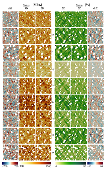
4.1. Local Stress/Strain Distribution in 2D and 3D

Initially, local stress/strain distributions for case 1 to case 9 are shown in Figure 3 to address how the local results vary between 2D and 3D separately sourced from 1- and 50-layers only for ferrite matrix. Note that case 1 to case 3 indicates different total grain numbers; case 4 to case 6 indicate different strain levels; case 7 to case 9 indicates different volume fractions. The detailed microstructure information is demonstrated in Table 1. To point out the difference between 2D and 3D-RVEs, the local stress and strains are arithmetically subtracted (3D−2D) as $f_{er0i}=f_{50i}-f_{1i}$, and the difference map with the true stress or strain scales −700 to 700 MPa −60 to 60%, respectively, is shown in Figure 3.

For 2D conditions, high contrast in the stress/strain concentration is observed. It can be noted that there is a significant difference between the 3D and 2D-RVEs local attribute distribution. In the 3D RVE case, the stress and strain are relatively homogeneously distributed and display lower contrast. Meanwhile, the higher stress/strain transfer to the martensite/ferrite interface. It can be concluded that the local stress/strain distribution is different from 3D and 2D-RVEs, regardless of the total grain numbers, strain levels, and volume fractions. Therefore, a straightforward transformation method can hardly be adapted to modify 2D results to 3D distribution for a specific element. The results from the proposed numerical statistical analysis are given in the next section.

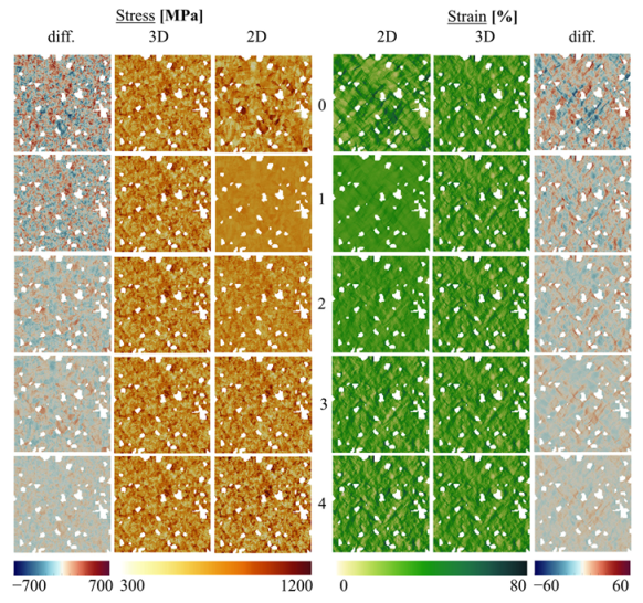
4.2. Step by Step for Transformation from 2D to 3D

In Section 2, the proposed iterative method was derived for this specific problem. Figure 4 shows a scatter diagram of the ferrite phase with two extreme “total grain number” cases (case 1 (a, c) and case 3 (b, d)) via different iterative steps both for stress (a, b) and strain (c, d) value. Since all the cases are similar, this article only presents cases 1 and case 3 for discussion. Regarding the x-axis, the repaired stress/stain is indicative of the corresponding different revised stress/strain of 2D. It assumes 2D stress/strain ($f_{1i}$) for the zero iteration, but for the first iteration and onwards, it is derived to $f_{\mathrm{er}0\mathrm{i}}$ and Equation (6) for the first and second iteration, respectively. For the y-axis, the different stress/strain comes from the general form in Equation (14), where the 2D revised stress/strain compared with 3D stress/strain is computed for each solution point. This term is now clearly used and mentioned in the explanation of $f_{\mathrm{er}0\mathrm{i}}$ for the zero iteration. Then, Equations (6) and (10) indicate the first and second iteration, respectively.

For the same iterative step, the numerical distribution reveals a similar tendency regardless of different total grain numbers for stress cases, as shown in Figure 4a,b, or for strain cases, as shown in Figure 4c,d, respectively. For the initial condition, the stress/strain on the 2D layer result ($f_{1i}$) with respect to the difference of non-revised stress/strain between 2D and 3D layer results ($f_{er0i}$) are defined as black scatter, as shown in Figure 4. It can be observed that the stress/strain results in 2D have inverse behavior to the difference in stress/strain between the 3D and 2D layer results. Due to inverse behavior, it can be speculated that the larger value of stress/strain is overestimated, and the lower value of stress/strain is underestimated for the 2D layer result. Transferring the local stress/strain of a 2D layer to match the 3D layer better, a larger value of stress/strain should be forcibly applied to a negative value of stress/strain, and a positive value of stress/strain should be forcibly applied to a smaller one.

Based on the least square method, the linear equation for the original condition can be calculated in Equations (3) and (4).

Table 3. Constants $a_m$, $b_m$, and $R_m^2$ (m = 1, 2, 3, 4) for the ferrite phase of linear equation with stress condition by the proposed iterative method.

Stress
Analysis Parameter	Total Grain			Stress/Strain Level, %			Volume Fraction, %
	8400	1900	770	5	15	25	0.1	0.15	0.2
Case	1	2	3	4	5	6	7	8	9
RVE Iterative Const.	A	B	C	D	D	D	D	E	F
$a_1$	−0.76	−0.81	−0.75	−0.63	−0.74	−0.78	−0.74	−0.66	−0.66
$b_1$	543.73	572.10	572.15	357.41	470.71	579.71	470.71	444.5	435.8
$R_1^2$	0.35	0.37	0.34	0.31	0.38	0.41	0.38	0.33	0.31
$a_2$	0.64	0.62	0.65	0.68	0.61	0.59	0.61	0.64	0.66
$b_2$	−8.62	−10.73	−5.70	−11.48	−9.46	−7.43	−9.46	−13.85	−12.25
$R_2^2$	0.64	0.64	0.68	0.69	0.62	0.60	0.62	0.69	0.72
$a_3$	0.35	0.36	0.32	0.31	0.37	0.40	0.37	0.30	0.27
$b_3$	−1.41	−2.97	−3.13	−1.38	-2.44	−3.03	−2.44	−4.95	−4.28
$R_3^2$	0.35	0.36	0.32	0.31	0.37	0.40	0.37	0.30	0.27
$a_4$	0.65	0.64	0.68	0.69	0.62	0.60	0.62	0.70	0.72
$b_4$	−0.18	−0.54	−1.03	−0.253	−0.36	−0.42	−0.36	−2.2	−2.4
$R_4^2$	0.65	0.64	0.68	0.69	0.62	0.59	0.62	0.70	0.72

and

Table 4. Constants $a_m$, $b_m$, and $R_m^2$ (m = 1, 2, 3, 4) for the ferrite phase of linear equation with strain condition by the proposed iterative method.

Strain
Analysis Parameter	Total Grain			Strain Level, %			Volume Fraction, %
	8400	1900	770	5	15	25	0.1	0.15	0.2
Case	1	2	3	4	5	6	7	8	9
RVE Iterative Const.	A	B	C	D	D	D	D	E	F
$a_1$	−0.78	−0.85	−0.82	-0.72	−0.73	−0.75	−0.73	−0.74	−0.73
$b_1$	22.09	25.30	25.16	4.57	13.95	23.85	13.95	14.91	14.94
$R_1^2$	0.50	0.57	0.49	0.49	0.49	0.49	0.49	0.51	0.48
$a_2$	0.50	0.44	0.50	0.5	0.50	0.49	0.50	0.48	0.51
$b_2$	0.01	0.51	−0.31	−0.05	−1.87	−0.38	−1.87	0.21	0.16
$R_2^2$	0.50	0.44	0.51	0.50	0.50	0.49	0.50	0.49	0.53
$a_3$	0.50	0.56	0.49	0.49	0.49	0.50	0.49	0.50	0.47
$b_3$	−0.06	−0.11	−0.30	−0.02	−0.08	−0.16	−0.08	−0.21	−0.21
$R_3^2$	0.50	0.56	0.48	0.49	0.49	0.50	0.49	0.50	0.47
$a_4$	0.50	0.43	0.51	0.50	0.50	0.49	0.50	0.49	0.53
$b_4$	−0.005	−0.01	−0.04	−0.02	−0.007	−0.01	−0.007	−0.04	−0.04
$R_4^2$	0.50	0.43	0.51	0.50	0.50	0.49	0.50	0.49	0.52

demonstrate the constants $a_m$,$b_m$ and $R_m^2$ (m = 1, 2, 3, 4) of the linear equation by the proposed iterative method for stress/strain conditions during different iterative steps. Using $a_1$ and $b_1$, the value of stress/strain in 2D layer result will be forcibly modified by a corresponding value and become the first revised stress/strain in Equation (5). Meanwhile, the different first revised stress/strain can be calculated by Equation (6).

After applying the approach mentioned above, the first repaired stress/strain ($f_{er0i}$) concerning different first revised stress/strain ($f_{\mathrm{er}1\mathrm{i}}$) are shown in purple scatters in Figure 4. It can be observed that different first revised stress/strain results have proportional behavior to the result of the first repaired stress/strain.

Repeatedly, through the least square method, the linear equation for the second iteration condition can be calculated by Equations (7) and (8). Through $a_2$ and $b_2$, the first revised stress/strain result ($f_{\mathrm{r}1\mathrm{i}}$) will forcibly be modified with a corresponding value of a linear equation and become the second revised stress/strain result ($f_{\mathrm{r}2\mathrm{i}}$) in Equation (9). Additionally, the different second revised stress/strain ($f_{\mathrm{er}2\mathrm{i}}$) can be calculated by Equation (10). Followed by a similar iterative procedure, the second repaired stress strain ($f_{\mathrm{er}1\mathrm{i}}$) concerning the different second revised stress/strain ($f_{\mathrm{er}2\mathrm{i}}$) is defined as blue scatters, as shown in Figure 4. Similarly, third repaired stress/strain ($f_{\mathrm{er}2\mathrm{i}}$) concerning the different third revised stress/strain ($f_{\mathrm{er}3\mathrm{i}}$) is defined as green scatters.

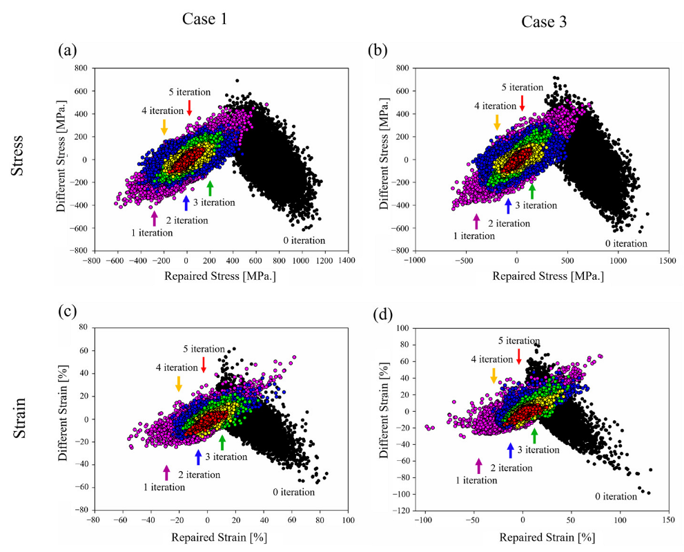
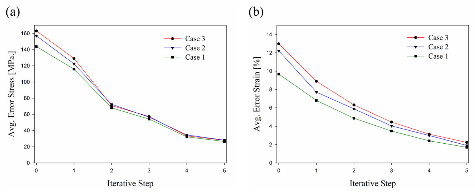
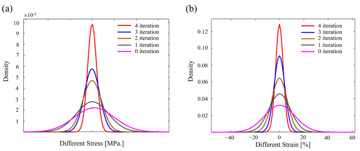
4.3. Convergence and Statistical Analysis

A quantitative analysis method determines the convergent behavior and confirms the error analysis via different iterative steps. The function of average difference is defined as follows:

$$e{r}_{\mathrm{avg}.}(x)={\displaystyle \sum _{\mathrm{i}=1}^{\mathrm{n}}\frac{\left|f_{\mathrm{ermi}}\right|}{n}}\mathrm{m}=0,1,2\dots , \mathrm{n}=10,000$$

(15)

where $f_{\mathrm{ermi}}$ is the difference in stress/strain between 3D and revised 2D layer results as derived in Equation (14), which can also be obtained by the magnitude of the y-axis in Figure 4, “m” is an iterative step from 0 to 5, and n is element number in 100 × 100 voxels RVEs. Figure 5 shows the average difference in stress/strain with different iterative steps. To avoid confusion, only case 1 to case 3 are shown in the convergence analysis. As can be seen, the convergent behavior with a small error is observed in the fourth iterative step. Therefore, it can be concluded that the fourth iterative step can reach the desired 3D local stress/strain distribution after almost 70% average difference in stress/strain conditions.

Previously presented qualitative comparisons of transformation are mainly based on individual visual perceptions. An appropriate statistical quantitative analysis is carried out here to compare the transformation results more accurately. For the statistical method, the probability distribution function is adopted. The probability distribution function can be derived in terms of $\mu$ and $\sigma$ as follows:

$$p(x)=\frac{1}{\sigma \sqrt{2\pi }}\exp (-\frac{{(x-\mu )}^2}{2{\sigma }^2}),\hspace{1em}\hspace{1em}-\infty <x<\infty$$

(16)

where $\mu$ is mean value of the probability distribution function $\sigma$ is the standard deviation value. The standard normal distribution-based probability distribution function of the difference in stress/strain distribution for case 1 with different iterative steps is shown in Figure 6. Note that five different stress/strains from zero to the fourth iterative step have been considered in the probability distribution function. Again, the different stress/strain comes from the general form in Equation (14), where the 2D revised stress/strain compared with 3D stress/strain is computed for each solution point. It can be seen that the peak considerably protrudes with the increase in iterative steps in the probability diagram. Therefore, it can be concluded that the error is convergent as iterative steps increases, which represents the derived 3D stress and strain distribution, as effectively calculated by the proposed iterative method.

4.4. Derivation of 3D Stress and Strain Distribution from the 2D Result

The graphic of derived 3D local stress and strain distribution with different iterative steps using the identified iterative constants will be demonstrated in this section. Due to the convergence and statistical analysis in Figure 5 and Figure 6, the transformation is carried out up to the fourth iterative step. Local stress/strain distribution for the revised 2D layer result, 3D layer result, and differences between 2D and 3D layer results for the ferrite phase of case 1 with different iterative steps is as displayed in Figure 7. In the first iteration, the stress/strain distribution displays the virtually perfectly averaged arrangement when forcibly applying a negative value on a larger stress/strain value and a positive value on a smaller stress/strain value by modification from corresponding $a_1$ and $b_1$ in Table 3 and Table 4. The high stress/strain zones disappear from the actual results. However, the difference in stress/strain between the first revised 2D and 3D layers can still be easily identified. The second revised stress/strain is obtained for the second iteration after modifying the first revised result by corresponding $a_2$ and $b_2$ in Table 3 and Table 4. It can be observed that the stress/strain concentration is generated along with the ferrite/martensite interfaces. The second iteration result displays a dramatic difference compared with the first iteration result. Subsequently, the third and fourth revised stress/strain are obtained during the modification of the second and third results revised by the corresponding $a_3$ and $b_3$ as well as $a_4$ and $b_4$ in Table 3 and Table 4. It can be seen that stress/strain concentration along the interface of the fourth revised result is more enhanced than the second revised result. It can be concluded that the derived 3D stress/strain distribution closely resembles the 3D result at the fourth iterative step.

5. Discussion

Due to the significantly higher stiffness of the martensite phase and strong “elastic mismatch” in the DP steels, higher interfacial stresses are induced due to applied mechanical or thermal loading [44,45]. Therefore, when comparing the stress and strain fields of the martensite and ferrite phases, extremely higher stress (≈2500 MPa) and lower strain are achieved in the martensite phase. On the contrary, smaller stress (≈800 MPa) and larger strain can be identified in the ferrite phase.

From the current and previous studies [28,37,38,46,47], in 2D crystal plasticity simulation, the obvious stress and strain concentrations exist in the ferrite phase due to the absence of the third dimension. As depth increases, the stress and strain are more distributed, and the concentration generally transfers to the matrix/particle interfaces and triple points of grains with a low Schmidt factor. As the thickness increases, the matrix’s stress field is phenomenally influenced by the adjacent inclusion. Chao et al. [48] indicated that the distance between two circular inclusions strongly provoked the stress field of the matrix and then interfered with the stress intensity factor of the crack.

Additionally, Diehl et al. [28] investigated the interaction between stress/strain conditions, the phase distribution of neighboring grain, and their crystallographic orientation. It was concluded that there is a drastic difference in local stress/strain distribution between 2D and 3D-RVEs results, which means it is difficult to validate simulation results with similar experiments. If 3D geometry is measured by slicing the surface, there is no same specimen available for the in situ tests. On the contrary, if the specimen is tested by deformation loading, 2D EBSD only can be obtained, and the corresponding 2D simulation result differs from the 3D distributions [28].

In the database of parameters from the proposed iterative method, as displayed in Table 3 and Table 4, it can be examined that the $R_m^2$ is practically similar in the same iterative step for ferrite phases regardless of total grain numbers, strain levels, and volume fractions. Additionally, the constants $a_m$ and $b_m$ nearly have a consistency tendency regardless of total grain numbers and volume fractions. There is a difference in the case of strain levels. That is, the constant $a_m$ and $R_m^2$ display a similar value for different strain levels. Conversely, the constants $b_m$ demonstrates larger value at larger strain levels. It is exhilarating that the 3D distribution can be straightforwardly responded to by 2D result by the same iterative constant owing to the similar $a_m$, $b_m$ and statistical analysis, which means that the 3D distribution can be derived by the proposed iterative method regardless of total grain numbers and volume fractions.

The methodology of deriving 3D local distribution from 2D results has been thoroughly introduced. In the future, the constants $a_m$ and $b_m$ can provide a helpful suggestion to predict the 3D local stress/strain from 2D local stress/strain. Henceforward, the derived 3D local stress and strain distribution can be an excellent validation of the experiment and further recommends the optimal design of the multiple phase steel with different grain orientation, total grain numbers, composition, and loading conditions by the proposed iterative method.

6. Conclusions

In this article, the derived crystal plasticity simulation of 3D local stress and strain has been successfully obtained from the 2D simulation result. The difference in the local stress and strain distributions in 2D and 3D simulations of the same surface is significant. There are three different parameter series, including total grain numbers, strain levels, and volume fractions. After identifying the difference in the local distributions, the alternative error and least square methods are used to transform the 2D results to match with 3D observations. It is shown that using the presented proposed iterative technique, the 3D distribution can be quickly derived from the 2D result in a ferrite matrix of DP steel. It can be concluded that the desired transformation can be achieved in the fourth iterative step by using the identified iterative constants for each phase. For the iterative constants, almost similar values regardless of total grain numbers and volume fractions are displayed. The accuracy of the developed method is demonstrated by visual and statistical analysis, and the proposed numerical approach can be regarded as effective and efficient. In the future, this method can be applied to forecast 3D distributions of stress and strain in other multiphase materials, such as spheroidized steels and particle-based metal composites.

References

1. Tasan, C.C.; Diehl, M.; Yan, D.; Bechtold, M.; Roters, F.; Schemmann, L.; Zheng, C.; Peranio, N.; Ponge, D.; Koyama, M.; et al. An overview of dual-phase steels: Advances in microstructure-oriented processing and micromechanically guided design. Annu. Rev. Mater. Res. 2015, 45, 391–431. [Google Scholar] [CrossRef]
2. Hussein, T.; Umar, M.; Qayyum, F.; Guk, S.; Prahl, U. Micromechanical Effect of Martensite Attributes on Forming Limits of Dual-Phase Steels Investigated by Crystal Plasticity-Based Numerical Simulations. Crystals 2022, 12, 155. [Google Scholar] [CrossRef]
3. Biermann, H.; Martin, U.; Aneziris, C.G.; Kolbe, A.; Müller, A.; Schärfl, W.; Herrmann, M. Microstructure and compression strength of novel TRIP-steel/Mg-PSZ composites. Adv. Eng. Mater. 2009, 11, 1000–1006. [Google Scholar] [CrossRef]
4. Biermann, H.; Aneziris, C.G. Austenitic TRIP/TWIP Steels and Steel-Zirconia Composites: Design of Tough, Transformation-Strengthened Composites and Structures; Springer Nature: Berlin/Heidelberg, Germany, 2020; Volume 298. [Google Scholar]
5. Asghar, W.; Nasir, M.A.; Qayyum, F.; Shah, M.; Azeem, M.; Nauman, S.; Khushnood, S. Investigation of fatigue crack growth rate in CARALL, ARALL and GLARE. Fatigue Fract. Eng. Mater. Struct. 2017, 40, 1086–1100. [Google Scholar] [CrossRef]
6. Khan, F.; Qayyum, F.; Asghar, W.; Azeem, M.; Anjum, Z.; Nasir, A.; Shah, M. Effect of various surface preparation techniques on the delamination properties of vacuum infused Carbon fiber reinforced aluminum laminates (CARALL): Experimentation and numerical simulation. J. Mech. Sci. Technol. 2017, 31, 5265–5272. [Google Scholar] [CrossRef]
7. Qayyum, F.; Kamran, A.; Ali, A.; Shah, M. 3D numerical simulation of thermal fatigue damage in wedge specimen of AISI H13 tool steel. Eng. Fract. Mech. 2017, 180, 240–253. [Google Scholar] [CrossRef]
8. Mukhtar, F.; Qayyum, F.; Shah, M. Studying the effect of thermal fatigue on multiple cracks propagating in an SS316L thin flange on a shaft specimen using a multi-physics numerical simulation model. J. Mech. Eng. 2019, 65, 565–573. [Google Scholar] [CrossRef]
9. Hussain, N.; Qayyum, F.; Pasha, R.A.; Shah, M. Development of multi-physics numerical simulation model to investigate thermo-mechanical fatigue crack propagation in an autofrettaged gun barrel. Def. Technol. 2020, 17, 1579–1591. [Google Scholar] [CrossRef]
10. Ibrahim, I.; Mohamed, F.; Lavernia, E. Particulate reinforced metal matrix composites—A review. J. Mater. Sci. 1991, 26, 1137–1156. [Google Scholar] [CrossRef]
11. Kanouté, P.; Boso, D.P.; Chaboche, J.L.; Schrefler, B. Multiscale methods for composites: A review. Arch. Comput. Methods Eng. 2009, 16, 31–75. [Google Scholar] [CrossRef]
12. Hannard, F.; Simar, A.; Maire, E.; Pardoen, T. Quantitative assessment of the impact of second phase particle arrangement on damage and fracture anisotropy. Acta Mater. 2018, 148, 456–466. [Google Scholar] [CrossRef]
13. Zhang, J.F.; Zhang, X.X.; Wang, Q.Z.; Xiao, B.L.; Ma, Z.Y. Simulations of deformation and damage processes of SiCp/Al composites during tension. J. Mater. Sci. Technol. 2018, 34, 627–634. [Google Scholar] [CrossRef]
14. Lee, S.B.; Lebensohn, R.; Rollett, A.D. Modeling the viscoplastic micromechanical response of two-phase materials using Fast Fourier Transforms. Int. J. Plast. 2011, 27, 707–727. [Google Scholar] [CrossRef]
15. Lebensohn, R.A.; Kanjarla, A.K.; Eisenlohr, P. An elasto-viscoplastic formulation based on fast Fourier transforms for the prediction of micromechanical fields in polycrystalline materials. Int. J. Plast. 2012, 32–33, 59–69. [Google Scholar] [CrossRef]
16. Fujita, N.; Igi, S.; Diehl, M.; Roters, F.; Raabe, D. The through-process texture analysis of plate rolling by coupling finite element and fast Fourier transform crystal plasticity analysis. Model. Simul. Mater. Sci. Eng. 2019, 27, 085005. [Google Scholar] [CrossRef]
17. Kanit, T.; Forest, S.; Galliet, I.; Mounoury, V.; Jeulin, D. Determination of the size of the representative volume element for random composites: Statistical and numerical approach. Int. J. Solids Struct. 2003, 40, 3647–3679. [Google Scholar] [CrossRef]
18. Kadkhodapour, J.; Butz, A.; Ziaei-Rad, S.; Schmauder, S. A micro mechanical study on failure initiation of dual phase steels under tension using single crystal plasticity model. Int. J. Plast. 2011, 27, 1103–1125. [Google Scholar] [CrossRef]
19. Uthaisangsuk, V.; Prahl, U.; Bleck, W. Stretch-flangeability characterisation of multiphase steel using a microstructure based failure modelling. Comput. Mater. Sci. 2009, 45, 617–623. [Google Scholar] [CrossRef]
20. Bargmann, S.; Klusemann, B.; Markmann, J.; Schnabel, J.E.; Schneider, K.; Soyarslan, C.; Wilmers, J. Generation of 3D representative volume elements for heterogeneous materials: A review. Prog. Mater. Sci. 2018, 96, 322–384. [Google Scholar] [CrossRef]
21. Groeber, M.; Ghosh, S.; Uchic, M.D.; Dimiduk, D.M. A framework for automated analysis and simulation of 3D polycrystalline microstructures.: Part 1: Statistical characterization. Acta Mater. 2008, 56, 1257–1273. [Google Scholar] [CrossRef]
22. Groeber, M.; Ghosh, S.; Uchic, M.D.; Dimiduk, D.M. A framework for automated analysis and simulation of 3D polycrystalline microstructures. Part 2: Synthetic structure generation. Acta Mater. 2008, 56, 1274–1287. [Google Scholar] [CrossRef]
23. Diehl, M.; Groeber, M.; Haase, C.; Molodov, D.A.; Roters, F.; Raabe, D. Identifying structure–property relationships through DREAM. 3D representative volume elements and DAMASK crystal plasticity simulations: An integrated computational materials engineering approach. Jom 2017, 69, 848–855. [Google Scholar] [CrossRef] [Green Version]
24. Roters, F.; Diehl, M.; Shanthraj, P.; Eisenlohr, P.; Reuber, C.; Wong, S.L.; Maiti, T.; Ebrahimi, A.; Hochrainer, T.; Fabritius, H.O.; et al. DAMASK–The Düsseldorf Advanced Material Simulation Kit for modeling multi-physics crystal plasticity, thermal, and damage phenomena from the single crystal up to the component scale. Comput. Mater. Sci. 2019, 158, 420–478. [Google Scholar] [CrossRef]
25. Ramazani, A.; Mukherjee, K.; Quade, H.; Prahl, U.; Bleck, W. Correlation between 2D and 3D flow curve modelling of DP steels using a microstructure-based RVE approach. Mater. Sci. Eng. A 2013, 560, 129–139. [Google Scholar] [CrossRef]
26. Qayyum, F.; Guk, S.; Prüger, S.; Schmidtchen, M.; Saenko, I.; Kiefer, B.; Kawalla, R.; Prahl, U. Investigating the local deformation and transformation behavior of sintered X3CrMnNi16-7-6 TRIP steel using a calibrated crystal plasticity-based numerical simulation model. Int. J. Mater. Res. 2020, 111, 392–404. [Google Scholar] [CrossRef]
27. Qayyum, F.; Guk, S.; Schmidtchen, M.; Kawalla, R.; Prahl, U. Modeling the local deformation and transformation behavior of cast X8CrMnNi16-6-6 TRIP steel and 10% Mg-PSZ composite using a continuum mechanics-based crystal plasticity model. Crystals 2020, 10, 221. [Google Scholar] [CrossRef] [Green Version]
28. Diehl, M.; Shanthraj, P.; Eisenlohr, P.; Roters, F. Neighborhood influences on stress and strain partitioning in dual-phase microstructures. Meccanica 2016, 51, 429–441. [Google Scholar] [CrossRef]
29. Qayyum, F.; Guk, S.; Prahl, U. Studying the damage evolution and the micro-mechanical response of X8CrMnNi16-6-6 TRIP steel matrix and 10% zirconia particle composite using a calibrated physics and crystal-plasticity-based numerical simulation model. Crystals 2021, 11, 759. [Google Scholar] [CrossRef]
30. Qayyum, F.; Guk, S.; Kawalla, R.; Prahl, U. Experimental Investigations and Multiscale Modeling to Study the Effect of Sulfur Content on Formability of 16MnCr5 Alloy Steel. Steel Res. Int. 2018, 90, 1800369. [Google Scholar] [CrossRef]
31. Sedighiani, K.; Traka, K.; Roters, F.; Raabe, D.; Sietsma, J.; Diehl, M. Determination and analysis of the constitutive parameters of temperature-dependent dislocation-density-based crystal plasticity models. Mech. Mater. 2022, 164, 104117. [Google Scholar] [CrossRef]
32. Sedighiani, K.; Diehl, M.; Traka, K.; Roters, F.; Sietsma, J.; Raabe, D. An efficient and robust approach to determine material parameters of crystal plasticity constitutive laws from macro-scale stress–strain curves. Int. J. Plast. 2020, 134, 102779. [Google Scholar] [CrossRef]
33. Weidner, A.; Biermann, H. Review on Strain Localization Phenomena Studied by High-Resolution Digital Image Correlation. Adv. Eng. Mater. 2021, 23, 2001409. [Google Scholar] [CrossRef]
34. Weidner, A.; Biermann, H. Combination of Different In Situ Characterization Techniques and Scanning Electron Microscopy Investigations for a Comprehensive Description of the Tensile Deformation Behavior of a CrMnNi TRIP/TWIP Steel. Jom 2015, 67, 1729–1747. [Google Scholar] [CrossRef]
35. Weidner, A.; Berek, H.; Segel, C.; Aneziris, C.G.; Biermann, H. In situ tensile deformation of TRIP steel/Mg-PSZ composites. Mater. Sci. Forum 2013, 738–739, 77–81. [Google Scholar] [CrossRef]
36. Vinogradov, A.; Lazarev, A.; Linderov, M.; Weidner, A.; Biermann, H. Kinetics of deformation processes in high-alloyed cast transformation-induced plasticity/twinning-induced plasticity steels determined by acoustic emission and scanning electron microscopy: Influence of austenite stability on deformation mechanisms. Acta Mater. 2013, 61, 2434–2449. [Google Scholar] [CrossRef]
37. Qayyum, F.; Chaudhry, A.A.; Guk, S.; Schmidtchen, M.; Kawalla, R.; Prahl, U. Effect of 3D Representative Volume Element (RVE) Thickness on Stress and Strain Partitioning in Crystal Plasticity Simulations of Multi-Phase Materials. Crystals 2020, 10, 944. [Google Scholar] [CrossRef]
38. Qayyum, F.; Umar, M.; Guk, S.; Schmidtchen, M.; Kawalla, R.; Prahl, U. Effect of the 3rd Dimension within the Representative Volume Element (RVE) on Damage Initiation and Propagation during Full-Phase Numerical Simulations of Single and Multiphase Steels. Materials 2021, 14, 42. [Google Scholar] [CrossRef]
39. Umar, M.; Qayyum, F.; Farooq, M.U.; Guk, S.; Kirschner, M.; Korpala, G.; Prahl, U. Exploring the Structure–Property Relationship in Spheroidized C45EC Steel Using Full Phase Crystal Plasticity Numerical Simulations. Steel Res. Int. 2022, 93, 2100452. [Google Scholar] [CrossRef]
40. Qayyum, F.; Umar, M.; Elagin, V.; Kirschner, M.; Hoffmann, F.; Guk, S.; Prahl, U. Influence of Non-Metallic Inclusions on Local Deformation and Damage Behavior of Modified 16MnCrS5 Steel. Crystals 2022, 12, 281. [Google Scholar] [CrossRef]
41. Umar, M.; Qayyum, F.; Farooq, M.U.; Khan, L.A.; Guk, S.; Prahl, U. Analyzing the cementite particle size and distribution in heterogeneous microstructure of C45EC steel using crystal plasticity based DAMASK code. In Proceedings of the 2021 International Bhurban Conference on Applied Sciences and Technologies (IBCAST), Islamabad, Pakistan, 12–16 January 2021; pp. 15–20. [Google Scholar]
42. Jiang, Z.; Guan, Z.; Lian, J. Effects of microstructural variables on the deformation behaviour of dual-phase steel. Mater. Sci. Eng. A 1995, 190, 55–64. [Google Scholar] [CrossRef]
43. Eisenlohr, P.; Diehl, M.; Lebensohn, R.A.; Roters, F. A spectral method solution to crystal elasto-viscoplasticity at finite strains. Int. J. Plast. 2013, 46, 37–53. [Google Scholar] [CrossRef]
44. Tseng, S.C.; Chao, C.K.; Chen, F.M.; Chiu, W.C. Interfacial stresses of a coated polygonal hole subject to a point heat source. J. Therm. Stresses. 2020, 43, 1487–1512. [Google Scholar] [CrossRef]
45. Tseng, S.C.; Chao, C.K.; Chen, F.M. Interfacial stresses of a coated square hole induced by a remote uniform heat flow. International J. Appl. Mech. 2020, 12, 2050063. [Google Scholar] [CrossRef]
46. Diehl, M.; Naunheim, Y.; Yan, D.; Morsdorf, L.; An, D.; Tasan, C.C.; Zaefferer, S.; Roters, F.; Raabe, D. Coupled Experimental-Numerical Analysis of Strain Partitioning in Metallic Microstructures: The Importance of Considering the 3D Morphology. In Proceedings of the BSSM 12th International Conference on Advances in Experimental Mechanics, Sheffield, UK, 29–31 August 2017; pp. 1–2. [Google Scholar]
47. Diehl, M.; An, D.; Shanthraj, P.; Zaefferer, S.; Roters, F.; Raabe, D. Crystal plasticity study on stress and strain partitioning in a measured 3D dual phase steel microstructure. Phys. Mesomech. 2017, 20, 311–323. [Google Scholar] [CrossRef]
48. Chao, C.K.; Tseng, S.C.; Chen, F.M. Mode-III stress intensity factors for two circular inclusions subject to a remote uniform shear load. J. Chin. Inst. Eng. 2018, 41, 590–602. [Google Scholar] [CrossRef]
Figure 1. The schematic diagram represents the flow chart of the current work. The upper half (yellow background) indicates the flow chart of crystal simulation, and the bottom half (blue background) represents numerical analysis. The blue arrow indicates the flow of data. The red arrow represents tensile loading, and the yellow arrow separates the ferrite (F) and martensite (M) phases.
Crystals 12 00955 g001
Figure 2. (a) The resulting RVE-C initial microstructure colored according to the inverse pole figure (IPF). (b) All RVE models (RVE-A to RVE-F) were sliced into geometries with 1-layer (h = 0.01) RVE in terms of texture style.
Crystals 12 00955 g002
Figure 3. Local von Mises stress and strain distribution for ferrite phase from case 1 to case 9. Note that case 1 to case 3 indicate different total grain numbers; case 4 to case 6 indicate different strain levels; case 7 to case 9 indicate different volume fractions. The extreme left and right column indicates the 2D and 3D local stress and strain distribution differences, respectively.
Crystals 12 00955 g003
Figure 4. Scatter diagram showing the numerical tendency of stress in (a) case 1 (b) case 3 and strain in (c) case 1 (d) case 3 by the proposed iterative method for ferrite phase at 25% global true strain and 0.1 volume fraction.
Crystals 12 00955 g004
Figure 5. Convergence analysis for the ferrite phase at 25% global true strain. (a) Stress and (b) strain by the proposed iterative method with different iterative steps.
Crystals 12 00955 g005
Figure 6. Probability distribution function of different (a) stress and (b) strain distributions between 3D result and iteratively revised 2D result for the ferrite phase of case 1 with different iterative steps.
Crystals 12 00955 g006
Figure 7. Local von Mises stress and strain distribution for the ferrite phase of case 1 with different iterative steps. The extreme left and right column indicate the 2D and 3D local stress and strain distribution differences, respectively.
Crystals 12 00955 g007