Article

Piezoelectric Resonators Excited by Lateral Electric Fields Based on a LiTaO3 Single Crystal

1
Piezoelectric Device Laboratory, School of Mechanical Engineering and Mechanics, Ningbo University, Ningbo 315211, China
2
Institute of Acoustics, the Chinese Academy of Sciences, Beijing 100190, China
*
Authors to whom correspondence should be addressed.
Crystals 2020, 10(6), 525; https://doi.org/10.3390/cryst10060525
Submission received: 25 May 2020 / Revised: 14 June 2020 / Accepted: 15 June 2020 / Published: 18 June 2020

Abstract

:
In the present study, piezoelectric resonators under lateral field excitation (LFE) based on a LiTaO3 single crystal are modeled and analyzed. An electrically forced vibration study is employed to acquire the motional capacitance curve and vibration mode shapes. A finite element approach is utilized to investigate the influences of some basic parameters, such as the electrode/plate mass ratio, electrode gap, and electrode width on resonance characteristics. In addition, the design criteria for the gap and width of the electrode of the LiTaO3 LFE resonators are obtained by analyzing the effects of those parameters on vibration strain distributions. The obtained results are essential for designing LFE piezoelectric resonators by using a LiTaO3 single crystal.

1. Introduction

Piezoelectric crystal resonators have been extensively employed for frequency production and control, telecommunication, and sensing [1,2,3,4,5,6,7]. Lateral field excitation (LFE)-based piezoelectric crystal resonators, adopting two electrodes on a surface of the piezoelectric substrate, are known as useful sensing tools with a number of advantages. Higher quality factor (Q-factor), superior frequency stability, and high durability have made LFE devices more suitable for sensing compared with conventional thickness field excitation (TFE) devices [8,9,10,11,12]. In addition, more effective data about analytes obtained by LFE sensors provide a valuable tool for sensing and the evaluation of reaction procedures in biochemical systems [13,14].
For the conventional resonators based on AT-cut quartz crystals, the small value of the piezoelectric coupling coefficient makes the quality factor (Q-factor) under large damps low, resulting in the frequency stability not being enough [15]. The bulk acoustic wave devices with strong piezoelectric couplings can obtain a high Q-factor under a large damping [16]. The 3m point group single crystal LiTaO3 has high piezoelectric constants [17]; thus, the LFE devices based on a LiTaO3 single crystal are appropriate for sensing applications, with significant damping. In addition, the LFE devices employing a LiTaO3 single crystal can also obtain a higher sensitivity to electrical properties because of the higher piezoelectric coupling coefficients.
The theoretical model of traditional quartz crystal LFE devices was built by Yang [18]. The studies performed in [18] were mainly for demonstrating the concept. A pair of non-realistic side electrodes at the edges of thin crystal plates were employed in [18] to generate the lateral electric field. Usually, in actual devices, a pair of electrodes at the top (or bottom) of the plate’s surface are utilized to generate the lateral electric field [19,20]. Presently, the vibration analysis model of the LFE device using a 3m point group single crystal operating in air is scarce, and the vibration strain distributions of the devices are more complex, due to the lateral electrical fields generated by surface electrodes and the stronger piezoelectric coupling. In addition, the influences of size factors of the crystal plate and the electrodes on the vibration characteristics are unclear, which hinders the optimal design of the LFE resonators using a LiTaO3 single crystal.
In this paper, the theoretical model of LiTaO3 resonators stimulated by lateral electric fields is built using the Mindlin plate theory. The electrically forced vibrations of the resonators are studied. The impact of various structural factors on the resonators is revealed. The finite element analysis is utilized to verify the theoretical results. Based on the analyses, the design criteria for the gap and width of the electrodes are obtained.

2. Governing Equation

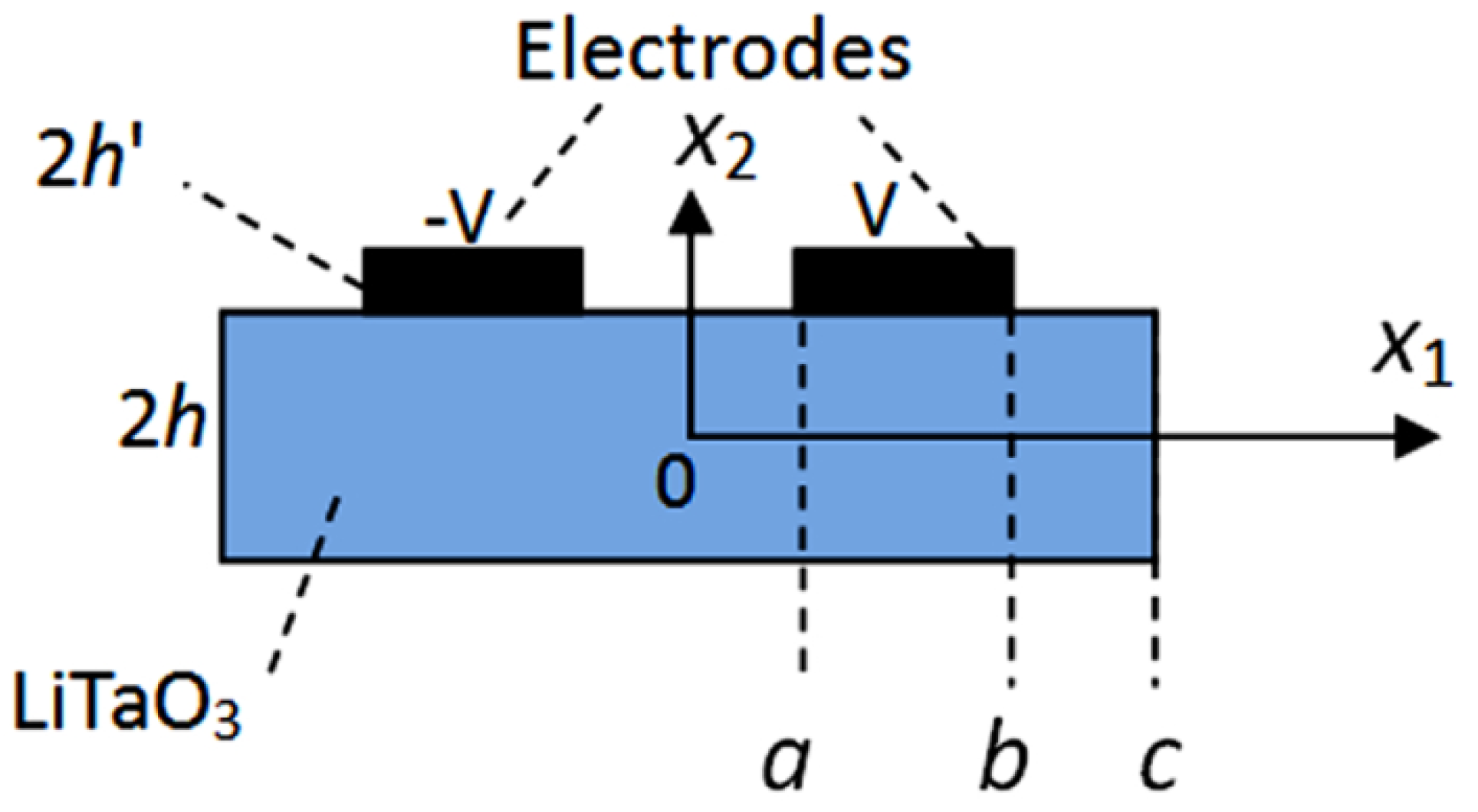
A rectangular (yxl) 90° LiTaO3 crystal plate is considered (see Figure 1). The cut orientation (yxl) 90° can be used for LiTaO3 resonators working on pure-LFE mode with a high piezoelectric coupling factor (44.52%) [21], thus the (yxl) 90° crystal cut is selected. A plate with a 2h thickness and a mass density of ρ is considered. For the crystal plate with a (yxl) 90° cut orientation, the crystallographic z-axis is parallel to the x 2 axis, the crystallographic x-axis is parallel to the x 1 axis, and the crystallographic y-axis is parallel to the x 3 axis.
The plate is symmetric at about x 1 = 0. It is infinite in the x 3 axis and does not change along with it. In the range of a < | x 1 | < b , two electrodes are positioned on the top surface of the plate, where their thickness and density are indicated by 2h′ and ρ , respectively. A time-harmonic supply voltage ± V exp(iωt) is exerted to the two electrodes, which generates an electrical field with a primary component E 1 ( x 1 , t ) in the middle area without any electrode. Since the LiTaO3 crystal is particularly anisotropic, the vibrations of the thickness-shear (TSh) mode, the face-shear (FS) mode and the flexural (F) mode are coupled in the crystal plate. Both the TSh and F modes are excited through piezoelectric constant e16, and the FS mode is excited by piezoelectric constant e15.
Mindlin’s plate equations for plates with or without electrodes are different. These equations are given in the following. In the plate without the electrode, the corresponding displacements and electric potentials of the coupled TSh, FS and F motions can be approximated as follows [9,22]:
u 1 x 2 u 1 ( 1 ) ( x 1 , t ) , u 2 u 2 ( 0 ) ( x 1 , t ) , u 3 u 3 ( 0 ) ( x 1 , t ) , ϕ ϕ ( 0 ) ( x 1 , t ) ,
where the FS displacement, the F displacement, and the TSh displacement are denoted by u 3 ( 0 ) ( x 1 , t ) , u 2 ( 0 ) ( x 1 , t ) , and u 1 ( 1 ) ( x 1 , t ) , respectively. ϕ ( 0 ) is the electric potential. The TSh mode, as the high frequency operation mode of the resonator, is coupled with the FS mode and the F mode by the elastic constant c65, c66, respectively. The governing equations for u 3 ( 0 ) , u 2 ( 0 ) , u 1 ( 1 ) and ϕ ( 0 ) are:
T 6 , 1 ( 0 ) = 2 h ρ u ¨ 2 ( 0 ) T 5 , 1 ( 0 ) = 2 h ρ u ¨ 3 ( 0 ) T 1 , 1 ( 1 ) T 6 ( 0 ) = 2 h 3 3 ρ u ¨ 1 ( 1 ) D 1 ( 0 ) = 0
In (2), the face-traction T 6 ( 0 ) , T 5 ( 0 ) , T 1 ( 1 ) and face-charge D 1 ( 0 ) are given by the following constitutive equation:
T 6 ( 0 ) = 2 h [ k 1 c 65 u 3 , 1 ( 0 ) + k 1 2 c 66 ( u 2 , 1 ( 0 ) + u 1 ( 1 ) ) + k 1 e 16 ϕ , 1 ( 0 ) ] T 5 ( 0 ) = 2 h [ c 55 u 3 , 1 ( 0 ) + k 1 c 56 ( u 2 , 1 ( 0 ) + u 1 ( 1 ) ) + e 15 ϕ , 1 ( 0 ) ] T 1 ( 1 ) = 2 h 3 3 [ γ 11 u 1 , 1 ( 1 ) ] D 1 ( 0 ) = 2 h [ e 15 u 3 , 1 ( 0 ) + k 1 e 16 ( u 2 , 1 ( 0 ) + u 1 ( 1 ) ) ε 11 ϕ , 1 ( 0 ) ]
where
γ 11 = s 33 s 11 s 33 s 31 2 ,   k 1 2 = π 2 12
c p q ( = c p q E ) , e i p and ε i j ( = ε i j S ) are elastic stiffness, piezoelectric constant and dielectric constant, respectively. Inserting (3) into (2) leads to these three displacement and potential equations:
k 1 c 65 u 3 , 11 ( 0 ) + k 1 2 c 66 u 2 , 11 ( 0 ) + k 1 2 c 66 u 1 , 1 ( 1 ) + k 1 e 16 ϕ , 11 ( 0 ) = ρ u ¨ 2 ( 0 ) , c 55 u 3 , 11 ( 0 ) + k 1 c 56 u 2 , 11 ( 0 ) + k 1 c 56 u 1 , 1 ( 1 ) + e 15 ϕ , 11 ( 0 ) = ρ u ¨ 3 ( 0 ) , γ 11 u 1 , 11 ( 1 ) 3 h 2 [ k 1 c 65 u 3 , 1 ( 0 ) + k 1 2 c 66 u 2 , 1 ( 0 ) + k 1 2 c 66 u 1 ( 1 ) + k 1 e 16 ϕ , 1 ( 0 ) ] = ρ u ¨ 1 ( 0 ) , e 15 u 3 , 11 ( 0 ) + k 1 e 16 ( u 2 , 11 ( 0 ) + u 1 , 1 ( 1 ) ) ε 11 ϕ , 11 ( 0 ) = 0 .
In the electroded area of the plate, the electric potential ϕ ( 0 ) could be considered as a constant and Equation (2)4 can be omitted. For Equation (2)1,2,3, the influence of the electrode mass should be considered. The equations take the following form:
T 6 , 1 ( 0 ) = 2 h ρ ( 1 + R ) u ¨ 2 ( 0 ) , T 5 , 1 ( 0 ) = 2 h ρ ( 1 + R ) u ¨ 3 ( 0 ) , T 1 , 1 ( 1 ) T 6 ( 0 ) = 2 h 3 3 ρ ( 1 + 3 R ) u ¨ 1 ( 1 ) ,
where the electrode/plate mass ratio is R = ρ h / ρ h < < 1 , the constitutive equations of the electroded region are:
T 6 ( 0 ) = 2 h [ k ¯ 1 c 65 u 3 , 1 ( 0 ) + k ¯ 1 2 c 66 ( u 2 , 1 ( 0 ) + u 1 ( 1 ) ) ] , T 5 ( 0 ) = 2 h [ c 55 u 3 , 1 ( 0 ) + k ¯ 1 c 56 ( u 2 , 1 ( 0 ) + u 1 ( 1 ) ) ] , T 1 ( 1 ) = 2 h 3 3 [ γ 11 u 1 , 1 ( 1 ) ] ,
where k ¯ 1 2 = k 1 2 ( 1 + R ) .
Substitution (7) into (6) gives the following equations:
k ¯ 1 c 65 u 3 , 11 ( 0 ) + k ¯ 1 2 c 66 u 2 , 11 ( 0 ) + k ¯ 1 2 c 66 u 1 , 1 ( 1 ) = ρ ( 1 + R ) u ¨ 2 ( 0 ) , c 55 u 3 , 11 ( 0 ) + k ¯ 1 c 56 u 2 , 11 ( 0 ) + k ¯ 1 c 56 u 1 , 1 ( 1 ) = ρ ( 1 + R ) u ¨ 3 ( 0 ) , γ 11 u 1 , 11 ( 1 ) 3 h 2 [ k ¯ 1 c 65 u 3 , 1 ( 0 ) + k ¯ 1 2 c 66 u 2 , 1 ( 0 ) + k ¯ 1 2 c 66 u 1 ( 1 ) ] = ρ ( 1 + 3 R ) u ¨ 1 ( 1 ) .

3. Dispersion Characteristics

Examining the dispersion relations of waves in unbounded plates is useful for understanding resonator behaviors. Let the wave frequency be ω and the wave number along x1 be ξ . For an unelectroded plate, consider the possibility of the following wave:
u 2 ( 0 ) = A 1 sin ( ξ x 1 ω t ) , u 3 ( 0 ) = A 2 sin ( ξ x 1 ω t ) , u 1 ( 1 ) = A 3 cos ( ξ x 1 ω t ) , ϕ ( 0 ) = A 4 sin ( ξ x 1 ω t ) ,
where A1A4 are undetermined constants. (9) is substituted to (5), and then four linear homogeneous equations for A1A4 are obtained. The determinant of the coefficient matrix has to vanish for nontrivial solutions, which yields an equation that determines ω versus ξ , namely, the dispersion relation of the wave. Similarly, for an electroded plate with a grounded electrode, ϕ ( 0 ) = 0 . The corresponding dispersion relations can be obtained by substituting the u 2 ( 0 ) , u 3 ( 0 ) and u 1 ( 1 ) from (9) into (8). The following dimensionless frequency Ω and dimensionless wave number X are defined:
Ω = ω ω 0 ,   X = ξ / π 2 h ,   ω 0 = ( π / 2 h ) c 66 / ρ
where ω 0 is the fundamental TSh frequency of an unelectroded plate and is used as a normalizing frequency. Dispersion relations for both electroded (dotted lines) and unelectroded (solid lines) plates are shown in Figure 2. As expected, the electroded plate has lower frequencies due to the electrode inertia. The branch for the TSh wave has a finite intercept with the vertical or frequency (Ω) axis, which is the cutoff frequency below which the TSh wave cannot propagate.

4. Electrically Forced Vibration of Finite Plates

Because the plate is symmetrical about x 1 = 0 and an anti-symmetric voltage is applied to the electroded plate, the electromechanical coupling fields could be symmetric or anti-symmetric, with respect to x 1 = 0 . In the current paper, we only consider the right half. Since the plate is partly covered by the electrode, separate solutions are required for areas with and without the electrode.

4.1. Central Area without the Electrode with 0 < x 1 < a

The following wave form is considered:
u 2 ( 0 ) = A 1 sin ( ξ x 1 ) e i ω t , u 3 ( 0 ) = A 2 sin ( ξ x 1 ) e i ω t , u 1 ( 1 ) = A 3 cos ( ξ x 1 ) e i ω t , ϕ ( 0 ) = A 4 sin ( ξ x 1 ) e i ω t ,
where A 1 A 4 are undetermined constants. Inserting (11) into (5) gives four linear relations for A 1 A 4 . The coefficient matrix determinant should be equal to zero for nontrivial solutions. This leads to a third-order equation in terms of ξ . This equation has three nonzero solutions represented by ξ ( m ) 2 , with m = 1–3. The nontrivial solution of the linear equation is denoted by β p ( m ) , with p = 1–4 corresponding to a ξ ( m ) . β p ( m ) indicates the ratios among A 1 A 4 . Now, the general solution of the equation could be written as:
{ u 2 ( 0 ) u 3 ( 0 ) u 1 ( 1 ) ϕ ( 0 ) } = m = 1 3 C ( m ) { β 1 ( m ) sin ( ξ ( m ) x 1 ) β 2 ( m ) sin ( ξ ( m ) x 1 ) β 3 ( m ) cos ( ξ ( m ) x 1 ) β 4 ( m ) sin ( ξ ( m ) x 1 ) } + C ( 4 ) { 0 0 B 1 x 1 } ,
where C ( 1 ) C ( 4 ) are unknown constants, and
B 1 = 3 h 2 k 1 e 16 3 h 2 k 1 2 c 66 ρ ω 2 ,
C ( 4 ) is constructed from the root of ξ 2 = 0 .

4.2. Area Including the Electrode with a < x 1 < b

In the area with the electrode, the applied electric potential is denoted by ϕ ( 0 ) . Let
u 2 ( 0 ) = A 1 e i ξ ¯ x 1 e i ω t , u 3 ( 0 ) = A 2 e i ξ ¯ x 1 e i ω t , u 1 ( 1 ) = A 3 e i ξ ¯ x 1 e i ω t ,
where A 1 A 3 are undetermined constants. (14) is substituted into (8), and then three linear equations for A 1 A 3 are obtained. The coefficient matrix determinant must be equal to zero for nontrivial solutions. This gives a third-order polynomial term of ξ ¯ 2 . This equation has six nonzero solutions indicated by ξ ¯ ( m ) , with m = 1–6. The nontrivial solution of the linear equation is denoted by β ¯ p ( m ) , with p = 1–3 corresponding to a ξ ¯ ( m ) . β ¯ p ( m ) indicates the ratios among A 1 A 3 . Now, the following expression could be obtained for the general solution of the equation:
{ u 2 ( 0 ) u 3 ( 0 ) u 1 ( 1 ) } = m = 1 6 C ¯ ( m ) { β ¯ 1 ( m ) e i ξ ¯ ( m ) x 1 β ¯ 2 ( m ) e i ξ ¯ ( m ) x 1 β ¯ 3 ( m ) e i ξ ¯ ( m ) x 1 } ,
where C ¯ ( 1 ) C ¯ ( 6 ) are unknown constants.

4.3. External Area without the Electrode with b < x 1 < c

Let
u 2 ( 0 ) = A 1 e i ξ ˜ x 1 e i ω t , u 3 ( 0 ) = A 2 e i ξ ˜ x 1 e i ω t , u 1 ( 1 ) = A 3 e i ξ ˜ x 1 e i ω t , ϕ ( 0 ) = A 4 e i ξ ˜ x 1 e i ω t ,
where A 1 A 4 are undetermined constants. (16) is substituted into (5), and then four linear equations for A 1 A 4 are obtained. To obtain the nontrivial solutions, the coefficient matrix determinant should be zero. This leads to a fourth-order equation in terms of ( ξ ˜ ) 2 . Accordingly, six nonzero roots are obtained, which are described by ξ ˜ ( m ) , m = 1–6. The nontrivial solution of the linear equation is denoted by β ˜ p ( m ) , with p = 1–4 corresponding to a ξ ˜ ( m ) . β ˜ p ( m ) indicates the ratios among A 1 A 4 . Now, the general solution of the equation could be described as:
{ u 2 ( 0 ) u 3 ( 0 ) u 1 ( 1 ) ϕ ( 0 ) } = m = 1 6 C ˜ ( m ) { β ˜ 1 ( m ) e i ξ ˜ ( m ) x 1 β ˜ 2 ( m ) e i ξ ˜ ( m ) x 1 β ˜ 3 ( m ) e i ξ ˜ ( m ) x 1 β ˜ 4 ( m ) e i ξ ˜ ( m ) x 1 } + C ( 7 ) { 0 0 B ˜ 1 x 1 } + C ( 8 ) { 0 0 0 1 } ,
where C ˜ ( 1 ) C ˜ ( 8 ) are unknown constants, and
B ˜ 1 = B 1 ,
C ˜ ( 7 ) C ˜ ( 8 ) is constructed from the root of ξ ˜ 2 = 0 .

4.4. Boundary and Continuous Conditions

The boundary and continuity conditions of the electrically forced vibration could be employed to determine the resonator motion capacitance. At x 1 = a , we have continuity conditions:
u 2 ( 0 ) ( x 1 = a ) = u 2 ( 0 ) ( x 1 = a + ) , u 3 ( 0 ) ( x 1 = a ) = u 3 ( 0 ) ( x 1 = a + ) , u 1 ( 1 ) ( x 1 = a ) = u 1 ( 1 ) ( x 1 = a + ) , T 6 ( 0 ) ( x 1 = a ) = T 6 ( 0 ) ( x 1 = a + ) , T 5 ( 0 ) ( x 1 = a ) = T 5 ( 0 ) ( x 1 = a + ) , T 1 ( 1 ) ( x 1 = a ) = T 1 ( 1 ) ( x 1 = a + ) , ϕ ( 0 ) ( x 1 = a ) = V e i ω t .
At x 1 = b , we have continuity conditions:
u 2 ( 0 ) ( x 1 = b ) = u 2 ( 0 ) ( x 1 = b + ) , u 3 ( 0 ) ( x 1 = b ) = u 3 ( 0 ) ( x 1 = b + ) , u 1 ( 1 ) ( x 1 = b ) = u 1 ( 1 ) ( x 1 = b + ) , T 6 ( 0 ) ( x 1 = b ) = T 6 ( 0 ) ( x 1 = b + ) , T 5 ( 0 ) ( x 1 = b ) = T 5 ( 0 ) ( x 1 = b + ) , T 1 ( 1 ) ( x 1 = b ) = T 1 ( 1 ) ( x 1 = b + ) , ϕ ( 0 ) ( x 1 = b + ) = V e i ω t .
At x 1 = c , we have boundary conditions:
T 6 ( 0 ) ( x 1 = c ) = 0 , T 5 ( 0 ) ( x 1 = c ) = 0 , T 1 ( 1 ) ( x 1 = c ) = 0 , D 1 ( 0 ) ( x 1 = c ) = 0 .
Substituting (12), (15), (17) into (19), (20), (21), we obtain eighteen linear, nonhomogeneous equations for the eighteen unknown constants of C ( 1 ) C ( 4 ) , C ¯ ( 1 ) C ¯ ( 6 ) , C ˜ ( 1 ) C ˜ ( 8 ) . As the mentioned constants are determined, the displacements and electric potentials of the device with 2w dimension along x 3 could be obtained. Now, the charge Q e on the electrode and the motion capacitance C could be obtained as:
Q e = D 1 ( 0 ) ( x 1 = a ) 2 w , C = Q e 2 V ,
C 0 = 4 ε 11 h w 2 c ,
where the static capacitance is denoted by C 0 . The curve of C / C 0 with respect to frequency could be employed to determine the resonance frequencies.

5. Results and Discussion

The material constants for (yxl) 90° LiTaO3 crystals are presented in [23]. An electrically forced vibration analysis could be employed to calculate the curve of C/C0 in terms of frequency. According to this analysis, resonance modes and their corresponding frequencies could be obtained. To verify the variation tendencies of the resonance frequency under different structure factors, a finite element software COMSOL Multiphysics (Burlington, MA, USA), as a general-purpose simulation software, is performed to obtain the resonance frequency of the TSh mode. For an analysis example, a plate with a thickness of 2h = 0.1775 mm is taken. A = 2.22 mm, b = 2.88 mm, c = 5.39 mm. R = 0.05 and the width along x3 axis w = 5.3 mm are fixed in Figure 3, Figure 4, Figure 5, Figure 6, Figure 7 and Figure 8. The same size parameters are used in the finite element model and the analytical model. A 2 V sinusoidal voltage is exerted to the left electrode, and a grounded voltage is exerted to the right electrode. A frequency domain analysis is performed to determine the resonance frequencies.
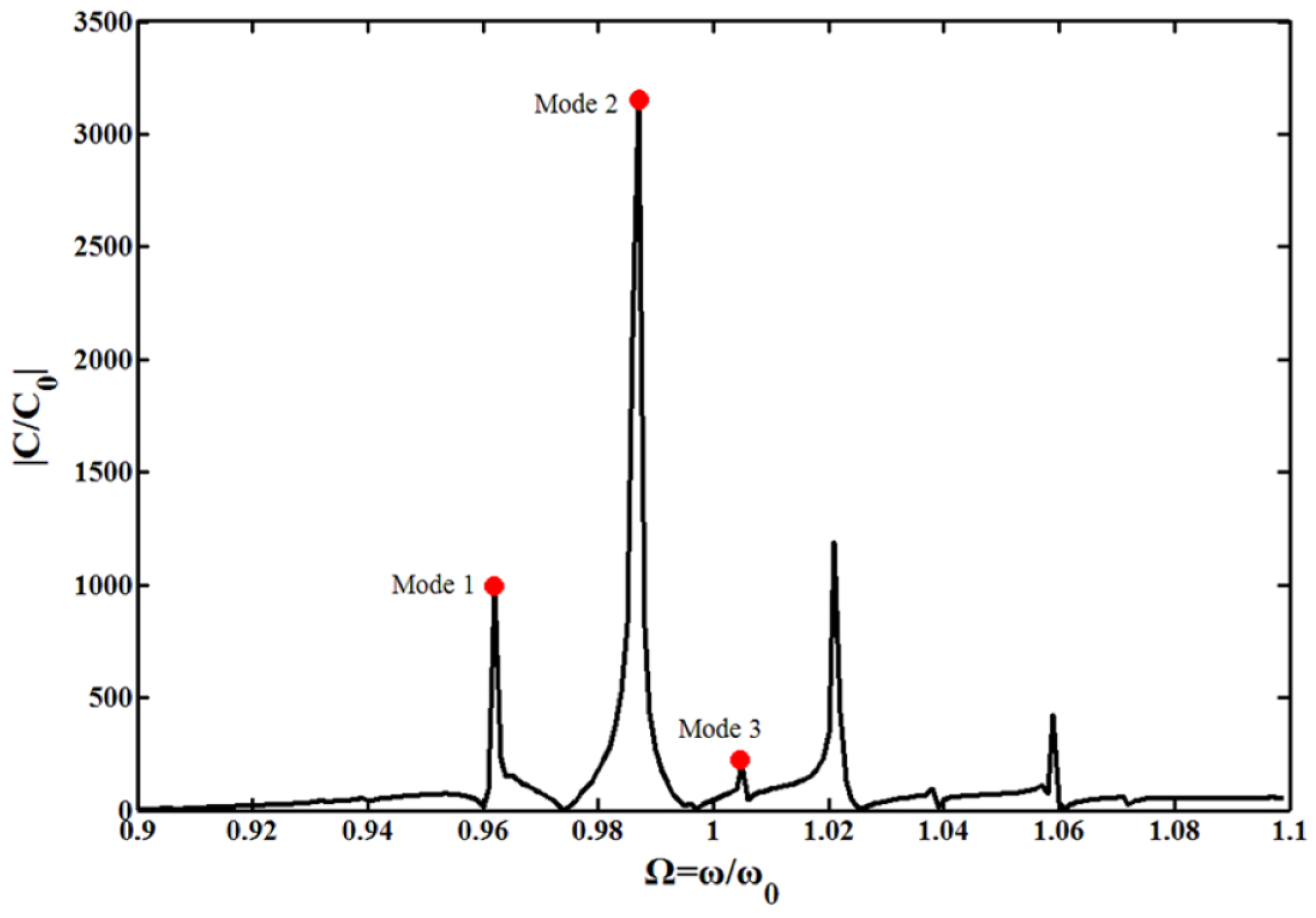
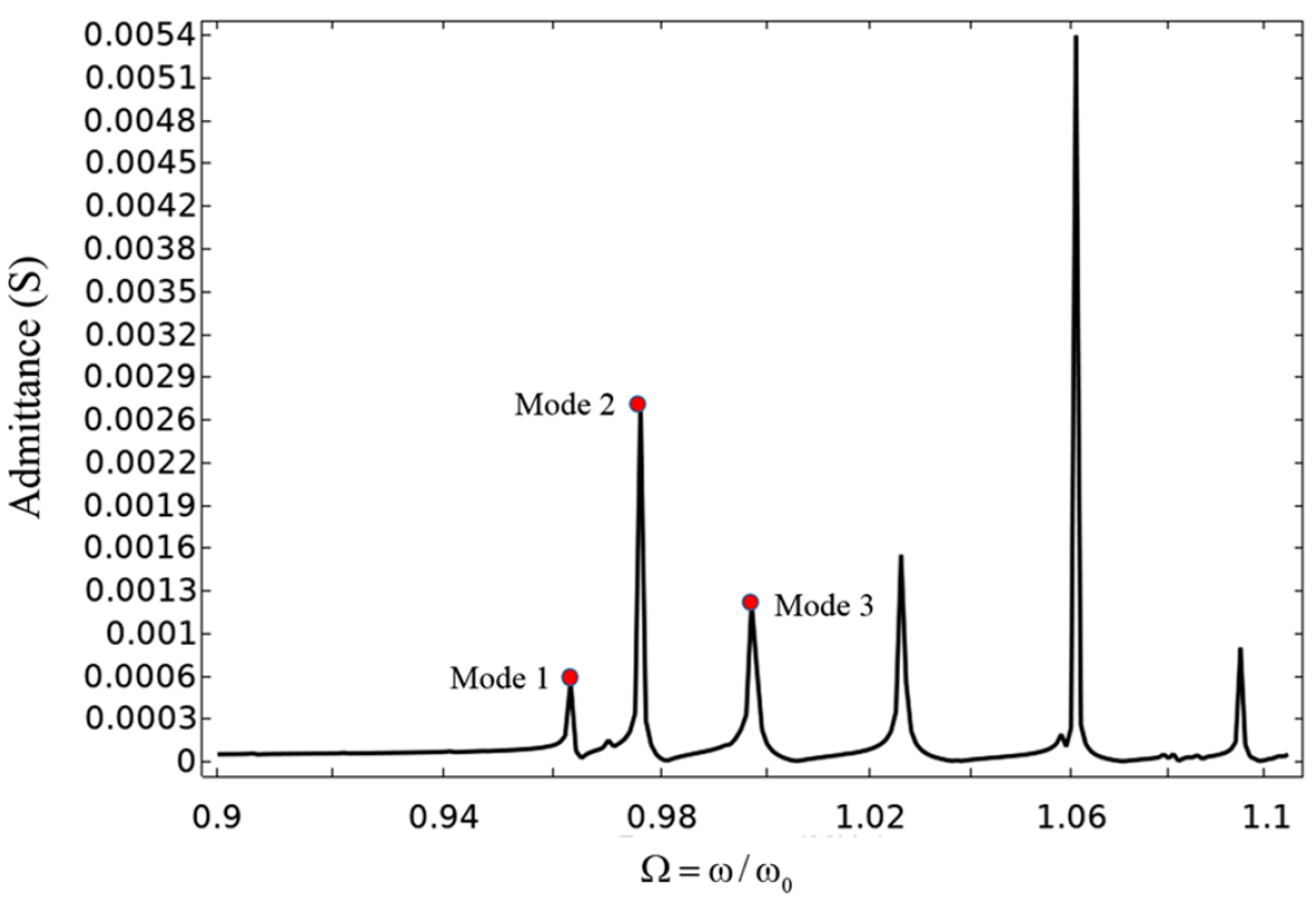
Figure 3 shows the curve of the resonator capacitance C versus the driving frequency. C is normalized by C 0 = 4 ε 11 h w / ( 2 c ) = 0.038 pF . ω 0 = ( π / 2 h ) c 66 / ρ = 10 MHz . Three fundamental resonance frequencies, including Modes 1, 2, and 3 in Figure 3 could be found, denoted by 0.962, 0.987, and 1.005 ω0, respectively.
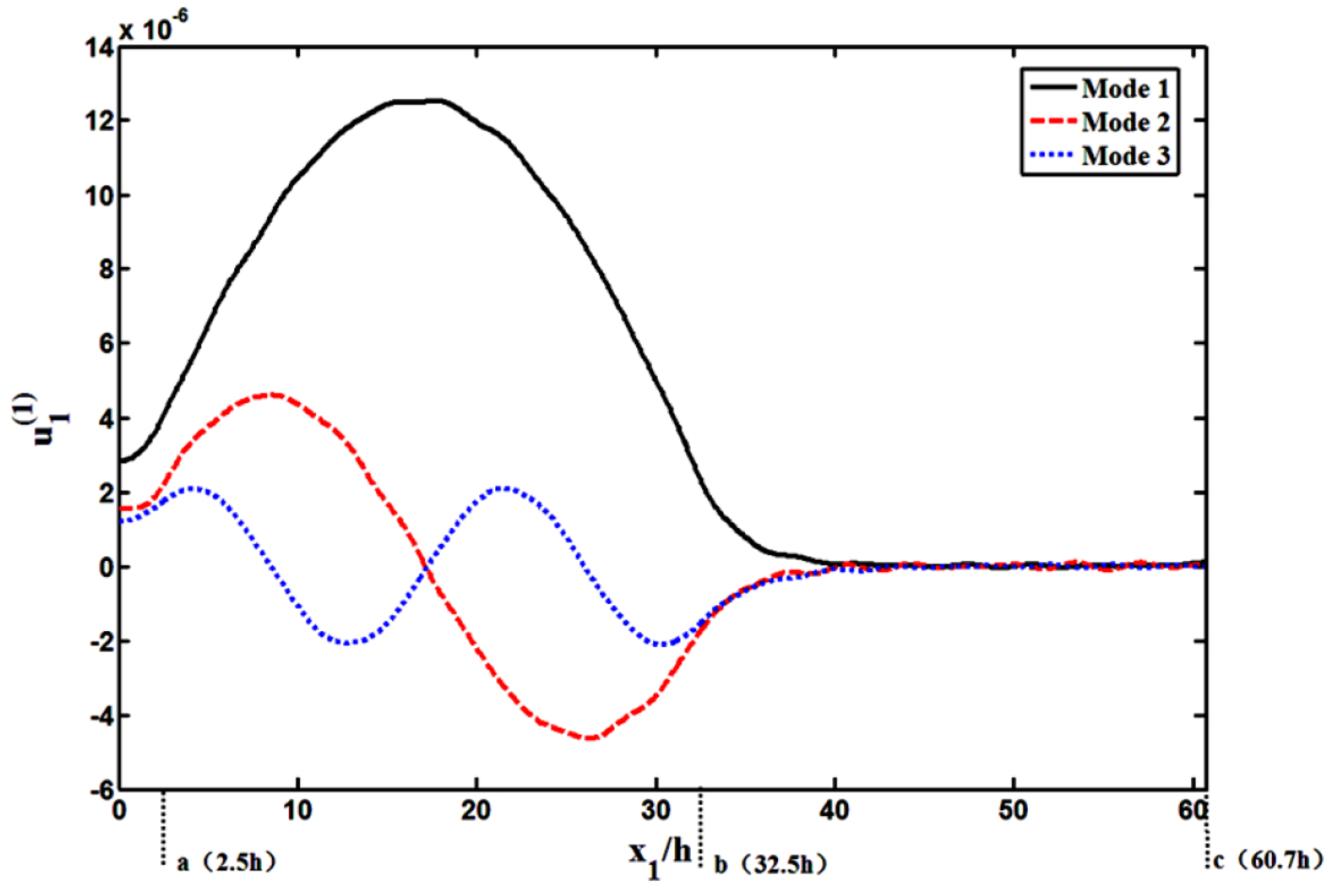
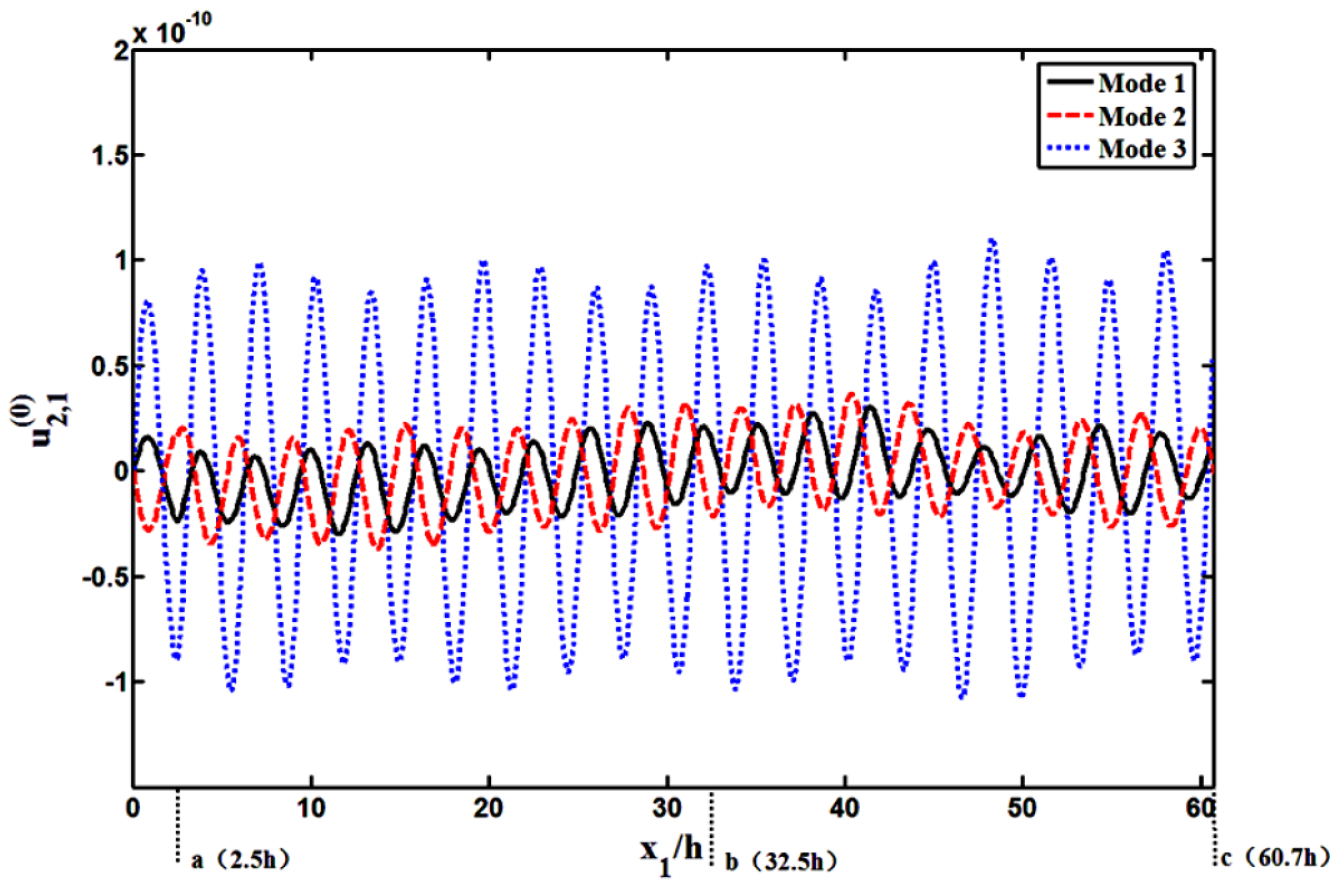
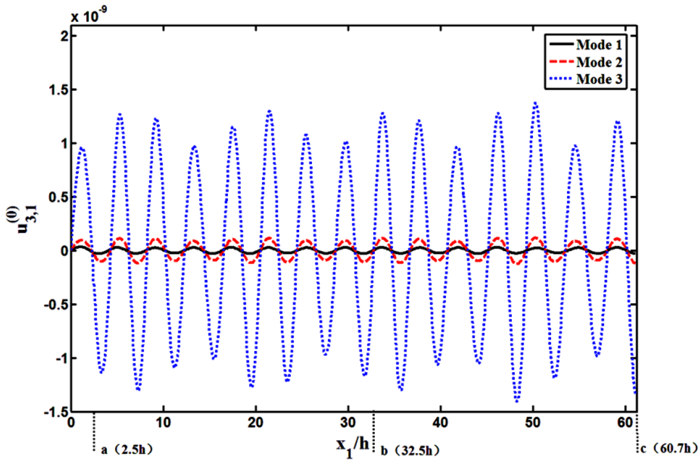
To evaluate the three fundamental resonances in the frequency domain of interest in Figure 3 accurately, the corresponding TSh strain distribution u 1 ( 1 ) ( x 1 ) , F strain distribution u 2 , 1 ( 0 ) ( x 1 ) and FS strain distribution u 3 , 1 ( 0 ) ( x 1 ) are plotted in Figure 4, Figure 5 and Figure 6, respectively. As shown in Figure 4, the TSh mode distribution for Mode 1 is considerable in the central gap area between the two electrodes and under the electrodes. Nevertheless, it reduces rapidly to zero around the plate edge. The above phenomenon is called energy trapping. In Figure 5 and Figure 6, it is shown that for Mode 1, the F and FS strains are both weak. Therefore, Mode 1 meets the resonator design requirements, namely, the operating mode is significant and the other modes coupled are weak. For Mode 2, the TSh strain has two valleys between the electrodes and under the electrodes area, as shown in Figure 4, which will cause additional shear strain to appear. Thus, this mode is undesirable for resonators. For Mode 3, there are four valleys for the TSh strain in Figure 4, and the F and FS strains are quite strong in Figure 5 and Figure 6; therefore, this mode is also not what we need.
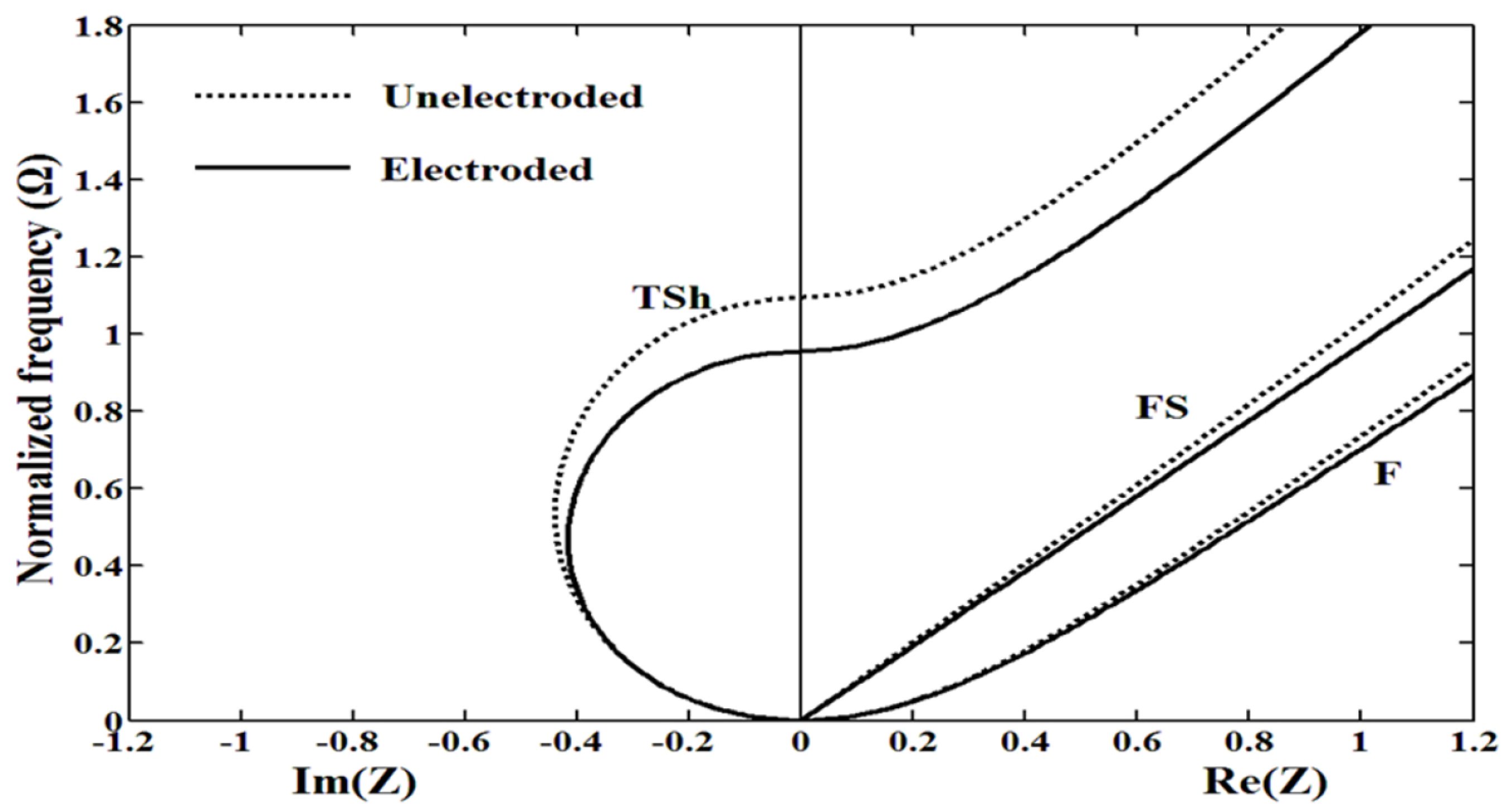
From the dispersion relationships shown in Figure 2, it is shown that when the wave number increases, the resonance frequency increases more slowly. Thus, although the differences in wave numbers of Modes 1, 2, and 3 shown in Figure 4 are large, the differences in the resonance frequencies of Modes 1, 2, and 3 shown in Figure 3 are small. It can be seen that from the dispersion curves (Figure 2), the wave numbers of the flexural and face-shear modes are obviously larger than that of the thickness-shear mode when the frequencies are the same. For the strain amplitudes, the vibration strength is closely related to the cut orientation of the crystal. The cut orientation in this paper is (yxl) 90°. In Ref [21], it was verified that the main mode of LiTaO3 plate with this cut orientation is the thickness-shear mode. Thus, compared with the thickness-shear mode, the flexural and face-shear modes have smaller strain distributions.
Further, a three-dimensional FEM analysis is carried out on the LiTaO3 LFE resonator operating with Mode 1 by the frequency domain calculation. The purpose of applying the FEM is to verify the reliability of the theoretical analysis method. Compared to the FEM calculation, the theoretical model can be used to explain the influence mechanism of the size parameters on the vibration properties of the device more conveniently. In addition, the calculation efficiency of the theoretical model is higher than that of FEM.
The admittance curves and the vibration mode shapes are plotted in Figure 7 and Figure 8, respectively. Figure 7 shows that the resonance frequency of the device is 0.9639 ω0. The theoretical frequency of Mode 1, shown in Figure 3, is 0.962 ω0. There is a 0.197% deviation between the FEM and the theoretical results of Mode 1. The deviation mainly attributes the differences between the 3D model of COMSOL and the 2D-approximate Mindlin plate theory. In addition, there emerge more spurious modes in the admittance curve of the device from the 3D FEM simulation, compared with the capacitance ratio curve obtained by the theoretical model. In Figure 8, it can be seen that the vibrations are concentrated in the electroded area. In the area near the edge of the plate, the vibration decays rapidly to almost zero. This means that the resonator has a good energy trapping at the resonant frequency of 0.9639 ω0.
The resonance frequencies of the resonators for varied electrode/plate mass ratio R, electrode gap a and the electrode width b are obtained. 
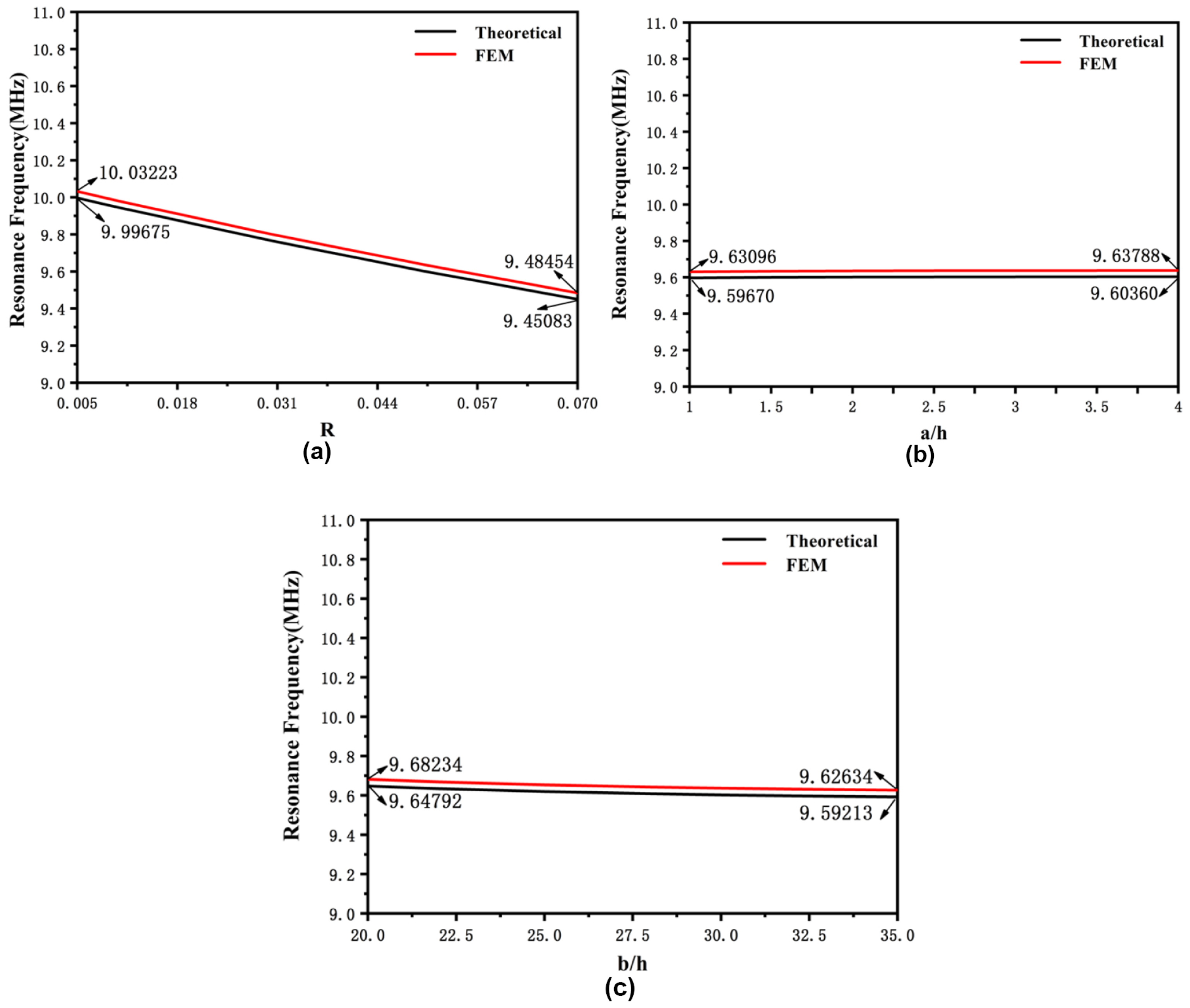
Figure 9a shows that the resonance frequency decreases approximately linearly as the electrode/plate mass ratio R varies from 0.005 to 0.07, while all other parameters are kept the same as those for Figure 3, Figure 4, Figure 5, Figure 6, Figure 7 and Figure 8. In Figure 9b, it is shown that the resonance frequency increases by 6.9 kHz as the electrode gap a varies from h to 4h, while keeping all other size factors the same as those for Figure 3, Figure 4, Figure 5, Figure 6, Figure 7 and Figure 8. As the electrode gap a increases, the two electrodes get farther apart, which leads to the mass effect being reduced and the resonance frequency increasing. In Figure 9c, for an increasing electrode width b, the corresponding resonance frequency decreases. This is because, as the electrode width b increases, the mass effect becomes more obvious. The theoretical trend is consistent with the FEM trend.
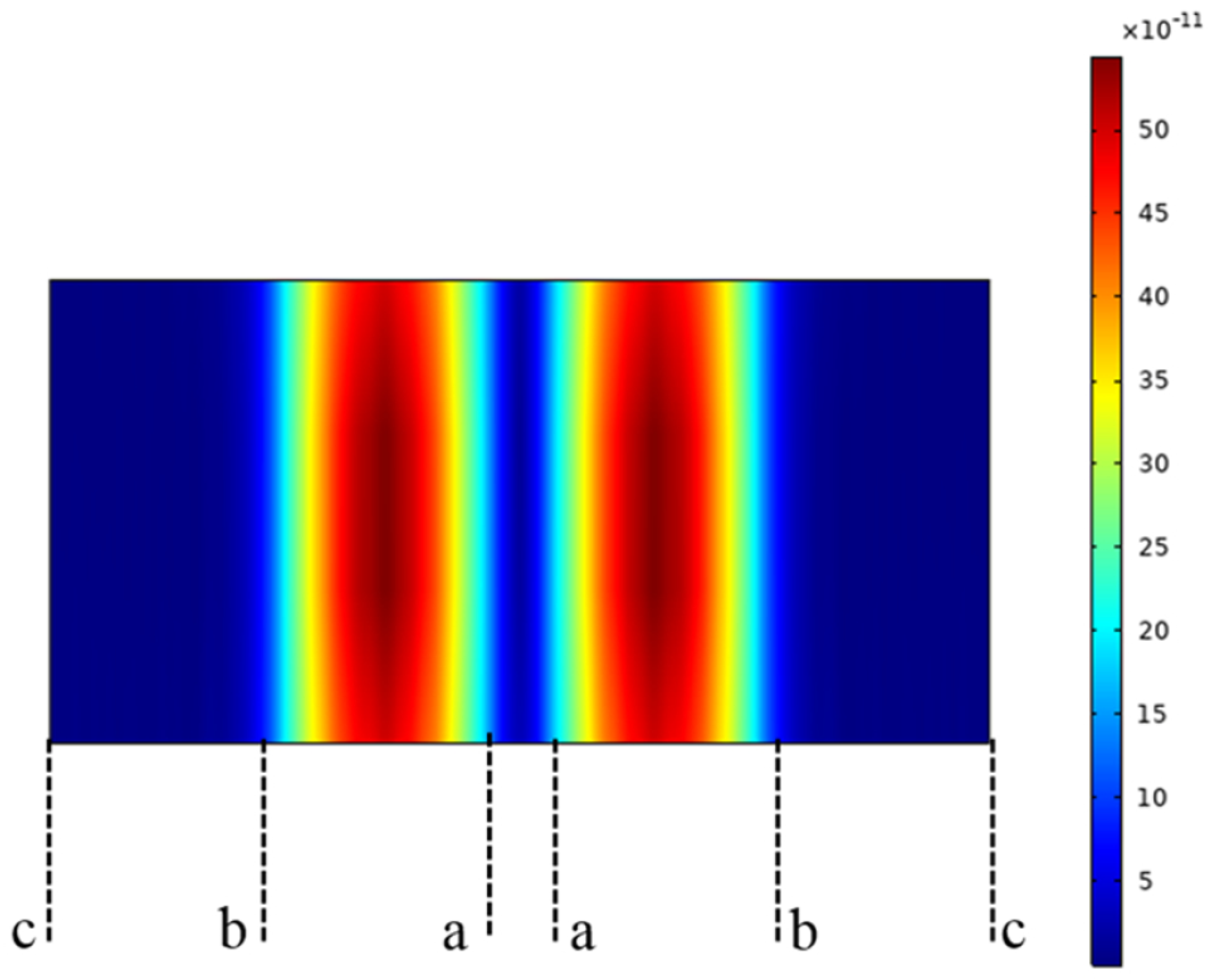
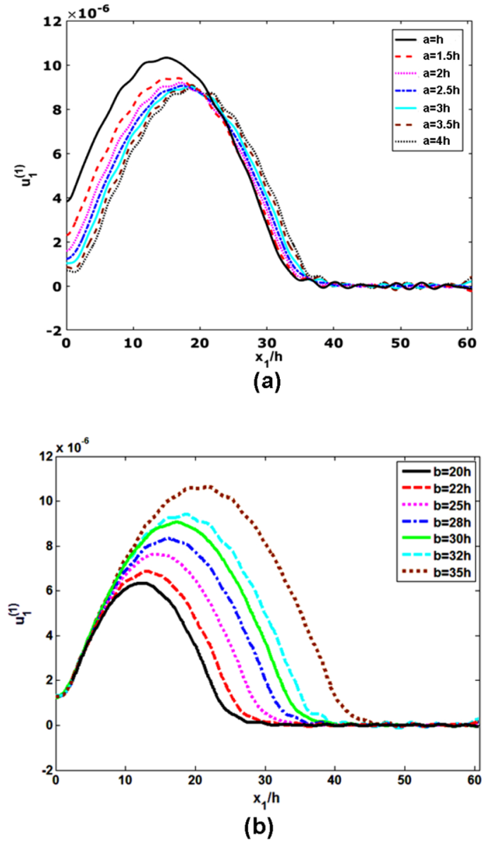
In addition, in order to reveal the influences of different size parameters on the vibration intensity and energy trapping of the resonator, the TSh strain distribution ( u 1 ( 1 ) ) for different gap values and electrode width values, obtained by using the theoretical model, is shown in Figure 10a,b, respectively. In Figure 10a, 2h = 0.1775 mm, b = 2.88 mm, c = 5.39 mm, R = 0.05, and w = 5.3 mm are fixed. In Figure 10b, 2h = 0.1775 mm, a = 2.22 mm, c = 5.39 mm, R = 0.05, and w = 5.3 mm are fixed.
It is shown in Figure 10a that, when the electrode gap a decreases, the vibration intensity of the device in the central area obviously increases, which can lead to a higher Q-factor and resonance stability. If the gap value a is small enough, the vibration strain in the area between the two electrodes will become too large and, thus, the energy trapping characteristic will become poor, which will decrease the frequency stability. Usually, to avoid a poor energy trapping, the vibration strain in the area between the two electrodes should be lower than one fifth of that of the peak. Therefore, on the premise of the above energy trapping requirement, it should reduce the gap value as far as possible to obtain a high Q-factor when selecting the electrode gap. In Figure 10b, as the electrode width b increases, the vibration intensity of the resonator increases, which can lead to a higher Q-factor. However, if the electrode width b is too large, the vibration strain around the plate edge will be obvious. The area around the plate edge is the mounting area, which is usually one tenth of the plate width. For the mounting area, the vibration strain needs to be close to zero, to reduce the impact of the mounting on the vibration properties of the device. Therefore, the selection criteria for the electrode width b of the resonator should be balanced between the Q-factor and the requisite mounting area with no vibration. Namely, on the premise of satisfying the mounting condition, it should increase the electrode width as far as possible to obtain a high Q-factor.

6. Conclusions

In this paper, the piezoelectric resonator based on a LiTaO3 single crystal stimulated via the lateral electric field is modeled and analyzed. The capacitance–frequency curve shows that there are several resonances around the main TSh frequency. The resonances are related to the TSh, FS and F modes. The TSh vibrations could be trapped in the area with the electrode. The influences of structural parameters such as the electrode/plate mass ratio, electrode gap and electrode width on the resonance frequency are studied by theoretical and FEM calculations. Both theoretical and FEM results show that the resonance frequency of the resonator increases with an increase in the electrode gap value or a decrease in the electrode width value. Additionally, the design criteria for the electrode gap and electrode width are given though analyzing the effects of those parameters on vibration strain distribution. Namely, when selecting the electrode gap, on the premise of the energy trapping requirement, it should reduce the gap value as far as possible to obtain a high Q-factor or good resonance stability. When selecting the electrode width, based on satisfying the mounting condition, it should increase the electrode width as far as possible to improve the resonance stability.

Author Contributions

H.S., T.M and H.Z. presented the idea and performed the theoretical analysis. L.Y. (Liang Yan), Y.Z. and H.S. accomplished the FEM analysis. Discussion about the results and the manuscript writing is contributed by H.S., T.M., H.Z., L.Y. (Liang Yan), Y.Z., M.W., B.H., J.W., J.D., L.Y. (Lili Yuan). All authors have read and agreed to the published version of the manuscript.

Funding

The current study was supported by the National Natural Science Foundation of China (Nos. 11772163, 11372146, 11702150, 11672142, 11672141, 11972354, 11772349), the Natural Science Foundation of Zhejiang Province (No. LY19A020003), and the special research funding from the Marine Biotechnology and Marine Engineering Discipline Group in Ningbo University.

Conflicts of Interest

The authors state that there is no conflict of interest.

References

  1. Latif, U.; Rohrer, A.; Lieberzeit, P.A.; Dickert, F.L. QCM gas phase detection with ceramic materials—VOCs and oil vapors. Anal. Bioanal. Chem. 2011, 400, 2457–2462. [Google Scholar] [CrossRef] [PubMed]
  2. Shen, D.Z.; Zhang, H.T.; Kang, Q.; Zhang, H.J.; Yuan, D.R. Oscillating frequency response of a langasite crystal microbalance in liquid phases. Sens. Actuators B. 2006, 119, 99–104. [Google Scholar] [CrossRef]
  3. Stevens, D.S.; Tiersten, H.F. An analysis of doubly rotated quartz resonators utilizing essentially thickness modes with transverse variation. J. Acoust. Soc. Am. 1986, 79, 1811–1826. [Google Scholar] [CrossRef]
  4. Hu, Y.T.; Yang, J.S.; Zeng, Y.; Jiang, Q.A. high-sensitivity, dual-plate, thickness-shear mode pressure sensor. IEEE Trans. Ultrason. Ferroelectr. Freq. Contr. 2006, 53, 2193–2197. [Google Scholar] [CrossRef] [PubMed]
  5. Wang, S.H.; Shen, C.Y.; Lin, Y.M.; Du, J.C. Piezoelectric sensor for sensitive determination of metal ions based on the phosphate-modified dendrimer. Smart Mater. Struct. 2016, 25, 085018. [Google Scholar] [CrossRef]
  6. Liu, N.; Yang, J.S.; Jin, F. Transient thickness-shear vibration of a piezoelectric plate of monoclinic crystals. Int. J. App. Electrom. 2012, 38, 27–37. [Google Scholar] [CrossRef]
  7. Qian, Z.H.; Kishimoto, K.; Yang, J.S. Propagation of thickness-twist wave in a piezoelectric ceramic plate in contact with viscous fluids. Acta Mech. 2010, 212, 263–270. [Google Scholar] [CrossRef]
  8. Ballato, A.; Hatch, E.R.; Mizan, M.; Lukaszek, T.J. Lateral Field Equivalent Networks and Piezocoupling Factors of Quartz Plates Driven in Simple Thickness Modes. IEEE Trans. Ultrason. Ferroelect. Freq. Contr. 1986, 33, 385–393. [Google Scholar] [CrossRef] [PubMed]
  9. Yang, J.S. The Mechanics of Piezoelectric Structures; World Scientific: Singapore, 2006. [Google Scholar]
  10. Liu, B.; Jiang, Q.; Hu, Y.T.; Yang, J.S. High-frequency vibrations of piezoelectric plates driven by lateral electric fields. Int. J. Eng. Sci. 2011, 49, 1435–1442. [Google Scholar] [CrossRef]
  11. Hu, Y.H.; French, L.A.; Radecsky, K.; Da Cunha, M.P.; Millard, P.; Vetelino, J.F. A lateral field excited liquid acoustic wave sensor. IEEE Trans. Ultrason. Ferroelectr. Freq. Contr. 2004, 51, 1373–1380. [Google Scholar] [CrossRef] [PubMed]
  12. Hempel, U.; Lucklum, R.; Hauptmann, P.; EerNisse, E.P.; Puccio, D.; Diaz, R.F.; Vives, A.A. Lateral field excited quartz crystal resonator sensors for determination of acoustic and electrical properties of liquids. In Proceedings of the 2008 IEEE Frequency Control Symposium, Aonolulu, HI, USA, 19–21 May 2008; pp. 705–710. [Google Scholar]
  13. Hu, Y.; Pinkham, W.; French, L.A., Jr.; Frankel, D.; Vetelino, J.F. Pesticide detection using a lateral field excited acoustic wave sensor. Sens. Actuators B 2005, 108, 910–916. [Google Scholar] [CrossRef]
  14. Hempel, U.; Lucklum, R.; Hauptmann, P.R. Lateral Field Excited Acoustic Wave Devices: A New Approach to Bio-Interface Sensing. In Proceedings of the 2007 IEEE Frequency Control Symposium, Geneva, Switzerland, 1 October 2007; pp. 426–430. [Google Scholar]
  15. Martin, S.J.; Granstaff, V.E.; Frye, G.C. Characterization of a quartz crystal microbalance with simultaneous mass and liquid loading. Anal. Chem. 1991, 63, 2273–2281. [Google Scholar] [CrossRef]
  16. Vetelino, J.F.; Reghu, A. Introduction to Sensors; CRS Press: Boca Raton, FL, USA, 2010. [Google Scholar]
  17. Warner, A.W.; Onoe, M.; Coquin, G.A. Determination of Elastic and Piezoelectric Constants for Crystals in Class (3m). J. Acoust. Soc. Am. 1967, 42, 1223–1231. [Google Scholar] [CrossRef]
  18. Liu, B.; Jiang, Q.; Xie, H.M.; Yang, J.S. Energy trapping in high-frequency vibrations of piezoelectric plates with partial mass layers under lateral electric field excitation. Ultrasonics 2010, 51, 376–381. [Google Scholar] [CrossRef] [PubMed]
  19. Wang, W.Y.; Zhang, C.; Zhang, Z.T.; Liu, Y.; Feng, G.P. Three operation modes of lateral-field-excited piezoelectric devices. Appl. Phys. Lett. 2008, 93, 242906. [Google Scholar] [CrossRef]
  20. Khan, A.; Ballato, A. Piezoelectric coupling factor calculations for plates of langatate driven in simple thickness modes by lateral-field-excitation. IEEE Trans. Ultrason. Ferroelectr. Freq. Control. 2002, 49, 922–928. [Google Scholar] [CrossRef] [PubMed]
  21. Ma, T.F.; Zhang, C.; Zhang, Z.T.; Wang, W.Y.; Feng, G.P. Investigation of lateral-field-excitation on LiTaO3 Single Crystal. In Proceedings of the 2010 IEEE International Frequency Control Symposium, Newport Beach, CA, USA, 1–4 June 2010; pp. 489–492. [Google Scholar]
  22. Mindlin, D.; Spencer, W.J. Anharmonic, thickness-twist overtones of thickness-shear and flexural vibrations of rectangular, AT-cut quartz plates. J. Acoust. Soc. Am. 1967, 42, 1268–1277. [Google Scholar] [CrossRef]
  23. Auld, B.A. Acoustic Fields and Waves in Solids; Wiley: New York, NY, USA, 1973; Volume I. [Google Scholar]
Figure 1. A LiTaO3 crystal plate with lateral field excitation.
Crystals 10 00525 g001
Figure 2. Dispersion relationships of (yxl) 90° LiTaO3 plates for lateral field excitation.
Crystals 10 00525 g002
Figure 3. Normalized capacitance with respect to diving frequency showing resonance modes.
Crystals 10 00525 g003
Figure 4. Thickness-shear (TSh) strain distribution ( u 1 ( 1 ) ) near resonance.
Crystals 10 00525 g004
Figure 5. Flexural (F) strain distribution ( u 2 , 1 ( 0 ) ) near resonance.
Crystals 10 00525 g005
Figure 6. Face-shear (FS) strain distribution ( u 3 , 1 ( 0 ) ) near resonance.
Crystals 10 00525 g006
Figure 7. The admittance curve of the lateral field excitation (LFE) resonator from COMSOL.
Crystals 10 00525 g007
Figure 8. The vibration mode shape of the LFE resonator from COMSOL.
Crystals 10 00525 g008
Figure 9. Resonance frequencies of resonators for varied parameters: (a) electrode/plate mass ratio R; (b) electrode gap a; (c) electrode width b.
Crystals 10 00525 g009
Figure 10. Effects of the size parameters on the TSh strain distribution u 1 ( 1 ) : (a) electrode gap a; (b) electrode width b.
Crystals 10 00525 g010

