Integral Characteristic of Complex Catalytic Reaction Accompanied by Deactivation

Abstract

New theoretical relationships for a complex catalytic reaction accompanied by deactivation are obtained, using as an example the two-step catalytic mechanism (Temkin–Boudart mechanism) with irreversible reactions and irreversible deactivation. In the domain of small concentrations, $A_{\lim }=N_S\frac{k_1{C}_A}{k_d},$ where $A_{\lim }$ is the limit of the integral consumption of the gas substance, $N_S$ is the number of active sites per unit of catalyst surface; $k_1$ and $k_d$, are kinetic coefficients which relate to two reactions which compete for the free active site Z. $C_A$ is the gas concentration. One reaction belongs to the catalytic cycle. The other reaction with kinetic coefficient $k_d$ is irreversible deactivation. The catalyst lifetime, ${\tau }_{\mathrm{cat}}=\frac{1}{C_Z^{\prime }}\frac{1}{k_d}$, where $C_Z^{\prime }$ is the dimensionless steady-state concentration of free active sites. The main conclusion was formulated as follows: the catalyst lifetime can be enhanced by decreasing the steady-state (quasi-steady-state) concentration of free active sites. In some domains of parameters, it can also be achieved by increasing the steady-state (quasi-steady-state) reaction rate of the fresh catalyst. We can express this conclusion as follows: under some conditions, an elevated fresh catalyst activity protects the catalyst from deactivation. These theoretical results are illustrated with the use of computer simulations.

1. Introduction

Catalyst deactivation is a complex, non-steady-state process governed by a variety of phenomena that are influenced by many physicochemical factors.

In the literature, different types of kinetic models of catalytic reactions with deactivation were proposed, i.e., phenomenological models, detailed kinetic models, and semi-phenomenological models.

1.1. Phenomenological Models

In phenomenological models of ‘gas-solid’ catalytic reactions, the main characteristic of the catalytic process, the reaction rate (r), is presented as a function of the concentrations of the reactants ($C=C_1,C_2,\dots$), the temperature (T), and catalyst activity (a),

$$r=f(C,T,a).$$

(1)

The catalyst activity a is considered a function of the reaction conditions, here C and T, and its change can be called ‘catalyst deactivation’.

The first kinetic phenomenological model was formulated by Szépe and Levenspiel [1].

$$\begin{array}{cc}\hfill r\left(t\right)=& R_{0}a\left(t\right)\hfill \end{array}$$

(2)

$$\begin{array}{cc}\hfill \frac{da}{dt}=& f(C,T)a^d\hfill \end{array}$$

(3)

where $R_0$ is the reaction rate over the non-deactivated (‘fresh’) catalyst and d is an empirical parameter.

These models are called separable because the reaction kinetics and deactivation kinetics are assumed to be separate, see papers by Corella et al. [2,3] as well.

Froment and Bischoff [4,5] introduced the activity parameter

$$\Phi =\frac{k}{k_0}$$

(4)

(that is the ratio of the reaction rate constants of the deactivated k and of the ‘fresh’ catalyst $k_0$) and considered it as a function of coke concentration. They proposed three functions:

$$\begin{array}{cc}\hfill \mathrm{linear}:& {\Phi }_1=1-\gamma C_c,\hfill \end{array}$$

(5)

$$\begin{array}{cc}\hfill \mathrm{exponential}:& {\Phi }_2=exp\left(-\gamma C_c\right),\hfill \end{array}$$

(6)

$$\begin{array}{cc}\hfill \mathrm{hyperbolic}:& {\Phi }_3=\frac{1}{1+\gamma C_c}.\hfill \end{array}$$

(7)

Later, these relationships were used in many studies to describe the coking and deactivation of the catalysts in the processes of dehydrogenation, cracking, etc. In these processes, the activity changes rapidly, Therefore, in this case the quasi-steady-state assumption does not make the task easier.

Beeckman, Marin, and Froment [6,7] developed the probabilistic model of catalyst coking that implies coke deposition on the active and coked surface.

In this model, the catalyst activity is the product of two probabilities:

$$a=PS,$$

(8)

where S is the probability that an active site is not covered with coke; P is the probability that an active site is not locked as a result of pore blockage.

In reactors with the moving and fluidized bed, the coke concentration measurement becomes as accessible as the reactant concentration measurement (i.e., conversion and activity calculation). Therefore, it becomes important to express activity via coke concentration.

Such dependencies were derived by Ostrovskii based on the multilayer mechanism of coke formations.

Two equations were obtained, corresponding to infinite coke formation and a finite number of layers:

$$\begin{array}{cc}\hfill \frac{C_c}{C_m}=& \left(1-\phi \right)\left(1-a\right)-\phi lna,\hfill \end{array}$$

(9)

$$\begin{array}{cc}\hfill \frac{C_c}{C_m}=& N-a-(N-1)a^{\phi }.\hfill \end{array}$$

(10)

where $C_m$ is the monolayer coke concentration; $\phi$ is the ratio of rate constants of poly- and monolayer coking; N is the number of coke layers.

1.2. Detailed Kinetic Models

In detailed models (micro-kinetic or mechanistic models), the model is based on the mechanism, i.e., the set of steps that include reactants and products of the overall reactions as well as catalytic intermediates.

A detailed kinetic model was presented in [8] with a description of two different periods of irreversible deactivation. However, even presently, 50 years later, the number of papers with detailed kinetic models of catalyst deactivation is limited, since the information on the evolution of the surface composition is in short supply.

1.3. Semi-Phenomenological Models

In the catalytic literature, many models have been presented combining phenomenology with some mechanistic considerations of deactivation, e.g., power-law kinetic dependencies and Langmuir–Hinshelwood–Hougen–Watson relationships based on the concept of adsorption equilibrium, see Butt [9] and Bartholomew [10]. In our paper [11], such models are called semi-phenomenological.

In 1989, Ostrovskii and Yablonskii [12] proposed the semi-phenomenological model of single-route catalytic reactions assuming two types of catalyst deactivation, i.e., reversible and irreversible (‘aging’). In deriving this model, the known principle of quasi-steady-state (QSS) concentrations was used to obtain the concentration of the catalytic intermediate, which deactivates during the process. This concentration was presented as a function of the QSS reaction rate and other kinetic parameters. Later, Ostrovskii developed this approach further in the monograph [13] and paper [14].

In our paper [11], the same approach was presented for the rigorous derivation of the kinetic equation of the n-step single-route catalytic reaction accompanied by two processes of catalytic deactivation, one reversible and the other irreversible. Here the term “reversible deactivation” refers to the fact that the deactivation step includes two reactions, a forward, and a reverse one.

This catalytic process was described by the three-building-block scheme (Figure 1). There we considered a linear mechanism for the catalytic cycle, i.e., only one ‘molecule’ of the catalytic intermediate, including the active center, participates in each reaction.

Applying the new, more convenient form of the rate equation for the single-route catalytic reaction with the linear mechanism [15], resulted in the three-factor kinetic equation of deactivation [11] for this complex process.

$$\begin{array}{cc}\hfill R\left(t\right)=& N_S^0{R}_{\mathrm{fresh}}{\psi }_{r,d}{\psi }_{i,d},\hfill \end{array}$$

(11)

$$\begin{array}{cc}\hfill {\psi }_{r,d}=& \underset{\mathrm{reversible\; deactivation\; factor}}{\underbrace{\frac{1+\alpha K_d{R}_{\mathrm{fresh}}exp\left(-\left(1+\alpha K_d{R}_{\mathrm{fresh}}\right)k_{r,d}t\right)}{1+\alpha K_d{R}_{\mathrm{fresh}}}}},\hfill \end{array}$$

(12)

$$\begin{array}{cc}\hfill {\psi }_{i,d}=& \underset{\mathrm{irreversible\; deactivation\; factor}}{\underbrace{exp\left(-\frac{\alpha K_d{R}_{\mathrm{fresh}}}{1+\alpha K_d{R}_{\mathrm{fresh}}}{k}_{i}t\right)}},\hfill \end{array}$$

(13)

where $N_S^0$ is the initial number of active sites per unit of catalyst surface; $R_{\mathrm{fresh}}$ is the ‘fresh’ rate of the main catalyst cycle; $\alpha R_{\mathrm{fresh}}=C_{Z,\mathrm{fresh}}^{\prime }$ is the ‘fresh’ concentration of free catalyst active site Z and where $\alpha$ is a special parameter described in [11]; $K_d$ is the equilibrium constant of the reversible deactivation reaction; and $k_i$ is the rate constant of the irreversible deactivation reaction.

This deactivation equation with some simplifications will be used in this paper for different purposes. As mentioned, the quasi-steady-state hypothesis (QSSH) was applied as a tool for the derivation of this deactivation equation. The status of the QSSH in our problems should be discussed in more detail.

This model is an advantageous simplification of the mechanistic model. It is based on the idea of a cyclic catalytic mechanism, and its constituents are the concept of active sites and assumptions on fast and slow parameters considering the quasi-steady-state principle. In comparison with the recent all-component-model, e.g., Cordero-Lanzac et al. [16], and detailed multi-step and multi-route models [17,18] see also Cordero-Lanzac’s dissertation, the semi-phenomenological model used in this paper has obvious advantages:

• the number of parameters is much smaller;
• this model allows the derivation of interesting analytical results, as will be demonstrated in this paper;
• potentially, this simpler model can be useful for the design of catalytic reactors with deactivation and optimization of industrial regimes.

One of the main ideas of chemical kinetics is a hierarchy, i.e., the time scale separation, based on the large difference in magnitude of the parameters of the kinetic model. This hierarchy determines a variety of different cases and regimes, e.g., quasi-equilibrium (QE), quasi-steady-state (QSS), limiting step (LS), assumptions on most abundant reactive intermediates (mari) or surface intermediates (masi), and, finally, lumping.

The quasi-steady-state (QSS) approximation is the central one among all these simplifications. The QSS-principle regarding kinetic intermediates of a complex chemical reaction is typically attributed to Bodenstein [19] and sometimes to Chapman [20,21] as well, see the historical information [22,23].

It was based on the idea of fast intermediates, i.e., the kinetic parameters related to some intermediates are much larger than the kinetic parameters related to stable molecules.

In the pioneering paper by Michaelis–Menten [24], two hierarchies were considered:

• a large difference in kinetic parameters
• a large difference between the total amounts of main reactants and the total amount of intermediates. For the ‘gas-solid’ catalytic reaction, the latter corresponds to the case when the total number of active catalytic centers is much smaller than the total number of reactant and product molecules, see [22] (Chapter 3).

Gorban and Shahzad [25] theoretically revisited and generalized the Michaelis–Menten approach. It was shown that, rigorously speaking, the Michaelis–Menten kinetics, as we refer to it presently, should be attributed to Briggs and Haldane [26].

In accordance with the QSS method, the derivatives of the chemical intermediates are replaced by ‘zeros’, and the corresponding differential equations transform to algebraic ones.

This ‘trick’ became an extremely popular tool in the theoretical study of complex chemical reactions, both homogeneous and heterogeneous.

However, for a period of 50-plus years after the time of Bodenstein and Michaelis–Menten, the mathematical status of the QSS method was very unclear, there was no understanding of why the derivatives of ‘fast’ intermediates are replaced by zero. Only starting from the 1950s, a rigorous mathematical concept for QSS was created based on the theory of singularly perturbed ordinary differential equations (ODEs). This theory was developed by Tikhonov and his colleagues [27,28,29,30], and the central point of this theory was the concept of a so-called ‘small parameter’.

In 1955 Sayasov and Vasil’eva published the first pioneering paper [28] on the mathematical status of the QSS using a radical gas chain reaction with fast intermediates as an example. The small parameter was chosen as the ratio of kinetic parameters. A similar point of view was expressed in 1963 by Bowen, Acrivos, and Oppenheim [31].

In 1963, Heineken, Tsuchiya, and Aris (HTA) published a paper [32] on the mathematical status of the QSS for the Michaelis–Menten two-step mechanism. The small parameter used by HTA was the ratio of two numbers, the number of enzyme active sites and the number of substrate molecules. A similar small parameter, i.e., the ratio of the total amount of surface intermediates, mole, to the total amount of reacting components, mole, was used in monographs [22,23] for obtaining general results in catalytic kinetics (see also the early monograph [33]).

The general methodology in studying hierarchical kinetics, see “Asymptotology” by Gorban et al., [34,35,36] as well.

2. Goal of the Paper: General Problems and Specific Problems of This Paper

The goal of this paper is to present the integral characteristic A ($\mathrm{mol}{\mathrm{cm}}_{\mathrm{cat}}^{-2}$) of complex ‘gas-solid’ catalytic reactions accompanied by deactivation, i.e.,

$$A={\int }_0^{\tau }R\left(t\right)dt,$$

(14)

where $R\left(t\right)$ is the consumption rate of the gas reactant, or the rate of release of the gas product. It will be presented for some regimes as an analytical expression and will be illustrated using computational results.

Our goal will also be to estimate the catalyst lifetime by relating the value of A to the value of the quasi-steady-state (QSS) rate of the ‘fresh’ (non-deactivated) catalyst.

Our model of a complex catalytic reaction accompanied by deactivation includes two small parameters

• the small parameter which is caused by the difference between the number of catalyst active sites and the number of gaseous molecules (“the first small parameter”)
• the small parameter caused by the difference between the deactivation parameters and kinetic coefficients of the main catalytic cycle (“the second small parameter”)

In this paper, we are going to start the systematic application of our three-factor kinetic equation proposed in [11] to different problems of catalytic kinetics. The program of our studies will include different cases and scenarios. It is reasonable to expect that the results of our studies will depend on the type of the kinetic device and its kinetic model, on the analyzed chemical mechanisms and corresponding models, and the conditions of the process reversibility, i.e., whether deactivation is reversible or irreversible, whether the chemical catalytic cycle is reversible or irreversible etc.

Generally, we are planning to analyze the following cases:

• Kinetic models of the batch reactor (BR) and continuously stirred tank reactor (CSTR).
• Kinetic models of typical heterogeneous catalytic mechanisms:

  (a)

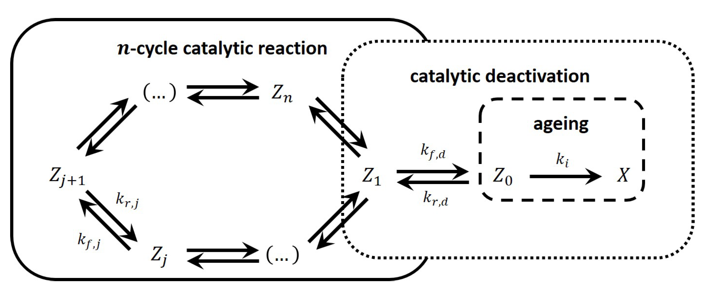
  The n-step single-route complex catalytic reaction with a linear mechanism.

  (b)

  The two-step catalytic mechanism (Temkin–Boudart mechanism) as a basic mechanism of theoretical chemical kinetics of heterogeneous catalysis [37,38,39].

• Models with reversible and irreversible steps in the catalytic cycle.
• Models with reversible and irreversible deactivation process.

In this paper, we will study the kinetic behavior of a batch reactor in which catalytic reactions are accompanied by deactivation. As an example the simplest two-step catalytic mechanism (Temkin–Boudart mechanism) is chosen with irreversible deactivation. It is the simplest mechanism of the ones mentioned above.

Different scenarios of the transient interplay between the main cycle relaxation and deactivation dynamics will be described, and different temporal and parametric domains will be distinguished:

• The initial non-steady-state kinetic regime caused by the intrinsic catalytic cycle.
• The quasi-steady-state regime regarding the catalytic intermediates with insignificant deactivation (’no deactivation’ regime). This regime is caused by the difference between the number of catalyst active sites and the number of gaseous molecules (“the first small parameter”).
• The quasi-steady-state regime regarding the intermediates in which the deactivation process is significant. Within this domain, the total number of active sites is decreased, and the quasi-steady-state regime becomes more pronounced.

Under concrete values of parameters, some domains can be negligible. Different questions will be answered:

• In which domain will the catalyst composition be nearly constant, i.e., despite the change in the number of active sites the relative concentrations of catalytic intermediates are remaining approximately the same?
• How to analyze the long-term behavior of the catalytic system with deactivation based on its integral characteristic?
• What is the best strategy for the increase of catalytic efficiency based on the kinetic description?

3. Theoretical Analysis

Our strategy is to first analyze the full model, i.e., the two-step irreversible catalytic cycle with irreversible deactivation, and then to analyze the three reduced models, two of which have “no” deactivation and are known in the literature, i.e.,

• Only the main catalytic cycle model; the non-steady-state case.
• Only the main catalytic cycle model; the quasi-steady-state case.

In our opinion, it is necessary to study these models to build a strong foundation and systematic framework on which to continue the analysis of more complex cases related to deactivation. We expect these simple models can be used as asymptotics for the more complex ones. This content will also help us to understand the final results for both the mathematical and chemical engineering communities.

3.1. The Full Model of the Two-Step Irreversible Catalytic Cycle with Irreversible Deactivation

We use the two-step catalytic mechanism of an isomerization reaction with irreversible steps,

$$\begin{gathered} \mathrm{A}+\mathrm{Z}\stackrel{k1}{\to }\mathrm{AZ} \\ \mathrm{and}\mathrm{AZ}\stackrel{k2}{\to }\mathrm{B}+\mathrm{Z} \end{gathered}$$

accompanied by a (possible) deactivation step,

$$\mathrm{Z}\stackrel{kd}{\to }\mathrm{X}.$$

The rate equations corresponding to these reactions are,

$$\begin{array}{cc}\hfill r_1=& k_1{C}_A{C}_Z,\hfill \end{array}$$

(15)

$$\begin{array}{cc}\hfill r_2=& k_2{C}_{AZ},\hfill \end{array}$$

(16)

$$\begin{array}{cc}\hfill \mathrm{and}{r}_d=& k_d{C}_Z,\hfill \end{array}$$

(17)

where $r_1$, $r_2$ and $r_d$ are rate equations in $\mathrm{mol}{\mathrm{cm}}_{\mathrm{cat}}^{-2}{\mathrm{s}}^{-1}$; $k_1$ is a reaction rate constant in ${\mathrm{cm}}_{\mathrm{gas}}^3{\mathrm{mol}}^{-1}{\mathrm{s}}^{-1}$; $k_2$ and $k_d$ are reaction rate constants in ${\mathrm{s}}^{-1}$; $C_A$ is the concentration of gas reactant A in mol ${\mathrm{cm}}_{\mathrm{gas}}^{-3}$; and $C_Z$ and $C_{AZ}$ are concentrations of active catalyst sites, also referred to as catalyst intermediates, in mol ${\mathrm{cm}}_{\mathrm{cat}}^{-2}$.

The kinetic equations for the gas reactant and product are,

$$\begin{array}{cc}\hfill \frac{d{C}_A}{dt}& =-\frac{S_{\mathrm{cat}}}{V_{\mathrm{gas}}}{r}_1,\hfill \\ & =-\frac{S_{\mathrm{cat}}}{V_{\mathrm{gas}}}{k}_1{C}_A(N_S-C_{AZ}),\hfill \end{array}$$

(18)

$$\begin{array}{cc}\hfill C_B=& N_V-C_A-\frac{S_{\mathrm{cat}}}{V_{\mathrm{gas}}}{C}_{AZ},\hfill \end{array}$$

(19)

where $C_B$ is the concentration of the gas product and $\frac{S_{\mathrm{cat}}}{V_{\mathrm{gas}}}$ is a factor consisting of ratio of the catalyst surface area $S_{\mathrm{cat}}$ (${\mathrm{cm}}_{\mathrm{cat}}^2$) to the gas volume (${\mathrm{cm}}_{\mathrm{cat}}^3$). Equation (19) is derived from the law of mass conservation for element A where $N_V$ is the total concentration of gas (mol ${\mathrm{cm}}_{\mathrm{cat}}^{-3}$).

The kinetic equations for the catalytic intermediates are,

$$\begin{array}{cc}\hfill \frac{d{C}_{AZ}}{dt}& =r_1-r_2,\hfill \\ & =k_1{C}_A(N_S-C_{AZ})-k_2{C}_{AZ},\hfill \end{array}$$

(20)

$$\begin{array}{cc}\hfill \frac{d{N}_S}{dt}=& -r_d,\hfill \\ \hfill =& k_d(N_S-C_{AZ}),\hfill \end{array}$$

(21)

$$\begin{array}{cc}\hfill C_Z=& N_S-C_{AZ},\hfill \end{array}$$

(22)

where $N_S$ is the total concentration of active catalyst sites in $\mathrm{mol}{\mathrm{cm}}_{\mathrm{cat}}^{-3}$. Equation (22) is derived from the law of mass conservation for the catalyst sites.

Equations (18)–(22) represent the dimensional system of equations for the full model. There are three differential equations, two non-linear (18), (20) and one linear (21), and two linear algebraic Equations (19) and (22).

In our analysis, we wish to differentiate between slow and fast behavior. To do this, we must first identify a small parameter. In some cases, one small parameter is enough. However, we will highlight two different small parameters for this specific work.

The first small parameter, ${\epsilon }_1$, is defined as the ratio of the number of catalyst sites to the number of gas molecules. At time zero, the number of catalyst sites is equal to the number of active catalyst sites. If there is deactivation, this equality will not hold anymore. This is why we use the initial (‘fresh’) number of active sites in our definition.

 Small Parameter 1. 

The ratio of the total number of ‘fresh’ active sites to the total number of gas molecules,

$${\epsilon }_1=\frac{S_{\mathrm{cat}}{N}_S^0}{V_{\mathrm{gas}}{N}_V}.$$

The parameters $S_{\mathrm{cat}}$, $V_{\mathrm{gas}}$, $N_S^0$ and $N_V$ are the catalyst surface (${\mathrm{cm}}_{\mathrm{cat}}^2$), gas volume (${\mathrm{cm}}_{\mathrm{cat}}^3$), the ‘fresh’ concentration of active sites, i.e., the concentration of active sites ($\mathrm{mol}{\mathrm{cm}}_{\mathrm{cat}}^{-2}$ ) at time zero, $N_S^0=N_S\left(0\right)$ and the total concentration of gas ($\mathrm{mol}{\mathrm{cm}}_{\mathrm{cat}}^{-3}$), respectively.

The second small parameter, ${\epsilon }_2$, is defined as the ratio of the deactivation parameter to a kinetic rate coefficient of the main catalytic cycle. The deactivation rate constant $k_d$ is assumed to be much smaller than the rate constants of the catalytic cycle $k_1{N}_V$ and $k_2$, i.e., $k_d\ll k_1{N}_V,k_2$. Our second small parameter can be interpreted as a dimensionless deactivation rate constant. We achieve this by either scaling with respect to $k_1{N}_V$ or $k_2$. We chose $k_1{N}_V$ here because the term reappears in several of the system equations.

 Small Parameter 2. 

The dimensionless deactivation rate constant,

$${\epsilon }_2=\frac{k_d}{k_1{N}_V}.$$

The parameters $k_d$, $k_1$ and $N_V$ are the deactivation rate constant (${\mathrm{s}}^{-1}$), the reaction rate constant of reaction 1 (${\mathrm{cm}}_{\mathrm{gas}}^3{\mathrm{mol}}^{-1}{\mathrm{s}}^{-1}$) and the total concentration of gas ($\mathrm{mol}{\mathrm{cm}}_{\mathrm{gas}}^{-3}$), respectively.

Implementing the small parameter into the kinetic equations for the reactant, product, and catalytic intermediates, we rewrite the equations for the full system (18)–(22). It now includes the two small parameters, ${\epsilon }_1$ and ${\epsilon }_2$,

$$\begin{array}{cc}\hfill \frac{d{C}_A}{dt}=& -{\epsilon }_1\frac{k_1{N}_V}{N_S^0}{C}_A(N_S-C_{AZ}),\hfill \end{array}$$

(23)

$$\begin{array}{cc}\hfill C_B=& N_V-C_A-{\epsilon }_1\frac{N_V}{N_S^0}{C}_{AZ},\hfill \\ \hfill \end{array}$$

(24)

$$\begin{array}{cc}\hfill \frac{d{C}_{AZ}}{dt}=& k_1{C}_A(N_S-C_{AZ})-k_2{C}_{AZ},\hfill \end{array}$$

(25)

$$\begin{array}{cc}\hfill \frac{d{N}_S}{dt}=& {\epsilon }_2{k}_1{N}_V(N_S-C_{AZ}),\hfill \end{array}$$

(26)

$$\begin{array}{cc}\hfill C_Z=& N_S-C_{AZ}.\hfill \end{array}$$

(27)

Mathematically, there is a benefit to working with dimensionless variables and parameters, as this can simplify the equations significantly. We therefore introduce the dimensionless concentrations $C_i^{\prime }=\frac{C_i}{N_V}$ with $i=A,B$, $C_j^{\prime }=\frac{C_j}{N_S^0}$ with $j=Z,AZ$ and $N_S^{\prime }=\frac{N_S}{N_S^0}$.

Physically, there is a benefit to working with real dimensional variables and parameters, as this helps in physical interpretation. In this case, we use dimensional time.

The set of equations for the system of dimensionless concentrations is given by,

$$\begin{array}{cc}\hfill \frac{d{C}_A^{\prime }}{dt}=& -{\epsilon }_1{k}_1{N}_V{C}_A^{\prime }(N_S^{\prime }-C_{AZ}^{\prime }),\hfill \end{array}$$

(28)

$$\begin{array}{cc}\hfill C_B^{\prime }=& 1-C_A^{\prime }-{\epsilon }_1{C}_{AZ}^{\prime },\hfill \\ \hfill \end{array}$$

(29)

$$\begin{array}{cc}\hfill \frac{d{C}_{AZ}^{\prime }}{dt}=& k_1{N}_V{C}_A^{\prime }(N_S^{\prime }-C_{AZ}^{\prime })-k_2{C}_{AZ}^{\prime },\hfill \end{array}$$

(30)

$$\begin{array}{cc}\hfill \frac{d{N}_S^{\prime }}{dt}=& -{\epsilon }_2{k}_1{N}_V(N_S^{\prime }-C_{AZ}^{\prime })\hfill \end{array}$$

(31)

$$\begin{array}{cc}\hfill C_Z^{\prime }=& N_S^{\prime }-C_{AZ}^{\prime }.\hfill \end{array}$$

(32)

We will continue to study this set of Equations (28)–(32). This mathematical model of the whole process is a non-linear system containing three differential equations for the dimensionless concentrations, of the gas reactant A (28), of the intermediate AZ of the catalytic cycle (30) and the active catalytic sites (31). The model further contains two linear algebraic equations for the dimensionless concentrations of the gas product B (29) and of the other intermediate of the catalytic cycle Z (32).

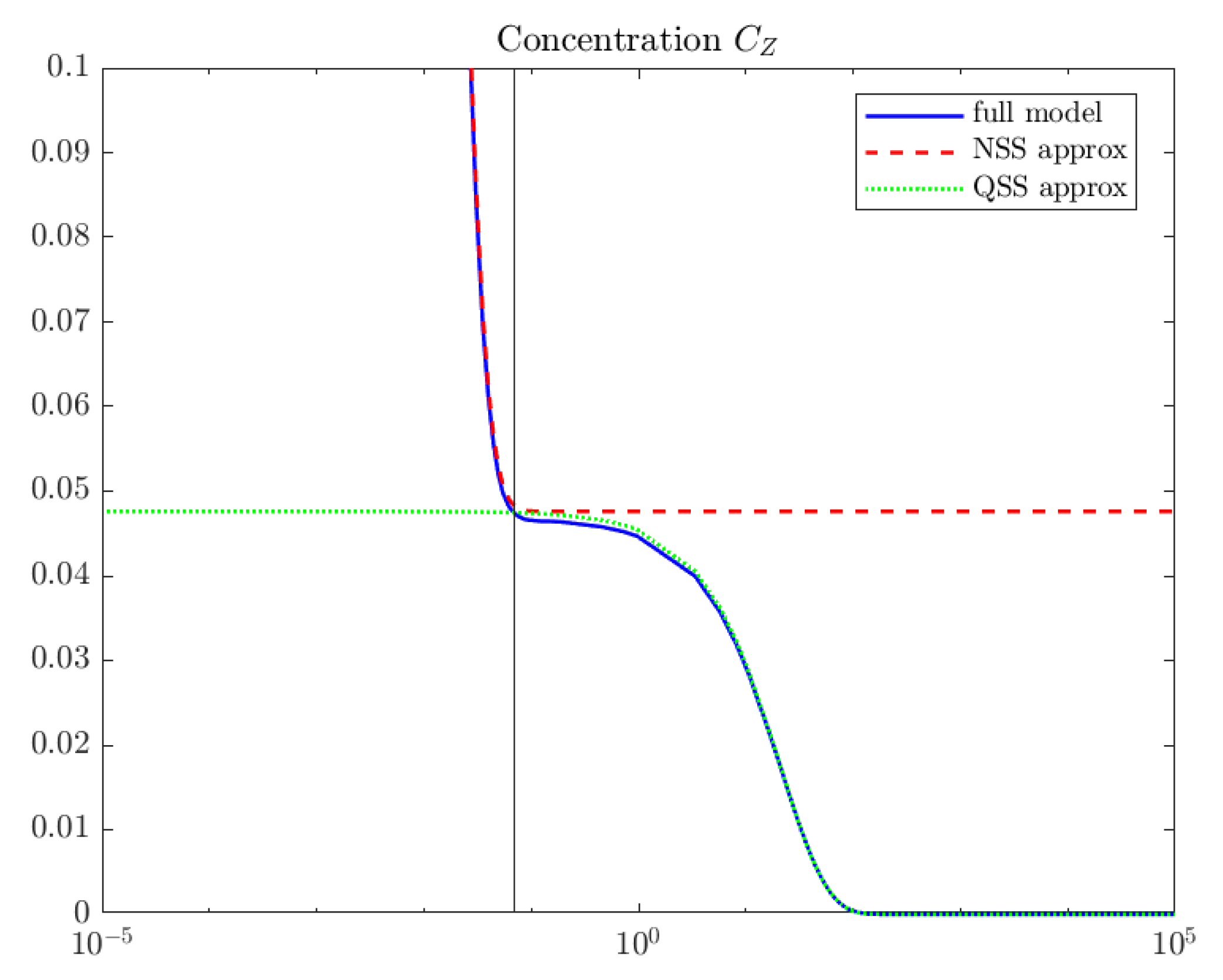
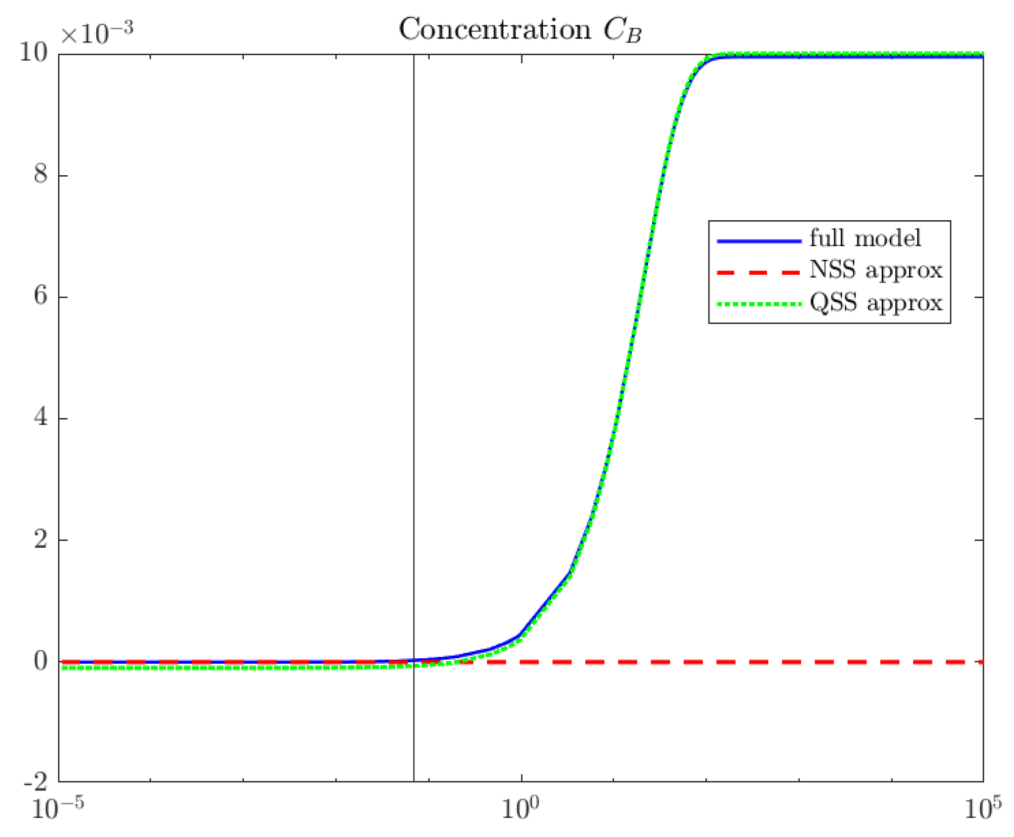
3.2. The Initial Non-Steady-State Domain; Gas Concentration Is Abundant, and Deactivation Is Negligible

Above we have introduced the full system of equations that will be studied further. We will first start with the implication of the two small parameters. If the small parameters are close to zero, i.e., ${\epsilon }_1,{\epsilon }_2\approx 0$ (or in the case of no deactivation ${\epsilon }_1\approx 0$ and ${\epsilon }_2=0$), then for small t we find that Equations (28) and (31) are approximately zero.

$$\begin{array}{cc}\hfill \frac{d{C}_{AZ}^{\prime }}{dt}=& k_1{N}_V{C}_A^{\prime }(N_S^{\prime }-C_{AZ}^{\prime })-k_2{C}_{AZ}^{\prime },\hfill \end{array}$$

(33)

$$\begin{array}{cc}\hfill \frac{d{N}_S^{\prime }}{dt}=& 0,\hfill \end{array}$$

(34)

$$\begin{array}{cc}\hfill C_Z^{\prime }=& N_S^{\prime }-C_{AZ}^{\prime },\hfill \\ \hfill \end{array}$$

(35)

$$\begin{array}{cc}\hfill \frac{d{C}_A^{\prime }}{dt}=& 0,\hfill \end{array}$$

(36)

$$\begin{array}{cc}\hfill C_B^{\prime }=& 1-C_A^{\prime }.\hfill \end{array}$$

(37)

If the change in active sites is approximately zero, this means there is almost no deactivation. On a certain domain where t is small we may claim there to be no deactivation. For the change in gas reactant A to be small, it has to be small compared to its absolute value. The change in A is insignificant because it is in abundance.

In this domain, for the full model, the changes in both substances (reactant A and active sites N) happen so slowly they cannot be observed, and thus are deemed insignificant. The fast behavior is dominating the slow one. Resulting in the following exact solution for the approximate model in the fast domain,

$$\begin{array}{cc}\hfill N_S^{\prime }\left(t\right)=& N_S^{\prime }\left(0\right)=1,\hfill \end{array}$$

(38)

$$\begin{array}{cc}\hfill C_A^{\prime }\left(t\right)=& C_A^{\prime }\left(0\right)=1,\hfill \end{array}$$

(39)

$$\begin{array}{cc}\hfill C_B^{\prime }\left(t\right)=& C_B^{\prime }\left(0\right)=0,\hfill \end{array}$$

(40)

$$\begin{array}{cc}\hfill C_{AZ}^{\prime }\left(t\right)=& \frac{k_1{N}_V}{k_1{N}_V+k_2}(1-exp\left(-(k_1{N}_V+k_2)t\right),\hfill \end{array}$$

(41)

$$\begin{array}{cc}\hfill C_Z^{\prime }\left(t\right)=& \frac{k_2}{k_1{N}_V+k_2}+\frac{k_1{N}_V}{k_1{N}_V+k_2}exp\left(-(k_1{N}_V+k_2)t\right).\hfill \end{array}$$

(42)

$$\frac{C_{AZ}^{\prime }}{C_Z^{\prime }}=\frac{k_1{N}_V-k_1{N}_{V}exp\left(-(k_1{N}_V+k_2)t\right)}{k_2+k_1{N}_{V}exp\left(-(k_1{N}_V+k_2)t\right)}$$

(43)

The fast domain, also referred to as the non-steady-state (NSS) domain, is the time frame in which the above solutions are good estimates for the exact solutions. It is governed by the main catalytic cycle with “no” deactivation and under the assumption that the gas concentration is abundant.

3.3. The Quasi-Steady-State Domain; Deactivation Is Absent

When we go outside the fast or non-steady-state (NSS) domain, the same assumptions don’t hold as in the previous section. Here we need to differentiate whether deactivation is truly absent or not. We first look at the case where deactivation is absent, i.e., ${\epsilon }_2=0$.

In this slow domain, we introduce the new time $\tau ={\epsilon }_{1}t$. The main result of introducing the time $\tau$ with small parameter ${\epsilon }_1$ is the following equations for the catalytic intermediates,

$$\begin{array}{cc}\hfill {\epsilon }_1\frac{d{C}_{AZ}^{\prime }}{d\tau }=& k_1{N}_V\left(C_A^{\prime }(N_S^{\prime }-C_{AZ}^{\prime })-\frac{k_2}{k_1{N}_V}{C}_{AZ}^{\prime }\right),\hfill \end{array}$$

(44)

$$\begin{array}{cc}\hfill C_Z^{\prime }=& N_S^{\prime }-C_{AZ}^{\prime }.\hfill \end{array}$$

(45)

Since ${\epsilon }_1\approx 0$, we can replace Equation (44) with the algebraic equation,

$$k_1{N}_V\left(C_A^{\prime }(N_S^{\prime }-C_{AZ}^{\prime })-\frac{k_2}{k_1{N}_V}{C}_{AZ}^{\prime }\right)=0.$$

(46)

This is our quasi-steady-state (QSS) assumption, and we identify this domain as the QSS domain. The QSS intermediate concentrations are calculated as,

$$\begin{array}{cc}\hfill C_{AZ}^{\prime }=& \frac{k_1{N}_V{C}_A^{\prime }}{k_1{N}_V{C}_A^{\prime }+k_2}{N}_S^{\prime },\hfill \end{array}$$

(47)

$$\begin{array}{cc}\hfill C_Z^{\prime }=& \frac{k_2}{k_1{N}_V{C}_A^{\prime }+k_2}{N}_S^{\prime }.\hfill \end{array}$$

(48)

If we substitute the values of $C_A^{\prime }$ and $N_S^{\prime }$ with their respective ‘fresh’ values $C_{A,fresh}^{\prime }=C_A^{\prime }\left(0\right)$ and $N_{S,fresh}^{\prime }=N_S^{\prime }\left(0\right)$ these solutions are equivalent to the steady-state (SS) values of Equation (41) and Equation (42) respectively.

At the beginning of the QSS domain, the concentration $C_A$ is changing insignificantly and the relative ratio composition of the active catalyst sites,

$$\frac{C_{AZ}^{\prime }}{C_Z^{\prime }}=\frac{k_1{N}_V{C}_A^{\prime }}{k_2},$$

(49)

appears constant. However, as time increases the change in $C_A$ will increase, and thus the ratio will not remain constant. As we will see in later sections this is not the case when deactivation is present.

3.3.1. Introduction to the Lambert W function

To recap, in the absence of deactivation, we have the following set of equations for the dimensionless concentrations,

$$\begin{array}{cc}\hfill {\epsilon }_1\frac{d{C}_{AZ}^{\prime }}{d\tau }=& k_1{N}_V{C}_A^{\prime }(N_S^{\prime }-C_{AZ}^{\prime })-k_2{C}_{AZ}^{\prime },\hfill \end{array}$$

(50)

$$\begin{array}{cc}\hfill C_Z^{\prime }=& N_S^{\prime }-C_{AZ}^{\prime },\hfill \\ \hfill \end{array}$$

(51)

$$\begin{array}{cc}\hfill \frac{d{C}_A^{\prime }}{d\tau }=& -k_1{N}_V{C}_A^{\prime }(N_S^{\prime }-C_{AZ}^{\prime }),\hfill \end{array}$$

(52)

$$\begin{array}{cc}\hfill C_B^{\prime }=& 1-C_A^{\prime }-{\epsilon }_1{C}_{AZ}^{\prime }.\hfill \end{array}$$

(53)

There are two nonlinear differential equations, (50) and (52), and two linear algebraic equations, (51) and (53). Making use of the small parameter and the quasi-steady-state (QSS) assumption, see Equations (46)–(48), this set of equations reduce to one nonlinear differential equation, (56), and three algebraic equations, (54), (55) and (57).

$$\begin{array}{cc}\hfill C_{AZ}^{\prime }=& \frac{k_1{N}_V{C}_A^{\prime }}{k_1{N}_V{C}_A^{\prime }+k_2}{N}_S^{\prime },\hfill \end{array}$$

(54)

$$\begin{array}{cc}\hfill C_Z^{\prime }=& \frac{k_2}{k_1{N}_V{C}_A^{\prime }+k_2}{N}_S^{\prime },\hfill \end{array}$$

(55)

$$\begin{array}{cc}\hfill \frac{d{C}_A^{\prime }}{d\tau }=& -\frac{k_1{k}_2{N}_V{C}_A^{\prime }}{k_1{N}_V{C}_A^{\prime }+k_2}{N}_S^{\prime },\hfill \end{array}$$

(56)

$$\begin{array}{cc}\hfill C_B^{\prime }=& 1-C_A^{\prime }-{\epsilon }_1\frac{k_1{N}_V{C}_A^{\prime }}{k_1{N}_V{C}_A^{\prime }+k_2}{N}_S^{\prime }.\hfill \end{array}$$

(57)

This specific set of equations is well-known in the literature. However, to our knowledge, an exact analytical expression for the concentration of A has yet to be presented.

To this end, we would like to introduce the Lambert W function [40], which calculates the converse (inverse) relation of the function

$$f\left(w\right)=w{e}^w,$$

with $w\in \mathbb{C}$.

We now have a way to express the solution of ordinary differential Equation (56),

$$\begin{array}{cc}\hfill C_A^{\prime }\left(\tau \right)=& exp\left(-\mathrm{LambertW}\left(\frac{1}{\eta }exp\left(-\frac{1}{\eta }(k_2{N}_S^{\prime }t-1)\right)\right)-\frac{1}{\eta }(k_2{N}_S^{\prime }t-1)\right),\hfill \end{array}$$

(58)

$$\begin{array}{cc}\hfill \eta =& \frac{k_2}{k_1{N}_V}.\hfill \end{array}$$

(59)

Remember because there is no deactivation $N_S$ will be constant and $N_S^{\prime }=1$ for all time. By extension of the above equation we now also have analytical expressions for the remaining concentrations,

$$\begin{array}{cc}\hfill C_{AZ}^{\prime }\left(\tau \right)=& \frac{k_1{N}_V{C}_A^{\prime }\left(\tau \right)}{k_1{N}_V{C}_A^{\prime }\left(\tau \right)+k_2}\hfill \end{array}$$

(60)

$$\begin{array}{cc}\hfill C_Z^{\prime }\left(\tau \right)=& \frac{k_2}{k_1{N}_V{C}_A^{\prime }\left(\tau \right)+k_2}\hfill \end{array}$$

(61)

$$\begin{array}{cc}\hfill C_B^{\prime }\left(\tau \right)=& 1-C_A\left(\tau \right)\left(1-{\epsilon }_1\frac{k_1{N}_V}{k_1{N}_V{C}_A^{\prime }\left(\tau \right)+k_2}\right)\hfill \end{array}$$

(62)

$$R\left(\tau \right)=k_2{C}_{AZ}=k_2{C}_{AZ}^{\prime }{N}_S=N_S\frac{k_1{k}_2{N}_V{C}_A^{\prime }\left(\tau \right)}{k_1{N}_V{C}_A^{\prime }\left(\tau \right)+k_2}$$

(63)

Using Equation (58), one can obtain the expression for half decay time, ${\tau }_{1/2}$, which is traditional in chemical kinetics. It is the time during which half of the reactant is transformed into the product.

As known, for the first order reaction $\mathrm{A}\stackrel{\mathrm{k}}{\to }\mathrm{B}$,

$${\tau }_{1/2}=\frac{ln\left(2\right)}{k}$$

where k is the kinetic rate coefficient of the reaction. For our two-step mechanism (Temkin–Boudart mechanism), based on Equation (58),

$${\tau }_{1/2}=\frac{ln\left(2\right)}{k_1{N}_V}+\frac{1}{2k_2}$$

(64)

Clearly, the half decay time is decreased with the rise of both kinetic coefficients $k_1{N}_V$ and $k2$. If $k_2$ is much bigger then $k_1{N}_V$,

$${\tau }_{1/2}=\frac{ln\left(2\right)}{k_1{N}_V},$$

(65)

it is identical to the expression for the first-order reaction. In contrast, if $k_1{N}_V$ is much bigger than $k_2$ then,

$${\tau }_{1/2}=\frac{1}{2k_2}.$$

(66)

If $k_1{N}_V=k_2=k$,

$${\tau }_{1/2}=\frac{1/2+ln\left(2\right)}{k}\approx \frac{1.19}{k}.$$

(67)

This expression can be used as a rough estimate of the parameter.

Based on Equation (64) it is possible to recognize the deviation of the Temkin–Boudart non-steady-state kinetic dependence from the first-order (linear) one.

3.4. The Quasi-Steady-State Domain of the Cyclic Reaction Accompanied by Deactivation

In this domain, applying the quasi-steady-state assumption, the kinetic model is given by:

$$\begin{array}{cc}\hfill C_{AZ}^{\prime }=& \frac{k_1{N}_V{C}_A^{\prime }}{k_1{N}_V{C}_A^{\prime }+k_2}{N}_S^{\prime },\hfill \end{array}$$

(68)

$$\begin{array}{cc}\hfill C_Z^{\prime }=& \frac{k_2}{k_1{N}_V{C}_A^{\prime }+k_2}{N}_S^{\prime },\hfill \end{array}$$

(69)

$$\begin{array}{cc}\hfill \frac{d{N}_S^{\prime }}{d\tau }=& -\frac{{\epsilon }_2}{{\epsilon }_1}\frac{k_1{k}_2{N}_V}{k_1{N}_V{C}_A^{\prime }+k_2}{N}_S^{\prime },\hfill \end{array}$$

(70)

$$\begin{array}{cc}\hfill \frac{d{C}_A^{\prime }}{d\tau }=& -\frac{k_1{k}_2{N}_V{C}_A^{\prime }}{k_1{N}_V{C}_A^{\prime }+k_2}{N}_S^{\prime },\hfill \end{array}$$

(71)

$$\begin{array}{cc}\hfill C_B^{\prime }=& 1-C_A^{\prime }-{\epsilon }_1\frac{k_1{N}_V{C}_A^{\prime }}{k_1{N}_V{C}_A^{\prime }+k_2}{N}_S^{\prime }.\hfill \end{array}$$

(72)

This system of equations consists out of two nonlinear differential equations, (70) and (71), and three algebraic equations, (68), (69) and (72).

We can rewrite the two differential equations above into one nonlinear differential equation,

$$\frac{d{N}_S^{\prime }}{d{C}_A^{\prime }}=\frac{{\epsilon }_2}{{\epsilon }_1{C}_A^{\prime }}.$$

(73)

The analytical solution to Equation (73) is found to be

$$N_S^{\prime }\left(C_A^{\prime }\right)=\frac{{\epsilon }_2}{{\epsilon }_1}ln\left(C_A^{\prime }\right).$$

(74)

This equation, while correct, does not give much information about the progression of the dimensionless concentration of active sites $N_S^{\prime }$. The three-factor kinetic equation, (11) as it is presented in [11], can be adapted for models without reversible deactivation by setting ${\phi }_{r,d}=1$ and $K_d=1$ (Appendix A describes the conditions under which we may use the three-factor rate equation). This results in the following rate equation for this domain,

$$\begin{array}{cc}\hfill R\left(\tau \right)=& k_2{C}_{AZ}=k_2{C}_{AZ}^{\prime }{N}_S^0,\hfill \\ \hfill \approx & N_S^0{R}_{\mathrm{fresh}}{\phi }_{i,d},\hfill \\ \hfill =& \frac{k_1{k}_2{N}_V{C}_{A,fresh}^{\prime }}{k_1{N}_V{C}_{A,fresh}^{\prime }+k_2}{N}_S^{0}exp\left(-\frac{{\epsilon }_2}{{\epsilon }_1}\frac{k_1{k}_2{N}_V}{k_1{N}_V{C}_{A,fresh}^{\prime }+k_2}\tau \right).\hfill \end{array}$$

(75)

First, we simplify the terms inside the exponential as follows,

$$\begin{array}{cc}\hfill C_{Z,\mathrm{fresh}}^{\prime }=& \frac{k_2}{k_1{N}_V{C}_{A,fresh}+k_2},\hfill \end{array}$$

(76)

$$\begin{array}{cc}\hfill {\epsilon }_2=& \frac{k_d}{k_1{N}_V},\hfill \end{array}$$

(77)

$$\begin{array}{cc}\hfill R\left(\tau \right)=& \frac{k_1{k}_2{N}_V{C}_{A,fresh}^{\prime }}{k_1{N}_V{C}_{A,fresh}^{\prime }+k_2}{N}_S^{0}exp\left(-\frac{k_d}{{\epsilon }_1}{C}_{Z,\mathrm{fresh}}^{\prime }\tau \right).\hfill \end{array}$$

(78)

Now we shift our time out of the “slow” time $\tau$ domain to the “fast” time t one, which results in the final expression for the rate equation,

$$\begin{array}{cc}\hfill \tau =& {\epsilon }_{1}t,\hfill \end{array}$$

(79)

$$\begin{array}{cc}\hfill R\left(t\right)=& \frac{k_1{k}_2{N}_V{C}_{A,fresh}^{\prime }}{k_1{N}_V{C}_{A,fresh}^{\prime }+k_2}{N}_S^{0}exp\left(-k_d{C}_{Z,\mathrm{fresh}}^{\prime }t\right).\hfill \end{array}$$

(80)

Obviously, $k_d{C}_{Z,\mathrm{fresh}}^{\prime }$ is the rate of deactivation for the fresh catalyst. Therefore, the phenomenological equation can be written as,

$$R\left(t\right)=R_{\mathrm{fresh}}{e}^{-R_{d}t},$$

(81)

where $R_d=k_d{C}_{Z,\mathrm{fresh}}^{\prime }$ is the rate of deactivation of the fresh catalyst.

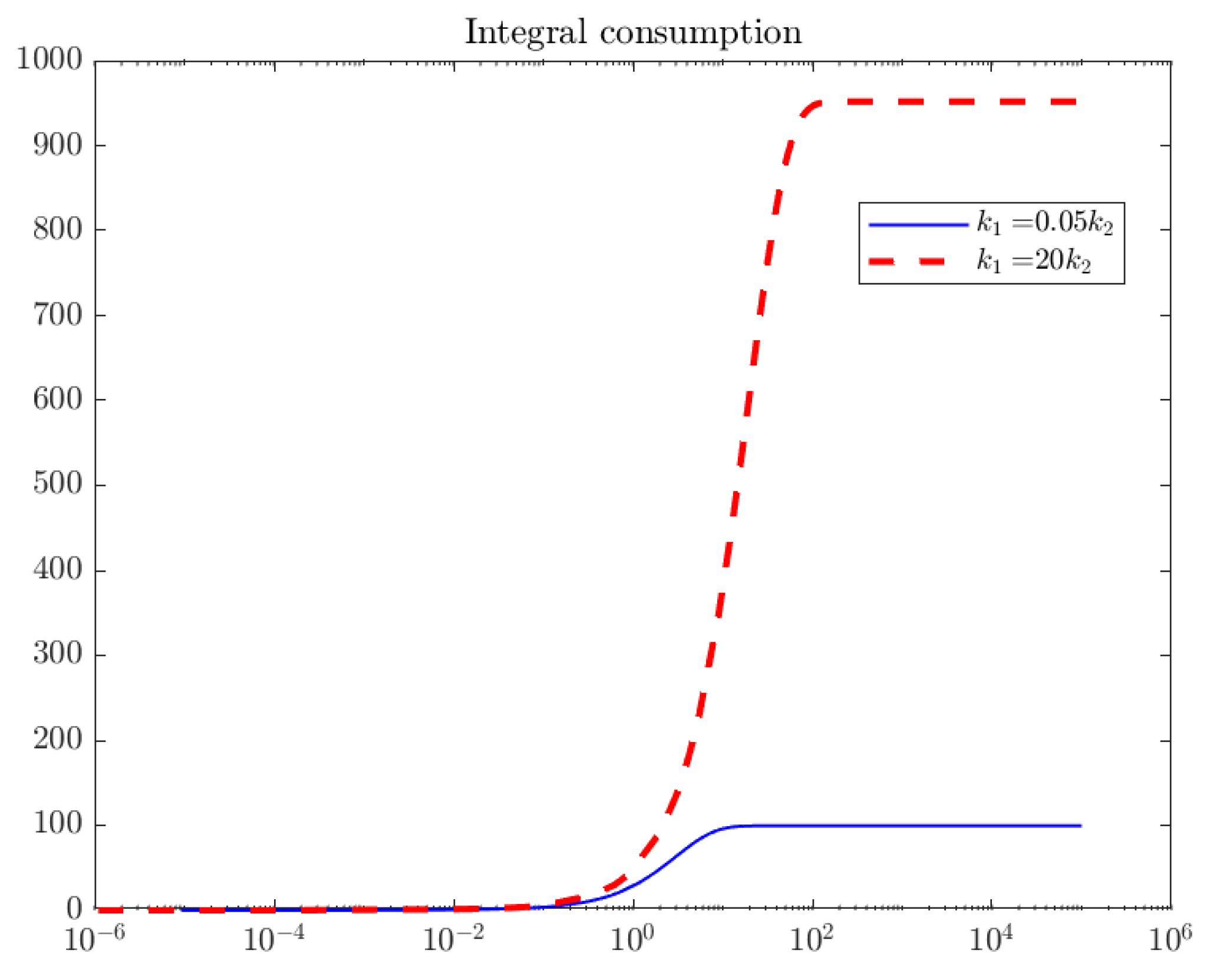
3.5. Integral Consumption

The integral consumption of the reactant which we are going to obtain and analyze is expressed as,

$$\begin{array}{cc}\hfill A\left(t\right)=& {\int }_0^{t}R\left(x\right)dx,\hfill \\ \hfill A\left(t\right)=& N_S^0\frac{k_1{N}_V{C}_A^{\prime }\left(t\right)}{k_d}\left(1-exp\left(-k_d{C}_{Z,\mathrm{fresh}}^{\prime }t\right)\right).\hfill \end{array}$$

(82)

Experimentally, in the quasi-steady-state domain the dependence of $A\left(t\right)$ can be measured by the change of concentrations in time of reactant A ($\Delta C_A$) or product B ($\Delta C_B$) multiplied by the factor ($\frac{V_{\mathrm{gas}}}{S_{\mathrm{cat}}}$). In our case, where the change in the reactant concentration is insignificant, the product concentrations are more convenient for calculating the values of $A\left(t\right)$.

There are two extreme cases for the integral consumption equation:

• The limit of the integral consumption as time goes to infinity, $t\to \infty$,

  $$A_{\lim }=N_S^0\frac{k_1{N}_V{C}_A^{\prime }}{k_d}.$$

  (83)
  We find the limit of integral consumption is equal to the product of the number of active sites for the fresh catalyst multiplied by the ratio of the kinetic coefficients of the two reactions competing for the free active site Z. One reaction belongs to the catalytic cycle,
  $$\mathrm{A}+\mathrm{Z}\stackrel{k1}{\to }\mathrm{AZ}.$$

  The other reaction belongs to the irreversible deactivation step,
  $$\mathrm{Z}\stackrel{kd}{\to }\mathrm{X}.$$
• The Taylor approximation for $A\left(t\right)$ at small values of $k_{d}t$. If the term $k_{d}t$ is very small, i.e., $k_{d}t\ll 1$, the Taylor approximation of $A\left(t\right)$ will be

  $$\begin{array}{cc}\hfill A\left(t\right)=& N_S^0\frac{k_1{N}_V{C}_A^{\prime }}{k_d}(1-(1-k_d{C}_{Z,\mathrm{fresh}}^{\prime }t))+\mathcal{O}\left(k_{d}t\right),\hfill \\ \hfill \approx & R_{\mathrm{fresh}}t.\hfill \end{array}$$

  (84)

3.6. Combining the Integral Consumption and the Quasi-Steady-State Equation Rate

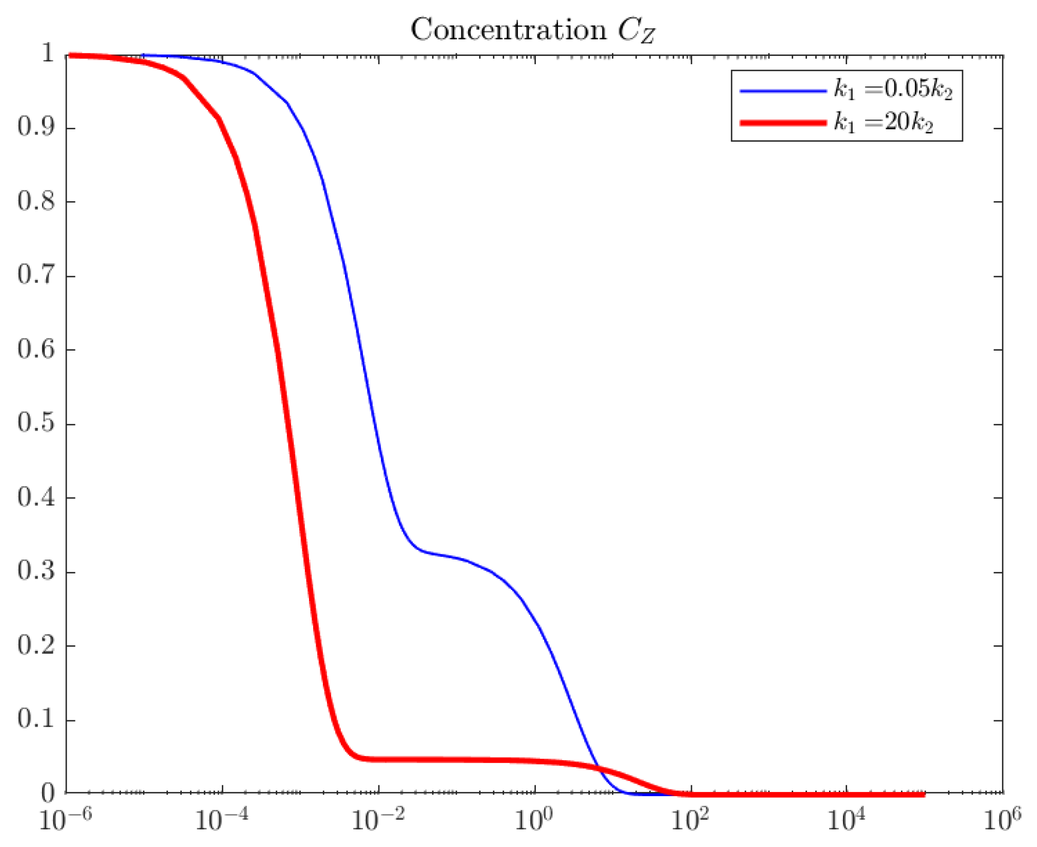
Comparing the equations for the limit of the integral consumption (83) and the equation for the quasi-steady-state rate, we obtain

$$\frac{A_{\lim }}{R_{\mathrm{fresh}}}=\frac{1}{C_{Z,\mathrm{fresh}}^{\prime }}\frac{1}{k_d}.$$

(85)

This ratio $\frac{A_{\lim }}{R_{\mathrm{fresh}}}$ can be interpreted as the catalyst lifetime for the catalytic reaction with deactivation,

$${\tau }_{\mathrm{cat}}=\frac{A_{\lim }}{R_{\mathrm{fresh}}}.$$

(86)

If $k_1{N}_V{C}_A^{\prime }\gg k_2$ then

$${\tau }_{\mathrm{cat}}\approx \frac{k_1{N}_V{C}_A^{\prime }}{k_2}\frac{1}{k_d}.$$

If $k_1{N}_V{C}_A^{\prime }\ll k_2$ then

$${\tau }_{\mathrm{cat}}\approx \frac{1}{k_d}.$$

4. Computations

Figure 2 shows the evolution of the concentration of free active sites which first dramatically decreases, then exhibits a plateau, and finally decreases gradually to zero.

Interestingly, this whole model is characterized by a temporal turning point. Left of this turning point, the whole model can easily be approximated by the NSS no-deactivation model. Regarding this point, the QSS model with deactivation (not without) is an excellent approximation of the whole model.

This turning point corresponds to the ‘fresh’ catalyst, which is characterized by the QSS surface composition.

Under the values of our parameters, the concentration of reactants changes insignificantly in all temporal intervals (the case of small conversion). The concentration of product B is presented in Figure 3.

In our case, the non-steady-state (NSS) domain with deactivation is characterized by the insignificant contribution of reactant A. Furthermore, the effect of deactivation on the concentration of the intermediate is insignificant as well in this domain. The NSS with the no-deactivation domain is indistinguishable from the domain with deactivation.

As for the QSS domain, the main catalytic cycle is accompanied by deactivation from the very beginning of this domain.

Figure 4 and Figure 5 illustrate the main theoretical result of our paper: that if we increase the rate coefficient $k_1$, this will result in a decrease of the QSS concentration of free active sites $C_Z$. Consequently, the integral consumption of reactant A and its limit $A_{\lim }$ will increase, where $A_{\lim }$’s increase will be proportional to the increase in the rate coefficient $k_1$. Hence, the lifetime of the catalyst ${\tau }_{\mathrm{cat}}$ will increase as well.

5. Interpretation and Discussion

The concept of the integral reactant consumption for the catalytic cyclic reaction accompanied by deactivation became the basis for deriving the corresponding analytical expressions.

These expressions, i.e., the integral reactant assumption and catalyst lifetime as a function of reaction parameters, are important for formulating a new general strategy in the optimization of these reactions or processes.

Equations (83) and (86) propose the following recipe for intensifying the catalytic process and extending the catalyst life. The concentration of free active sites (so to say, the deactivated catalytic intermediate) must be kept as low as possible.

It can be achieved by increasing the reactant concentration $C_A$ which reacts with the intermediate Z (free active site). In our case, this is reactant A.

It has arisen a reasonable question: “What about the justification of this recommendation?”

In the monograph “Homogeneous Catalysis with Metal Complexes: Kinetic Aspects and Mechanisms” by O.N. Temkin and P.P. Pozdeev [41], there is a special section devoted to this problem “5.3.5. Protecting active centers by catalytic process from destruction” pp. 492–493. The pioneering paper by Kagan et al. [42] was referred. The observed phenomenon is described as follows: in the reaction of hydroformylation of olefines catalyzed by Rh complexes, the high rate of transformation of the active complex, [HRh($\mathrm{C}{\mathrm{O}}_3$)], leads to the decrease in the steady-state concentration of this complex. As result, the deactivation of this complex by the cluster generation is hindered. So, we can consider this publication as an experimental justification of the phenomenon, i.e., an enhancement of the catalyst lifetime by the decrease of the steady-state concentration of the free active sites. However, the theoretical analysis related to this phenomenon was still not done, and its corresponding relationships are absent.

6. Conclusions and Perspectives

In this paper, for the basic catalytic two-step mechanism (Temkin–Boudart mechanism) with irreversible reactions and irreversible deactivation, two analytical results have been obtained, i.e., the expression for the integral consumption of the gas substance and the expression for the catalyst lifetime. These results became a basis for distinguishing the new phenomenon, the enhancement of the catalytic reaction with deactivation via the regime with the small steady-state concentration of free active sites. In some domain of parameters, it can be achieved by increasing the steady-state (quasi-steady-state) reaction rate of the fresh catalyst. We can express this conclusion as follows: under some conditions, the elevated fresh catalyst activity protects the catalyst from deactivation. These analytical results are illustrated by computer calculations.

We consider these results as prototypes of analogous results for similar models mentioned in the introduction of this paper, i.e., two-step mechanism and n-step single route linear mechanism with reversible steps, models with reversible deactivation, and models of reactions in the CSTR. For some of these models, we already have preliminary results and are going to develop them more applying this approach to the description of the experimental kinetic data with catalyst deactivation.

On the other side, the idea of “protecting active centers from deactivation by catalytic process” can be used heuristically for the intensification of the catalytic process.

References

1. Szépe, S.; Levenspiel, O. Optimal temperature policies for reactors subject to catalyst deactivation—I Batch reactor. Chem. Eng. Sci. 1968, 23, 881–894. [Google Scholar] [CrossRef]
2. Corella, J.; Asua, J. Kinetic equations of mechanistic type with nonseparable variables for catalyst deactivation by coke. Models and data analysis methods. Ind. Eng. Chem. Process Des. Dev. 1982, 21, 55–61. [Google Scholar] [CrossRef]
3. Corella, J.; Adanez, J.; Monzon, A. Some intrinsic kinetic equations and deactivation mechanisms leading to deactivation curves with a residual activity. Ind. Eng. Chem. Res. 1988, 27, 375–381. [Google Scholar] [CrossRef]
4. Froment, G.; Bischoff, K. Non-steady state behaviour of fixed bed catalytic reactors due to catalyst fouling. Chem. Eng. Sci. 1961, 16, 189–201. [Google Scholar] [CrossRef]
5. Froment, G.; Bischoff, K. Kinetic data and product distributions from fixed bed catalytic reactors subject to catalyst fouling. Chem. Eng. Sci. 1962, 17, 105–114. [Google Scholar] [CrossRef]
6. Beeckman, J.; Froment, G. Catalyst deactivation by site coverage and pore blockage: Finite rate of growth of the carbonaceous deposit. Chem. Eng. Sci. 1980, 35, 805–815. [Google Scholar] [CrossRef]
7. Marin, G.; Beeckman, J.; Froment, G. Rigorous kinetic models for catalyst deactivation by coke deposition: Application to butene dehydrogenation. J. Catal. 1986, 97, 416–426. [Google Scholar] [CrossRef]
8. Tsheglove, G.; Gel’bshtein, A.; Yablonskii, G.; Kamenko, B. Dynamic kinetic model of vinyl chlorice synthesis. Ind. Eng. Chem. Res. 1972, 27, 709–718. [Google Scholar]
9. Butt, J.; Petersen, E. Activation, Deactivation and Poisoning of Catalysts; Academic Press: San Diego, CA, USA, 1988; 495p. [Google Scholar]
10. Bartholomew, C. Mechanisms of catalyst deactivation. Appl. Catal. Gen. 2001, 212, 17–60. [Google Scholar] [CrossRef]
11. Gromotka, Z.; Yablonsky, G.; Ostrovskii, N.; Constales, D. Three-Factor Kinetic Equation of Catalyst Deactivation. Entropy 2021, 23, 818. [Google Scholar] [CrossRef]
12. Ostrovskii, N.; Yablonskii, G. Kinetic equation for catalyst deactivation. React. Kinet. Catal. Lett. 1989, 39, 287–292. [Google Scholar] [CrossRef]
13. Ostrovskii, N. Catalyst Deactivation Kinetics: Mathematical Models and Their Applications; NAUKA: Moscow, Russia, 2001; 334p. (In Russian) [Google Scholar]
14. Ostrovskii, N. General equation for linear mechanisms of catalyst deactivation. Chem. Eng. J. 2006, 120, 73–82. [Google Scholar] [CrossRef]
15. Yablonsky, G.; Constales, D.; Marin, G. Single-Route Linear Catalytic Mechanism: A New, Kinetico-Thermodynamic Form of the Complex Reaction Rate. Symmetry 2020, 12, 1748. [Google Scholar] [CrossRef]
16. Cordero-Lanzac, T.; Aguayo, A.; Gayubo, A.; Castaño, P.; Bilbao, J. Simultaneous modeling of the kinetics for n-pentane cracking and the deactivation of a HZSM-5 based catalyst. Chem. Eng. J. 2018, 331, 818–830. [Google Scholar] [CrossRef]
17. Cordero-Lanzac, T.; Hita, I.; Garcia-Mateos, F.; Castaño, P.; Rodriguez-Mirasol, J.; Cordero, T.; Bilbao, J. Adaptable kinetic model for the transient and pseudo-steady states in the hydrodeoxygenation of raw bio-oil. Chem. Eng. J. 2020, 400, 124679. [Google Scholar] [CrossRef]
18. Cordero-Lanzac, T.; Aguayo, A.; Gayubo, A.; Castaño, P.; Bilbao, J. A comprehensive approach for designing different configurations of isothermal reactors with fast catalyst deactivation. Chem. Eng. J. 2020, 379, 122260. [Google Scholar] [CrossRef]
19. Bodenstein, M. Eine theorie der photochemischen reaktionsgeschwindigkeiten. Zeitschrift für Physikalische Chemie 1913, 85, 329–397. [Google Scholar] [CrossRef] [Green Version]
20. Chapman, D.; Underhill, L. The interaction of chlorine and hydrogen. The influence of mass. J. Chem. Soc. Trans. 1913, 103, 496–508. [Google Scholar] [CrossRef] [Green Version]
21. Christiansen, J. The elucidation of reaction mechanisms by the method of intermediates in quasi-stationary concentrations. Adv. Catal. 1953, 5, 311–353. [Google Scholar]
22. Yablonskii, G.; Bykov, V.; Elokhin, V.; Gorban, A. Kinetic Models of Catalytic Reactions; Elsevier: Amsterdam, The Netherlands, 1991; Volume 32, 396p. [Google Scholar]
23. Marin, G.; Yablonsky, G.; Constales, D. Kinetics of Chemical Reactions: Decoding Complexity; Wiley-VCH: Weinheim, Germany, 2019; 442p. [Google Scholar]
24. Michaelis, L.; Menten, M. Die kinetik der Invertinwirkung. Biochem. Z 1913, 49, 352. [Google Scholar]
25. Gorban, A.; Shahzad, M. The Michaelis–Menten–Stueckelberg theorem. Entropy 2011, 13, 966–1019. [Google Scholar] [CrossRef] [Green Version]
26. Briggs, G.; Haldane, J. A note on the kinetics of enzyme action. Biochem. J. 1925, 19, 338. [Google Scholar] [CrossRef] [PubMed] [Green Version]
27. Tikhonov, A. Systems of differential equations containing small parameters in the derivatives. Matematicheskii Sbornik 1952, 73, 575–586. [Google Scholar]
28. Sayasov, Y.; Vasil’eva, A. Semenov-Bodenstein’s method of quasi-steady-state concentrations: Justification and applicability to the gas chain reaction. Zh. Fiz. Khim. 1955, 29, 802–810. [Google Scholar]
29. Butuzov, V.; Vasil’eva, A. Asymptotic Expansions for Singularly Perturbed Equations; NAUKA: Moscow, Russia, 1973. [Google Scholar]
30. Tikhonov, N.; Vasil’eva, A.; Sveshnikov, A. Differential Equations; Springer: New York, NY, USA, 1985. [Google Scholar]
31. Bowen, J.; Acrivos, A.; Oppenheim, A. Singular perturbation refinement to quasi-steady state approximation in chemical kinetics. Chem. Eng. Sci. 1963, 18, 177–188. [Google Scholar] [CrossRef]
32. Heineken, F.; Tsuchiya, H.; Aris, R. On the mathematical status of the pseudo-steady state hypothesis of biochemical kinetics. Math. Biosci. 1967, 1, 95–113. [Google Scholar] [CrossRef]
33. Yablonskii, G.; Bykov, V.; Gorban, A. Mathematical Models of Catalytic Reactions; Nauka: Novsibirsk, Russia, 1983. [Google Scholar]
34. Gorban, A.; Karlin, I. Method of invariant manifold for chemical kinetics. Chem. Eng. Sci. 2003, 58, 4751–4768. [Google Scholar] [CrossRef] [Green Version]
35. Gorban, A.; Radulescu, O.; Zinovyev, A. Asymptotology of chemical reaction networks. Chem. Eng. Sci. 2010, 65, 2310–2324. [Google Scholar] [CrossRef] [Green Version]
36. Gorban, A. Model reduction in chemical dynamics: Slow invariant manifolds, singular perturbations, thermodynamic estimates, and analysis of reaction graph. Curr. Opin. Chem. Eng. 2018, 21, 48–59. [Google Scholar] [CrossRef] [Green Version]
37. Temkin, M. Relaxation rate of two-stage catalytic reaction. Kinetica Catal. 1976, 17, 945–949. [Google Scholar]
38. Boudart, M. Two-step catalytic reactions. AIChE J. 1972, 18, 465–478. [Google Scholar] [CrossRef]
39. Marin, G.; Galvita, V.; Yablonsky, G. Kinetics of chemical processes: From molecular to industrial scale. J. Catal. 2021, 404, 745–759. [Google Scholar] [CrossRef]
40. Mezo, I. The Lambert W Function: Its Generalizations and Applications; Chapman and Hall/CRC: New York, NY, USA, 2022. [Google Scholar] [CrossRef]
41. Temkin, O.; Pozdeev, P. Homogeneous Catalysis with Metal Complexes: Kinetic Aspects and Mechanisms; John Wiley & Sons: Hoboken, NJ, USA, 2012; 860p. [Google Scholar]
42. Kagan, Y.; Rozovskij, A.; Slivinskij, E.; Korneeva, G. Autoregulatory effect in the hydroformylation reaction of olefins. Kinetika I Kataliz 1987, 28, 1508–1511. [Google Scholar]
Figure 1. The three-building-block scheme approach to phenomenological modeling for a linear catalytic reaction accompanied by linear catalyst deactivation. Block one is a n-step linear catalytic reaction. Block two is a linear reversible catalyst deactivation. Block three is aging, i.e., linear irreversible catalyst deactivation.
Catalysts 12 01283 g001
Figure 2. Concentration of Z.
Catalysts 12 01283 g002
Figure 3. Concentration of B.
Catalysts 12 01283 g003
Figure 4. Concentration C Z for different k 1 .
Catalysts 12 01283 g004
Figure 5. Integral consumption for different k 1 .
Catalysts 12 01283 g005
Publisher’s Note: MDPI stays neutral with regard to jurisdictional claims in published maps and institutional affiliations.