A Machine Learning Approach for Efficient Selection of Enzyme Concentrations and Its Application for Flux Optimization

 , , ,
, , ,
Abstract
:
1. Introduction
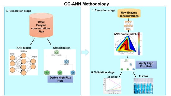
2. Methodology
2.1. Data for New Methodology
2.2. ANN-Based Flux Prediction Workflow
2.2.1. Preparation stage
Reduction of Data Dimensionality
Visualization of Data
Classification of Data for Higher Flux (> 12 µM/s)
Neural Network Model
2.2.2. Execution Stage
Generation of New Enzyme Concentration
Flux Prediction Using ANN
2.2.3. Validation of Methodology
Simulation of Upper Part of Glycolysis
Experimental Validation
2.2.4. The Workflow of the Proposed Methodology
3. Application and Results
3.1. Preparation
3.1.1. Data Dimension Reduction
3.1.2. Visualization of Data
3.1.3. Enzyme Concentration Rule
3.1.4. Neural Network Model
3.2. Execution
3.2.1. Generation of New Enzyme Concentrations
3.2.2. Flux Prediction Using ANN
3.3. Validation
3.3.1. Simulation of Upper Part of Glycolysis
3.3.2. Experimental Validation of the Methodology
Enzyme Assays for Measurement of Kinetic Parameters
Flux Determinations
3.4. Application: Selection of Cost-Efficient Enzyme Balances
4. Discussion
4.1. GC-ANN Approach Could be Used to Predict “Out-of-the-Box” Values
4.1.1. In-Silico Validation
4.1.2. In Vitro Validation
4.2. The Proposed Methodology Is Cost-Efficient
5. Materials and Methods
5.1. Determination of Protein Concentration
5.2. Enzyme Assays for the Determination of Kinetic Parameters
5.3. Flux Measurements
6. Conclusions
Supplementary Materials
Author Contributions
Funding
Conflicts of Interest
Availability of Data and Materials
References
- Borgia, J.A.; Fields, G.B. Chemical synthesis of proteins. Trends Biotechnol. 2000, 18, 243–251. [Google Scholar] [CrossRef]
- Hojo, H. Recent progress in the chemical synthesis of proteins. Curr. Opin. Struct. Biol. 2014, 26, 16–23. [Google Scholar] [CrossRef]
- Liu, F.; Zaykov, A.N.; Levy, J.J.; Dimarchi, R.D.; Mayer, J.P. Chemical synthesis of peptides within the insulin superfamily. J. Pept. Sci. 2016, 22, 260–270. [Google Scholar] [CrossRef] [PubMed]
- Graf, M.; Mardirossian, M.; Nguyen, F.; Seefeldt, A.C.; Guichard, G.; Scocchi, M.; Innis, C.A.; Wilson, D.N. Proline-rich antimicrobial peptides targeting protein synthesis. Nat. Prod. Rep. 2017, 34, 702–711. [Google Scholar] [CrossRef] [PubMed]
- Arora, K.; Program, B.; Arbor, A. Total Synthesis of Glycosylated Proteins Alberto; Springer: Berlin/Heidelberg, Germany, 2015; Volume 200, pp. 165–187. [Google Scholar]
- Zhang, Y.H.P. Renewable carbohydrates are a potential high-density hydrogen carrier. Int. J. Hydrogen Energy 2010, 35, 10334–10342. [Google Scholar] [CrossRef]
- Yim, H.; Haselbeck, R.; Niu, W.; Pujol-Baxley, C.; Burgard, A.; Boldt, J.; Khandurina, J.; Trawick, J.D.; Osterhout, R.E.; Stephen, R.; et al. Metabolic engineering of Escherichia coli for direct production of 1,4-butanediol. Nat. Chem. Biol. 2011, 7, 445–452. [Google Scholar] [CrossRef]
- Martínez, J.A.; Bolívar, F.; Escalante, A. Shikimic Acid Production in Escherichia coli: From Classical Metabolic Engineering Strategies to Omics Applied to Improve Its Production. Front. Bioeng. Biotechnol. 2015, 3, 1–16. [Google Scholar] [CrossRef] [Green Version]
- Lee, J.W.; Na, D.; Park, J.M.; Lee, J.; Choi, S.; Lee, S.Y. Systems metabolic engineering of microorganisms for natural and non-natural chemicals. Nat. Chem. Biol. 2012, 8, 536–546. [Google Scholar] [CrossRef] [PubMed]
- Chen, X.; Wang, Y.; Dong, X.; Hu, G.; Liu, L. Engineering rTCA pathway and C4-dicarboxylate transporter for l-malic acid production. Appl. Microbiol. Biotechnol. 2017, 101, 4041–4052. [Google Scholar] [CrossRef]
- Stanton, D. Microbial or Mammalian? Biosilta Backs the Former Licensing E. Coli platform. Biopharma Reporter. Available online: https://www.biopharma-reporter.com/Article/2016/04/08/Microbial-or-mammalian-BioSilta-licenses-E.-Coli-tech (accessed on 20 February 2020).
- Theisen, M.; Liao, J.C. Industrial Biotechnology: Escherichia coli as a Host. Ind. Biotechnol. 2016, 1, 149–181. [Google Scholar]
- Zhang, Y.H.P. Substrate channeling and enzyme complexes for biotechnological applications. Biotechnol. Adv. 2011, 29, 715–725. [Google Scholar] [CrossRef]
- Wheeldon, I.; Minteer, S.D.; Banta, S.; Barton, S.C.; Atanassov, P.; Sigman, M. Substrate channelling as an approach to cascade reactions. Nat. Chem. 2016, 8, 299–309. [Google Scholar] [CrossRef]
- Tan, S.Z.; Prather, K.L. Dynamic pathway regulation: Recent advances and methods of construction. Curr. Opin. Chem. Biol. 2017, 41, 28–35. [Google Scholar] [CrossRef]
- Fontaine, N.; Grondin-Perez, B.; Cadet, F.; Offmann, B. Modeling of a Cell-Free Synthetic System for Biohydrogen Production. J. Comput. Sci. Syst. Biol. 2015, 8, 132–139. [Google Scholar]
- Ye, X.; Wang, Y.; Hopkins, R.C.; Adams, M.W.W.; Evans, B.R.; Mielenz, J.R.; Zhang, Y.H.P. Spontaneous high-yield production of hydrogen from cellulosic materials and water catalyzed by enzyme cocktails. ChemSusChem 2009, 2, 149–152. [Google Scholar] [CrossRef]
- Khattak, W.A.; Ul-Islam, M.; Ullah, M.W.; Yu, B.; Khan, S.; Park, J.K. Yeast cell-free enzyme system for bio-ethanol production at elevated temperatures. Process. Biochem. 2014, 49, 357–364. [Google Scholar] [CrossRef]
- Zhang, Y.H.P. Production of biofuels and biochemicals by in vitro synthetic biosystems: Opportunities and challenges. Biotechnol. Adv. 2015, 33, 1467–1483. [Google Scholar] [CrossRef] [Green Version]
- Huang, L.; Sheng, J.; Xu, Z.; Zhu, X.; Cai, J. Reconstitution of the peptidoglycan cytoplasmic precursor biosynthetic pathway in cell-free system and rapid screening of antisense oligonucleotides for Mur enzymes. Appl. Microbiol. Biotechnol. 2014, 98, 1785–1794. [Google Scholar]
- Yang, J.; Voloshin, A.; Swartz, J.R.; Velkeen, H.; Levy, R.; Michel-Reydellet, N. Rapid expression of vaccine proteins for B-cell lymphoma in a cell-free system. Biotechnol. Bioeng. 2005, 89, 503–511. [Google Scholar] [CrossRef]
- Lu, Y. Cell-free synthetic biology: Engineering in an open world. Synth. Syst. Biotechnol. 2017, 2, 23–27. [Google Scholar] [CrossRef]
- Schoborg, J.A.; Hodgman, C.E.; Anderson, M.J.; Jewett, M.C. Substrate replenishment and byproduct removal improve yeast cell-free protein synthesis. Biotechnol. J. 2014, 9, 630–640. [Google Scholar] [CrossRef]
- Shrestha, P.; Holland, T.M.; Bundy, B.C. Streamlined extract preparation for Escherichia coli-based cell-free protein synthesis by sonication or bead vortex mixing. Biotechniques 2012, 53, 163–174. [Google Scholar] [CrossRef] [Green Version]
- Zhang, Y.-H.P. Production of biocommodities and bioelectricity by cell-free synthetic enzymatic pathway biotransformations: Challenges and opportunities. Biotechnol. Bioeng. 2009, 105, 663–677. [Google Scholar] [CrossRef]
- Carbonell, P.; Wong, J.; Swainston, N.; Takano, E.; Turner, N.J.; Scrutton, N.S.; Kell, D.B.; Breitling, R.; Faulon, J.-L. Selenzyme: Enzyme selection tool for pathway design. Bioinformatics 2018, 34, 2153–2154. [Google Scholar] [CrossRef] [Green Version]
- Stelling, J. Mathematical models in microbial systems biology. Curr. Opin. Microbiol. 2004, 7, 513–518. [Google Scholar] [CrossRef]
- Orth, J.D.; Thiele, I.; Palsson, B.O. What is flux balance analysis? Nat. Biotechnol. 2010, 28, 245–248. [Google Scholar] [CrossRef]
- Covert, M.W.; Famili, I.; Palsson, B.O. Identifying Constraints that Govern Cell Behavior: A Key to Converting Conceptual to Computational Models in Biology? Biotechnol. Bioeng. 2003, 84, 763–772. [Google Scholar] [CrossRef]
- Smallbone, K.; Simeonidis, E.; Broomhead, D.S.; Kell, D.B. Something from nothing-Bridging the gap between constraint-based and kinetic modelling. FEBS J. 2007, 274, 5576–5585. [Google Scholar] [CrossRef] [Green Version]
- Schmeier, S.; Hakenberg, J.; Klipp, E.; Leser, U.; Kowald, A. Finding Kinetic Parameters Using Text Mining. Omi. A J. Integr. Biol. 2004, 8, 131–152. [Google Scholar]
- Bisswanger, H. Enzyme assays. Perspect. Sci. 2014, 1, 41–55. [Google Scholar] [CrossRef] [Green Version]
- Teusink, B.; Passarge, J.; Reijenga, C.A.; Esgalhado, E.; van der Weijden, C.C.; Schepper, M.; Walsh, M.C.; Bakker, B.M.; van Dam, K.; Westerhoff, H.V.; et al. Can yeast glycolysis be understood in terms of in vitro kinetics of the constituent enzymes? Testing biochemistry. Eur. J. Biochem. 2000, 267, 5313–5329. [Google Scholar] [CrossRef] [PubMed]
- Basheer, I.A.; Hajmeer, M. Artificial neural networks: Fundamentals, computing, design, and application. J. Microbiol. Methods. 2000, 43, 3–31. [Google Scholar] [CrossRef]
- Morowvat, M.H.; Ghasemi, Y. Medium optimization by artificial neural networks for maximizing the triglycerides-rich lipids from biomass of Chlorella vulgaris. Int. J. Pharm. Clin. Res. 2016, 8, 1414–1417. [Google Scholar]
- Lan, Z.; Zhao, C.; Guo, W.; Guan, X.; Zhang, X. Optimization of culture medium for maximal production of spinosad using an artificial neural network-genetic algorithm modeling. J. Mol. Microbiol. Biotechnol. 2015, 25, 253–261. [Google Scholar] [CrossRef]
- Antoniewicz, M.R.; Stephanopoulos, G.; Kelleher, J.K. Evaluation of regression models in metabolic physiology: Predicting fluxes from isotopic data without knowledge of the pathway. Metabolomics 2006, 2, 41–52. [Google Scholar] [CrossRef] [Green Version]
- Liu, J.; Li, J.; Shin, H.D.; Liu, L.; Du, G.; Chen, J. Protein and metabolic engineering for the production of organic acids. Bioresour. Technol. 2017, 239, 412–421. [Google Scholar] [CrossRef]
- Song, C.W.; Kim, D.I.; Choi, S.; Jang, J.W.; Lee, S.Y. Metabolic engineering of Escherichia coli for the production of fumaric acid. Biotechnol. Bioeng. 2013, 110, 2025–2034. [Google Scholar] [CrossRef]
- Yang, J.; Wang, Z.; Zhu, N.; Wang, B.; Chen, T.; Zhao, X. Metabolic engineering of Escherichia coli and in silico comparing of carboxylation pathways for high succinate productivity under aerobic conditions. Microbiol. Res. 2014, 169, 432–440. [Google Scholar] [CrossRef]
- Clomburg, J.M.; Gonzalez, R. Biofuel production in Escherichia coli: The role of metabolic engineering and synthetic biology. Appl. Microbiol. Biotechnol. 2010, 86, 419–434. [Google Scholar] [CrossRef]
- Yang, X.; Xu, M.; Yang, S.T. Metabolic and process engineering of Clostridium cellulovorans for biofuel production from cellulose. Metab. Eng. 2015, 32, 39–48. [Google Scholar] [CrossRef]
- Fiévet, J.B.; Dillmann, C.; Curien, G.; de Vienne, D. Simplified modelling of metabolic pathways for flux prediction and optimization: Lessons from an in vitro reconstruction of the upper part of glycolysis. Biochem. J. 2006, 396, 317–326. [Google Scholar] [CrossRef] [Green Version]
- Ajjolli Nagaraja, A.; Fontaine, N.; Delsaut, M.; Charton, P.; Damour, C.; Offmann, B.; Grondin-Perez, B.; Cadet, F. Flux prediction using artificial neural network (ANN) for the upper part of glycolysis. PLoS ONE 2019, 14, 1–15. [Google Scholar] [CrossRef]
- Minns, A.W.; Hall, M.J. Artificial neural networks as rainfall- runoff models. Hydrol. Sci. J. 1996, 41, 399–417. [Google Scholar] [CrossRef]
- Balabin, R.M.; Smirnov, S.V. Interpolation and extrapolation problems of multivariate regression in analytical chemistry: Benchmarking the robustness on near-infrared (NIR) spectroscopy data. Analyst 2012, 137, 1604–1610. [Google Scholar] [CrossRef]
- Wold, S.; Esbensen, K.; Geladi, P. Principal Component Analysis. Chemom. Intell. Lab. Syst. 1987, 2, 37–52. [Google Scholar] [CrossRef]
- Ringnér, M. What is principal component analysis? Nat. Biotechnol. 2008, 26, 303–304. [Google Scholar] [CrossRef]
- Le, S.; Josse, J.; Husson, F. FactoMineR: An R Package for Multivariate Analysis. J. Stat. Softw. 2008, 25, 1–18. [Google Scholar] [CrossRef] [Green Version]
- Soetaert, K. plot3D: Plotting Multi-Dimensional Data, 2017. Available online: https://CRAN.R-project.org/package=plot3D (accessed on 2 March 2020).
- Soetaert, K. plot3Drgl: Plotting Multi-Dimensional Data-Using “rgl”. 2016. Available online: https://CRAN.R-project.org/package=plot3Drgl (accessed on 2 March 2020).
- Weihs, C.; Ligges, U.; Luebke, K.; Raabe, N. klaR Analyzing German Business Cycles. In Data Analysis and Decision Support; Baier, D., Decker, R., Schmidt-Thieme, L., Eds.; Springer-Verlag: Berlin, Germany, 2005; pp. 335–343. [Google Scholar]
- Therneau, T.; Atkinson, B.; Ripley, B. rpart: Recursive Partitioning and Regression Trees. R Package 2018, 4, 1–9. [Google Scholar]
- Günther, F.; Fritsch, S. Neuralnet: Training of Neural Networks. R. J. 2010, 2, 30–38. [Google Scholar] [CrossRef] [Green Version]
- Funahashi, A.; Morohashi, M.; Kitano, H.; Tanimura, N. CellDesigner: A process diagram editor for gene-regulatory and biochemical networks. Biosilico 2003, 1, 159–162. [Google Scholar] [CrossRef]
- Funahashi, A.; Matsuoka, Y.; Jouraku, A.; Morohashi, M.; Kikuchi, N.; Kitano, H. CellDesigner 3.5: A Versatile Modeling Tool for Biochemical Networks. Proc IEEE. 2008, 96, 1254–1265. [Google Scholar] [CrossRef]
- Schomburg, I.; Chang, A.; Schomburg, D. BRENDA, enzyme data and metabolic information. Nucleic. Acids Res. 2002, 30, 47–49. [Google Scholar] [CrossRef]
- Lee, C.; Pahle, J.; Singhal, M.; Gauges, R.; Sahle, S.; Mendes, P.; Kummer, U.; Hoops, S. COPASI—A COmplex PAthway SImulator. Bioinformatics 2006, 22, 3067–3074. [Google Scholar]
- BRENDA-Information on EC 2.7.1.1-hexokinase. Available online: https://www.brenda-enzymes.org/enzyme.php?ecno=2.7.1.1 (accessed on 22 May 2019).
- BRENDA-Information on EC 5.3.1.9-glucose-6-phosphate isomerase. Available online: https://www.brenda-enzymes.org/enzyme.php?ecno=5.3.1.9 (accessed on 22 May 2019).
- BRENDA-Information on EC 2.7.1.11-6-phosphofructokinase. Available online: https://www.brenda-enzymes.org/enzyme.php?ecno=2.7.1.11 (accessed on 22 May 2019).
- BRENDA-Information on EC 4.1.2.13-fructose-bisphosphate aldolase. Available online: https://www.brenda-enzymes.org/enzyme.php?ecno=4.1.2.13 (accessed on 22 May 2019).
- Kumar, V.; Bhalla, A.; Rathore, A.S. Design of experiments applications in bioprocessing: Concepts and approach. Biotechnol. Prog. 2014, 30, 86–99. [Google Scholar] [CrossRef]
- Bradford, M.M. A rapid and sensitive method for the quantitation of microgram quantities of protein utilizing the principle of protein-dye binding. Anal. Biochem. 1976, 72, 248–254. [Google Scholar] [CrossRef]


| Reaction catalyzed by | Kinetic Equation | Kinetic Parameters |
|---|---|---|
| Hexokinase (HK) | kcatHK = 72 s−1; KmGlucose = 120 µM; KmATP = 100 µM | |
| Glucose-6-phosphate Isomerase (PGI) | kcatPGIF =1410 s−1; kcatPGIR = 3720 s−1; Kmg6p = 1650 µM; Kmf6p = 4100 µM; KeqPGI = 31 | |
| Phosphofructokinase (PFK) | kcat = 41.7 s−1; Km_F6P = 33 µM; nH = 1.1; Kmatp = 120 µM | |
| Aldolase (ALD) | kcatALDF = 7.59 s−1; kcatALDR = 720 s−1; KmFrucBPhosp = 12 µM; Kmgap = 2000 µM; Kmdhap = 2400 µM; Kig3p = 10,000 µM; | |
| Triose-phosphate Isomerase (TPI) | kcatTPI = 6680 s−1; Kmgap = 2380 µM | |
| Glycerol-3-phosphate dehydrogenase (G3PDH) | kcatG3PDH = 189.1 s−1; KmDHAP = 75 µM; KmG3P = 909 µM; KmNADH = 22 µM; KmNAD = 83 µM | |
| Creatine kinase (CK) | kcatCK = 148 s−1; KmPhosphoCrea = 5000 µM; KmCreatine =16,000 µM;KmADP = 800 µM; KmATP = 500 µM |
| Reference Sigma | This Study | Reference Brenda | Lineweaver-Burk * | Eadie-Hofstee * | ||||||
|---|---|---|---|---|---|---|---|---|---|---|
| Enzyme | Lot No. | sp. act. (U/mg) | sp. act. (U/mg) | Km (mM) | Km (mM) | Vmax (U/mL) | kcat s−1 | Km (mM) | Vmax (U/mL) | kcat s−1 |
| HK | SLBT5451 | 472 | 163 | 0.12–0.5 [59] | 0.28 | 225.5 | 299 | 0.30 | 248.7 | 330 |
| PGI | SLBW8689 | 618 | 556 | 0.084–1.5 [60] | 1.1 | 7409 | 1107 | 0.9 | 7685 | 1147 |
| PFK | SLBW6641 | 72 | 73 | 0.023–0.15 [61] | 0.13 | 196 | 166 | 0.11 | 206 | 175 |
| FBA | SLBR7752V | 11.5 | 6.4 | 0.00084–2 [62] | 0.14 | 19.6 | 17 | 0.12 | 18.7 | 16 |
| SLBV7445 | 12.4 | 10 | 0.00084–2 [62] | n.d. | n.d. | n.d. | n.d. | n.d. | n.d. | |
| Index | U/mL | µM/s | ||||||
|---|---|---|---|---|---|---|---|---|
| PGI | PFK | FBA | TPI | JANN | JCopasi | JExp | M.D | |
| 11 | 2.74 | 0.7 | 3.71 | 24.39 | 12.24 | 15.63 | 15.7 | 2.5 |
| 12 | 2.74 | 0.7 | 3.62 | 53.77 | 12.06 | 15.45 | 16.3 | 2.7 |
| 13 | 2.74 | 0.77 | 3.45 | 97.84 | 12 | 15.21 | 12.1 | 4.2 |
| 14 | 2.74 | 0.84 | 3.37 | 112.53 | 12.03 | 15.07 | 16.6 | 0.1 |
| 15 | 2.74 | 0.91 | 3.58 | 24.39 | 12.7 | 15.87 | 13.9 | 3.9 |
| 16 | 2.74 | 0.98 | 3.54 | 24.39 | 12.74 | 15.81 | 18.3 | 1.2 |
| 17 | 2.74 | 1.05 | 3.50 | 24.39 | 12.72 | 15.72 | 17.1 | 0.2 |
| 18 | 2.74 | 1.12 | 3.29 | 83.15 | 12.16 | 15 | 20.1 | 0.3 |
| 19 | 4.11 | 0.7 | 3.58 | 53.77 | 12 | 15.61 | 14.4 | 0.1 |
| 20 | 4.11 | 0.84 | 3.58 | 24.39 | 12.53 | 16 | 15.8 | 0.2 |
| 21 | 4.11 | 1.12 | 3.37 | 39.08 | 12.44 | 15.5 | 20.6 | 0.2 |
| 22 | 5.48 | 0.77 | 3.58 | 24.39 | 12.32 | 15.93 | 15.4 | 0.2 |
| 23 | 5.48 | 1.12 | 3.37 | 24.39 | 12.49 | 15.54 | 16.1 | 2.3 |
| 24 | 5.48 | 1.12 | 3.33 | 39.08 | 12.36 | 15.39 | 19.3 | 0.6 |
| 25 | 6.85 | 1.05 | 3.37 | 24.39 | 12.48 | 15.54 | 18.5 | 0.6 |
| 26 | 6.85 | 1.12 | 3.33 | 24.39 | 12.41 | 15.4 | 17.8 | 0.1 |
| 27 | 6.85 | 1.12 | 3.29 | 39.08 | 12.29 | 15.25 | 16.3 | 0.3 |
| 28 | 6.85 | 1.12 | 3.24 | 53.77 | 12.18 | 15.08 | 19.7 | 2.5 |
| 29 | 8.22 | 1.05 | 3.33 | 24.39 | 12.41 | 15.39 | 17.8 | 1 |
| 30 | 8.22 | 1.05 | 3.29 | 39.08 | 12.29 | 15.23 | 19 | 0.6 |
| 31 | 8.22 | 1.05 | 3.24 | 53.77 | 12.19 | 15.07 | 21 | 0.6 |
| 32 | 8.22 | 1.12 | 3.29 | 24.39 | 12.34 | 15.24 | 15.6 | 3.1 |
| 33 | 8.22 | 1.12 | 3.24 | 39.08 | 12.23 | 15.09 | 17.8 | 2.2 |
| 34 | 9.59 | 0.84 | 3.29 | 68.46 | 12 | 15.08 | 17.1 | 0.7 |
| 35 | 9.59 | 1.05 | 3.29 | 24.39 | 12.33 | 15.22 | 17.7 | 1 |
| 36 | 9.59 | 1.05 | 3.24 | 39.08 | 12.22 | 15.07 | 18.8 | 1.8 |
| 37 | 9.59 | 1.12 | 3.24 | 24.39 | 12.27 | 15.08 | 20.4 | 0.6 |
| 38 | 10.96 | 0.91 | 3.33 | 24.39 | 12.26 | 15.3 | 15.9 | 0.9 |
| 39 | 10.96 | 1.05 | 3.24 | 24.39 | 12.26 | 15.06 | 17.9 | 0.8 |
| 40 | 12.33 | 0.84 | 3.29 | 39.08 | 12.04 | 15.08 | 15.8 | 0.9 |
| 41 | 13.7 | 0.84 | 3.29 | 24.39 | 12.05 | 15.07 | 13.6 | 2.4 |
© 2020 by the authors. Licensee MDPI, Basel, Switzerland. This article is an open access article distributed under the terms and conditions of the Creative Commons Attribution (CC BY) license (http://creativecommons.org/licenses/by/4.0/).
Share and Cite
Ajjolli Nagaraja, A.; Charton, P.; Cadet, X.F.; Fontaine, N.; Delsaut, M.; Wiltschi, B.; Voit, A.; Offmann, B.; Damour, C.; Grondin-Perez, B.; et al. A Machine Learning Approach for Efficient Selection of Enzyme Concentrations and Its Application for Flux Optimization. Catalysts 2020, 10, 291. https://doi.org/10.3390/catal10030291
Ajjolli Nagaraja A, Charton P, Cadet XF, Fontaine N, Delsaut M, Wiltschi B, Voit A, Offmann B, Damour C, Grondin-Perez B, et al. A Machine Learning Approach for Efficient Selection of Enzyme Concentrations and Its Application for Flux Optimization. Catalysts. 2020; 10(3):291. https://doi.org/10.3390/catal10030291
Chicago/Turabian StyleAjjolli Nagaraja, Anamya, Philippe Charton, Xavier F. Cadet, Nicolas Fontaine, Mathieu Delsaut, Birgit Wiltschi, Alena Voit, Bernard Offmann, Cedric Damour, Brigitte Grondin-Perez, and et al. 2020. "A Machine Learning Approach for Efficient Selection of Enzyme Concentrations and Its Application for Flux Optimization" Catalysts 10, no. 3: 291. https://doi.org/10.3390/catal10030291