
Stackelberg Social Equilibrium in Water Markets

1
School of Business and Economics and Tinbergen Institute, Vrije Universiteit Amsterdam, De Boelelaan 1105, 1081 HV Amsterdam, The Netherlands
2
Departament d’Economia and ECO-SOS, Universitat Rovira i Virgili, Av. de la Universitat 1, 43204 Reus, Spain
3
Research Institute for Spatial and Real Estate Economics, Vienna University of Economics and Business, Welthandelsplatz 1, 1020 Vienna, Austria
*
Author to whom correspondence should be addressed.
Games 2023, 14(4), 54; https://doi.org/10.3390/g14040054
Submission received: 8 May 2023
/
Revised: 26 June 2023
/
Accepted: 3 July 2023
/
Published: 11 July 2023
(This article belongs to the Special Issue Game Theory with Applications to Economics)
Abstract
:Market power in water markets can be modeled as simultaneous quantity competition on a river structure and analyzed by applying social equilibrium. In an example of a duopoly water market, we argue that the lack of backward induction logic implies that the upstream supplier foregoes profitable strategic manipulation of water to the downstream supplier. To incorporate backward induction, we propose the Stackelberg social equilibrium concept. We prove the existence of Stackelberg social equilibrium in duopoly water markets with an upstream–downstream river structure and derive it in the example of a duopoly market.
JEL Classification:
C72; D43; Q251. Introduction
Market power is an important source of friction in water markets. Ansink and Houba (2012) [1] propose and analyze quantity competition among water suppliers along rivers with multiple sources and a single sink. Water suppliers can extract and sell river water, being constrained by the river flow and connected to water users via a water delivery infrastructure.1 They derive sufficient conditions for the existence of a social equilibrium (SE), as proposed in Debreu (1952) [6], and apply it to several examples.2 SE is more general than Nash equilibrium because it can also deal with situations in which unilateral changes of one agent’s strategy could make the strategies selected by others infeasible, as in, e.g., many river basins. In SE, each agent takes the others’ strategies as given and the strategy profile has to be feasible.
We make several contributions in this study. First, we will show that the SE of a duopoly water market in Example 4.3 of Ansink and Houba (2012) [1] with quantity competition à la Cournot is blind to the possibility of strategic manipulation of water releases by an upstream agent to the downstream agent, which we elaborate on in the next paragraph. For now, such strategic water releases implicitly introduce the notion of a first and second mover in the game. In order to analyze sequential moves, we argue that SE needs to be extended with the logic of backward induction à la Stackelberg. Our second contribution is to propose the concept of Stackelberg social equilibrium (SSE) for general duopoly water markets with an upstream and downstream agent. We demonstrate the existence of SSE for this class of games under the same set of assumptions that are sufficient for the existence of SE. As a final contribution, we derive the SSE in Example 4.3 of Ansink and Houba (2012) [1] and compare it to the SE in this reference. Although conceptually straightforward, these derivations are non-trivial.
In our motivating example, we focus on an extreme case in Example 4.3 of Ansink and Houba (2012) [1], which is illustrative of the generic argument we want to make. We consider a river consisting of a single source that is fully controlled by upstream, while downstream fully relies on water released by upstream. The chosen profit functions are such that for each supplier an amount of fifty percent of available resources is the best response if it presumes the other would bring fifty percent of available resources to the market. Then, each supplier extracting fifty percent of upstream’s water source is both feasible and has SE. The reason why it has SE is that this concept, as applied in Ansink and Houba (2012) [1], is defined in terms of simultaneous extractions that are feasible and form the best response to the other’s extraction. In this particular SE, however, upstream passes half of its water source onto downstream, enabling downstream to bring it to the market, while upstream might also have brought it to the market and increased its own profits in our motivating example. The remedy is to realize that extractions are sequential, the release of water to downstream is observable, and the logic of backward induction applies.
The presence of observable water releases by upstream defines downstream’s strategy as a function of upstream’s water extraction rather than a single amount. We can apply SE in Example 4.3 of Ansink and Houba (2012) [1] immediately to strategies in terms of an amount of extraction by upstream, and extraction as a function of upstream’s extraction for downstream. However, this does not incorporate backward induction automatically. The latter is the reason why we explicitly incorporate backward induction into a modified equilibrium concept that we call the Stackelberg social equilibrium, for obvious reasons.3
The rest of this note is organized as follows. In Section 2, we establish notation and define both SE and SSE. We provide a more detailed discussion of our motivating example in Section 3. In Section 4, we demonstrate the existence of a SSE and derive it for Example 4.3 of Ansink and Houba (2012) [1]. We draw some conclusions in Section 5.
2. Duopoly Water Markets
Our notation simplifies the notation of Ansink and Houba (2012) [1]. The river is divided into an upstream and downstream stretch. Each stretch is equipped with the endowment of a water source, where we denote the water volumes of upstream and downstream as , respectively, .
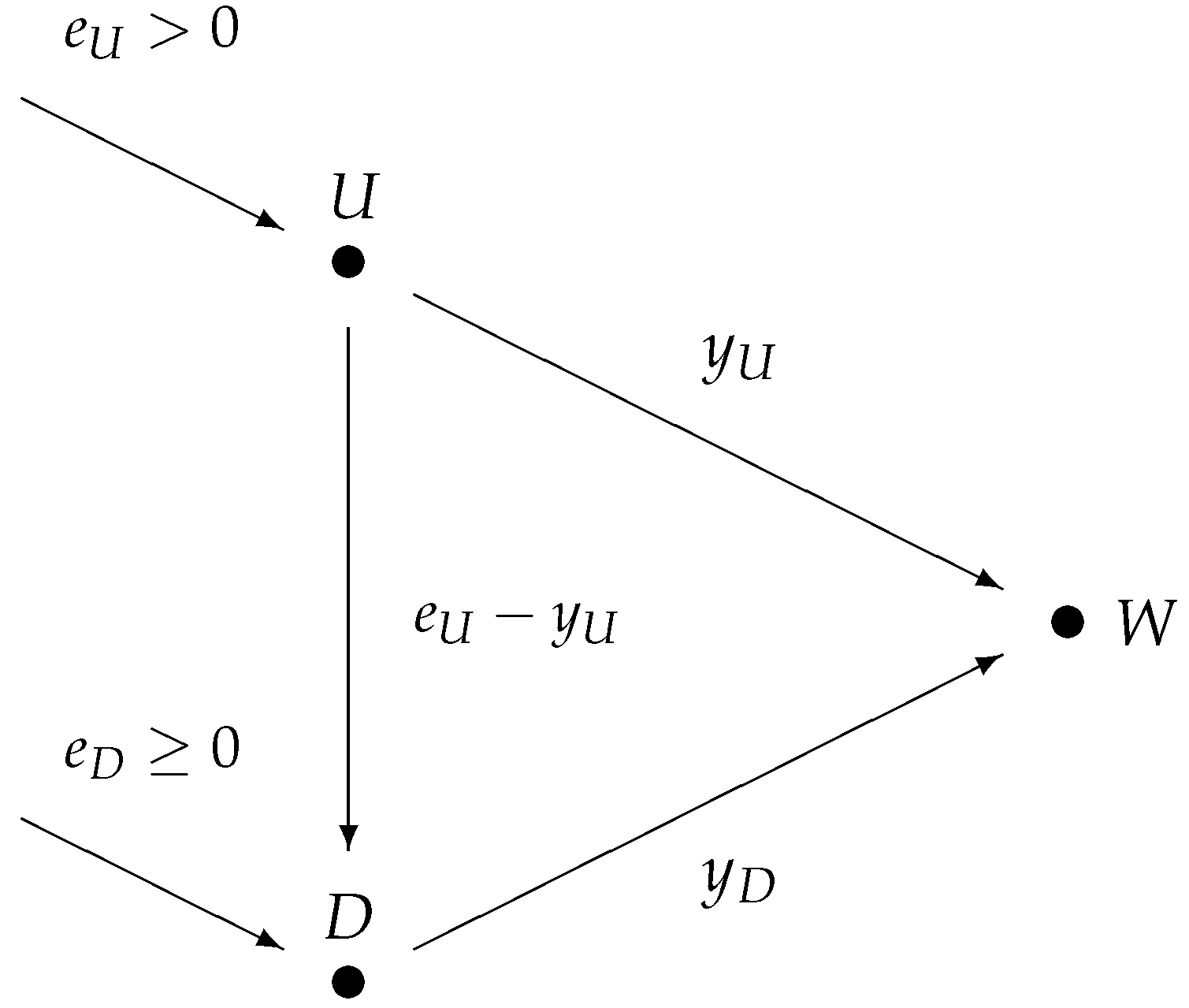
Each stretch is home to a water supplier, which we also label either U or D. Water suppliers extract water and both deliver it to the water market, which is denoted W. Water supplier U is restricted to accessing the upstream source exclusively, where it can extract a quantity of water denoted as for delivering it at the water market. Unused water flows downstream, where it augments the downstream’s water source, converting it into a total of . Downstream water supplier D can extract of water for the water market. Figure 1 illustrates these sources and water flows.
Water market W is modeled by a representative consumer who has a continuously differentiable, strictly concave benefit function such that benefit is impossible to attain without water and a positive marginal benefit for no or small amounts of water use, i.e., and . The determination of the willingness to pay for the combined quantity involves calculating the derivative of the benefit function. In quantity competition models, the willingness to pay is equal to the market-clearing price, which we denote as the price function rather than . Water scarcity arises when there is an inadequate combination of resources to achieve maximum benefit. As a result, water scarcity occurs when the willingness to pay, assuming full utilization of all sources, is positive. In our setting, scarcity is present for relatively small combined amounts . For the quadratic benefit function given by , we obtain the linear price function and water scarcity if .
The profit maximization objective applies to both suppliers. Supplier generates revenue . Additionally, the cost function associated with extracting and marketing the quantity is assumed to be non-decreasing and convex, represented by . Hence, the profit function for supplier i is expressed as .
The strategy profile given by the pair forms a SE if
It is important to note that the observable flow of water, which is given by , from upstream to downstream introduces the concept of time and sequential moves implicitly into the model. However, in our context, the social equilibrium concept remains independent of these notions and can be considered as a concept of simultaneous extractions.
In contrast, a Stackelberg approach recognizes that the observable flow of water is ultimately determined by upstream’s extraction, indicating a dynamic game. Consequently, as players in this dynamic setting, upstream moves first, followed by downstream. As a result, downstream’s strategy becomes a function that maps the combined resources available to downstream into an achievable extraction level. Formally, a strategy of downstream is a function . A strategy profile is given by the pair , where upstream chooses extraction and downstream the strategy . The strategy profile forms a SSE if
with the profit maximization of upstream given by
and with the profit maximization of downstream in every contingency given by
Any SSE in our setting can be characterized by applying backward induction.
3. Motivating Example
Our first contribution shows that the equilibrium characterization of Example 4.3 in Ansink and Houba (2012) [1] can be counterintuitive. First, we will briefly discuss their model and results.
In their Example 4.3, the market price function is given by , where there are no extraction costs and there is water scarcity, i.e., . The application of SE yields best-response functions for each supplier, denoted as , , which are given by
The first expression under each maximum refers to partial extraction and the second one to full extraction, which ensures feasible water extractions by each supplier. Solving all four cases, labeled (1)–(4), yields the SE extractions and their conditions as derived in Ansink and Houba (2012) [1], which we state here for convenience:4
In all cases, SE water extraction is at most . The full extraction of aggregate resources occurs in cases (1) and (3). Case (3) corresponds to the low upstream holding of partial extraction and the release of water downstream. Then, downstream fully extracts all of the combined resources. Moreover, in case (4), upstream releases water to downstream, and downstream partially extracts its available resources.
In our discussion, we will zoom in on cases (3) and (4) in more detail and simplify the situation to the extreme case in which upstream can be regarded as the monopolist of water in order to dramatize our argument, i.e., . Then, downstream fully relies on water released by upstream and can only extract water if upstream allows it to do so. For ease of discussion, we pick the number representing the boundary case of (3) and (4) with full extraction of available water. Furthermore, inflow to downstream is , the market price is , and each supplier makes a profit of .
To verify that this is an SE: given belief , supplier U solves with maximum and profit . Similar, given inflow and belief , supplier D solves with maximum and profit . In other words, given the equilibrium beliefs of equal extraction it is the best response for each supplier to extract half of the resource.
However, the SE outcome lacks the principle of backward induction. Upstream neglects that it controls inflow at downstream and that upstream can hold downstream at any level of inflow and even deprive downstream of water. If instead upstream would extract all of the available water, then downstream could not extract and supply a drop of water, while the market price would remain at and upstream’s profit would be doubled at . Clearly, the latter outcome in which upstream acts as a (ruthless) profit-maximizing monopolist seems a more intuitive outcome of strategic manipulation.
As an alternative solution concept, we propose SSE with upstream as the Stackelberg leader. This equilibrium concept introduces the backward induction logic. In our motivating example, the follower’s reaction function is given by for , and then the leader’s profit function is given by the increasing linear function on with full extraction as the boundary solution and maximal profit of , which is twice the SE profit. Hence, the analyses for cases (3) and (4) become similar, and the SSE outcome captures the strategic aspect of depriving downstream from water.
4. Stackelberg Social Equilibrium
A Stackelberg approach recognizes that the observable flow of water induces a dynamic setting in which upstream moves first, followed by downstream. As a consequence, downstream’s strategy becomes a function, and this changes the application of social equilibrium, which we have called Stackelberg social equilibrium in Section 2. In this section, we address two issues. First, we establish the existence of SSE in our setting under the same technical conditions under which SE exists in Ansink and Houba (2012) [1]. Second, we apply this concept to Example 4.3 of Ansink and Houba (2012) to derive the SSE.
A social equilibrium exists if all profit functions are strictly concave, as shown in Ansink and Houba (2012).5 Our next result establishes the existence of SSE under the same condition and provides a characterization.
Theorem 1.
If the profit function of supplier is strictly concave in , then a SSE exists in which
is a continuous function and maximizes the continuous function .
Proof.
The strict concavity of downstream’s profit function is sufficient to ensure that downstream’s maximization problem is a strictly convex program. By the Maximum Theorem, a single maximum exists, and it is a continuous function of all parameters, in particular . Therefore, the function is continuous in . After substitution, upstream’s profit function is continuous in on the compact interval . Hence, a profit maximum exists. The pair forms an SSE. □
We conclude this section with a demonstration of how to apply this result.
The Stackelberg Social Equilibrium of Example 4.3 of Ansink and Houba (2012)
Here, we revisit Example 4.3 of Ansink and Houba (2012) [1] and characterize the SSE. The functional forms are stated in Section 3, and all technical details are deferred to the Appendix A.
We solve for the SSE by applying backward induction. The follower’s profit-maximization problem is the same as in the SE for which the reaction function has been derived. The first expression under the minimum corresponds to the partial extraction of all combined resources by downstream, whereas the second expression expresses full extraction. It gives rise to three cases in upstream’s profit-maximization problem:
- The profit-maximizing quantity for downstream coincides with the upper bound on water extraction, i.e., . Then, upstream’s profit function is linear and increasing, and full extraction by upstream is profit maximizing.
- The profit-maximizing quantity for downstream lies below the upper bound on water extraction, i.e., . Then, upstream’s profit function is . Then, either extraction by upstream is profit maximizing whenever feasible, i.e., , or full extraction is profit maximizing if constrained, i.e., .
- Downstream will adopt the best response below the upper bound for low levels of extraction by upstream, while downstream chooses this upper bound for high levels of extraction by upstream. In this case, upstream’s profit-maximizing extraction is a mix of the first two cases, either full extraction or extraction.
Recall that the SE distinguishes the four distinct cases (1)–(4), where cases (3) and (4) correspond to upstream, which foregoes the ability to strategically manipulate its water release to downstream. In SSE there are only three cases, which we label (5)–(7). Their SSE extractions along the equilibrium path and their conditions are given by
Our cases (5) and (6) produce SSE extractions that are similar to the SE extractions of (1), respectively, (2). Partial SSE extractions by both suppliers are labeled case (7), and these differ from the SE extractions of case (4), which is similar to the classic result in the economics literature for Stackelberg and Cournot equilibrium. Furthermore, the SE extractions of case (3) are impossible in SSE. Additionally, the three SSE cases’ conditions differ from the four of SE. We forego a detailed analysis of the overlap of the areas under the conditions of SSE and SE.
In all cases, SSE water extraction is at most , and this upper bound is larger than the upper bound of in SE. This suggests an increase in aggregate extraction, which would be a deterioration of environmental issues such as river conservation. The reason for the increase in aggregate extraction is that by strategically releasing one unit of water less to downstream, the latter responds by reducing its extraction with one unit in case of full extraction and a half unit in case of partial extraction, resulting in a non-negative aggregate increase.
For the special case in which downstream fully relies on water released by upstream, case (6) is also excluded and downstream fully extracts all water whenever the source is sufficiently small, i.e., . For higher levels, both SSE extractions of upstream and downstream will be less than full extraction. At the boundary of (5) and (7), we have a nonrobust case of multiple equilibria.
5. Conclusions
An important source of friction in water markets is market power. Ansink and Houba (2012) analyze quantity competition among water suppliers along rivers with multiple sources and a single sink. Water suppliers extract water from the river and sell it to water users being constrained by the river flow, and they are connected to these users through a water delivery infrastructure. They define SE in terms of the simultaneous extractions of water and derive sufficient conditions for existence of SE. They also apply it to several examples.
In the duopoly water market case, Example 4.3 of Ansink and Houba (2012), we have argued that the presence of upstream and downstream suggests sequential moves and observable water releases. Furthermore, we have argued that a lack of backward induction logic may arise and that the upstream supplier foregoes profitable strategic manipulation of water to the downstream supplier. From a game theoretical point of view, incorporating both the notion of backward induction and strategy profiles with sequential moves, we propose the SSE concept. We prove the existence of SSE in duopoly water markets with an upstream–downstream river structure.
As a final result, we derive SSE in their Example 4.3. We show that the qualitative logic of three cases in SE, as derived in Ansink and Houba (2012), remains valid in SSE and that one of their cases for SE drops out: the criticized boundary case in our motivating example. The strategic manipulation of upstream’s water release to downstream leads to an upward pressure on aggregate extraction in SSE, comprising a deterioration of environmental issues such as river conservation. Our results establish that SSE is worth studying in water markets.
The concept of SSE in our setting is embedded in backward induction. For the more general case with multiple suppliers along a river with observable river flow, the direction of modifying the Markov perfect equilibrium, as defined in Maskin and Tirole (2001) [8], with river flow as the state variable seems a viable route forward to investigate sequential extractions and dynamic reasoning in the general framework of Ansink and Houba (2012).
Author Contributions
Writing—review and editing, H.H. and F.T. All authors have read and agreed to the published version of the manuscript.
Funding
Spanish Ministerio de Ciencia, Innovacion y Universidades and the European Union: ECO2016-75410-P, BES-2017-080192 and PID2019-105982GB-I00/AEI/10.13039/501100011033; Universitat Rovira i Virgili and the Generalitat de Catalunya: 2019PFR-URV-53.
Data Availability Statement
Not applicable.
Acknowledgments
We would like to thank Erik Ansink, Bernd Theilen, and the anonymous referees for their valuable comments and suggestions. Françeska acknowledges financial support from the Spanish Ministerio de Ciencia, Innovacion y Universidades, and the European Union under grants (ECO2016-75410-P, BES-2017-080192, and PID2019-105982GB-I00/AEI/10.13039/501100011033), and from the Universitat Rovira i Virgili and the Generalitat de Catalunya under the grant (2019PFR-URV-53).
Conflicts of Interest
The authors declare no conflict of interest.
Appendix A. Derivation of the SSE of Example 4.3 of Ansink and Houba (2012)
In Stackelberg duopoly models, the follower’s reaction function coincides with Cournot’s model best response function. This also applies to SE and SSE in the current setting and allows us to apply the results of Ansink and Houba (2012) [1]:
where the second expression under the maximum is D’s optimal water extraction under a non-binding upper bound on , i.e., , and the last expression is derived from a binding upper bound on water extraction, i.e., . Recall from Section 2 that water scarcity is defined as , which implies . Hence, we also have and a positive second expression under the maximum. To summarize, . Then, the minimum occurs for a binding upper bound , where the lower bound on can either exceed or be negative. The latter explains taking the minimum and maximum in the following reformulation:
For later use, we derive
- ⟺ ⟺ .
- ⟺ ⟺ .
- Otherwise, we have to deal with two subintervals of .
The Stackelberg leader’s profit function and upstream’s profit maximization problem can be rewritten as
We distinguish the three cases identified above.
- In this case, upstream solves . The linear function increases because of water scarcity, i.e., . Hence, we obtain boundary solution and upstream’s profit . Furthermore, and is downstream’s profit.
- Here, upstream solves . The maximum is given by , which implies two subcases. If , then yields upstream’s profit . Furthermore, , and is downstream’s profit. Similarly, if then , upstream’s profit is , , and downstream’s profit is .
- and Then, , and it partitions the interval into two subintervals. Both the linear and quadratic optimization under the maximum of upstream’s optimization problem should be considered. One difference with the previous cases is that has as its maximum. Note that ⟺ . After modifying previous arguments, we obtain: If , then generates profit for upstream and (because of water scarcity) with positive profit for downstream. If , then previous results imply generates profit for upstream and generates profit for downstream. Finally, the substitution of previous results yields the following upstream’s maximal profitBecause in this third main case and , we obtain the maximal profitand equilibrium path and if , while and if .
Summarizing the conditions of all cases, we have three important lines: , and . In -space; these lines intersect at and .
| 1 | |
| 2 | For background and further details of social equilibrium, see, e.g., Dasgupta and Maskin (2015) [7]. |
| 3 | There is an interesting analogy with the classic Stackelberg model. In that model, the leader setting the Cournot equilibrium quantity and the follower’s (constant) strategy to produce the Cournot equilibrium quantity irrespective of the leader’s quantity forms a Nash equilibrium. Obviously, this Nash equilibrium lacks backward induction and involves non-credible threats made by the follower. And it is the reason that the economic literature analyzes Stackelberg equilibrium instead. |
| 4 | The below-represented equations correspond to the equations (A)–(D) in [1]. |
| 5 | This reference also discusses in detail how these conditions restrict both benefit and cost functions. |
References
- Ansink, E.; Houba, H. Market power in water markets. J. Environ. Econ. Manag. 2012, 64, 237–252. [Google Scholar] [CrossRef] [Green Version]
- Ambec, S.; Ehlers, L. Sharing a river among satiable agents. Games Econ. Behav. 2008, 64, 35–50. [Google Scholar] [CrossRef]
- Chakravorty, U.; Hochman, E.; Umetsu, C.; Zilberman, D. Water allocation under distribution losses: Comparing alternative institutions. J. Econ. Dyn. Control 2009, 33, 463–476. [Google Scholar] [CrossRef] [Green Version]
- Holland, S. Privatization of water-resource development. Environ. Resour. Econ. 2006, 34, 291–315. [Google Scholar] [CrossRef]
- Tomori, F.; Ansink, E.; Houba, H.; Hagerty, N.; Bos, C.S. Market Power in California’s Water Market. SSRN Working Paper. 2021. Available online: https://papers.ssrn.com/abstract=3772167 (accessed on 25 June 2023).
- Debreu, G. A social equilibrium existence theorem. Proc. Natl. Acad. Sci. USA 1952, 38, 886–893. [Google Scholar] [CrossRef] [PubMed]
- Dasgupta, P.; Maskin, E. Debreu’s social equilibrium existence theorem. Proc. Natl. Acad. Sci. USA 2015, 112, 15769–15770. [Google Scholar] [CrossRef] [PubMed]
- Maskin, E.; Tirole, J. Markov perfect equilibrium. J. Econ. Theory 2001, 100, 191–219. [Google Scholar] [CrossRef] [Green Version]
Figure 1.
Water suppliers U and D along a river extract and deliver water to water market W.

Disclaimer/Publisher’s Note: The statements, opinions and data contained in all publications are solely those of the individual author(s) and contributor(s) and not of MDPI and/or the editor(s). MDPI and/or the editor(s) disclaim responsibility for any injury to people or property resulting from any ideas, methods, instructions or products referred to in the content. |
© 2023 by the authors. Licensee MDPI, Basel, Switzerland. This article is an open access article distributed under the terms and conditions of the Creative Commons Attribution (CC BY) license (https://creativecommons.org/licenses/by/4.0/).
Share and Cite
MDPI and ACS Style
Houba, H.; Tomori, F. Stackelberg Social Equilibrium in Water Markets. Games 2023, 14, 54. https://doi.org/10.3390/g14040054
AMA Style
Houba H, Tomori F. Stackelberg Social Equilibrium in Water Markets. Games. 2023; 14(4):54. https://doi.org/10.3390/g14040054
Chicago/Turabian StyleHouba, Harold, and Françeska Tomori. 2023. "Stackelberg Social Equilibrium in Water Markets" Games 14, no. 4: 54. https://doi.org/10.3390/g14040054
Note that from the first issue of 2016, this journal uses article numbers instead of page numbers. See further details here.