
Proposed Fuzzy-Stranded-Neural Network Model That Utilizes IoT Plant-Level Sensory Monitoring and Distributed Services for the Early Detection of Downy Mildew in Viticulture

Abstract
:1. Introduction
1.1. Related Work on Viticulture Downy Mildew Models
- Muller model is an empirical model based on temperature observations setting the infection occurrence when leaves are o 2 cm in diameter (E-L 9 development stage) and after heavy rain. According to this model, If the weather is dry (east wind), there is no risk of downy mildew, nor if the mean daily temperatures are below 12 °C or above 28 °C [10], the incubation period can be calculated in days. The actual daily add-ons to the sum based on the average daily temperature are provided by [22].
- Rule 3–10 is an empirical rule set by [23]. The rule states that infections initiate when the following conditions occur: Temperature, 10 °C, vine shoots of 10 cm long, and at least 10mm of rainfall over the last 24–48 h.
- Goidanich model. This model assumes initiation of primary infections at E-L 12 development stage, based on Rule 3–10. After infection, the percentage of daily development of incubation is calculated as Infection Risk Cycles (IRC), using an index value (Goidanich Index-GI) based on the average daily relative humidity and temperature until it reaches 100% [24]. An appropriate table of Goidanich’s model infection percentages is used for both primary and secondary infections [19]. Above 25°, IRC is constant. Furthermore, according to Puelles et al. evaluation [25], this model on Vitis vinifera usually delivers over-prediction infection blocks with very few matches to field observations. Nevertheless, this differs from the research in northwestern Spain provided by [26].
- EPI model. This model, developed by Stryzik et al. [27], uses an EPI index metric that represents the pathogen potential infection energy for primary infections and the kinetic energy for secondary infections. For primary infections, it utilizes a set of equations that consider monthly rainfall and temperature, the number of days with rain per month, and the rainfall during the last ten days. For secondary infections, the model takes into account inputs of temperature, relative humidity, and relative humidity at night [9,28]. Potential infection energy is calculated using Equation (1) from October until January [27].where the value k is 1.2 in October, 1 in November, and 0.8 for the rest of the months (until March), is the daily rainfall, is the mean monthly rainfall, the mean daily temperature, the mean monthly temperature, cumulative rainfall the last ten days, , number of monthly rainy days and number of rainy days the last ten days [27].Equation (2) gives the kinetic energy of the model calculated from April until September and corresponds to primary and secondary infections since the model assumes that oospore maturity is reached by the 31st of March [27].where is the average relative humidity at night, and is the average relative daily humidity, the average daily temperature, and the monthly average temperature. Finally, the EPI index value is calculated based on Equation (3) [27].From October until the end of March, the value of the EPI metric is an estimate of oospore maturation, where the first infection occurs when EPI > −10, while the EPI increases for three consecutive days [27].
- Downy Mildew foreCast is a model that tries to provide primary and secondary infection predictions. It uses a probabilistic normal distribution for primary infections using Equation (4) [29]where mean and standard deviation parameters are calculated by parameter , which is the cumulative rainfall effect at the end of January according to Equation (5) [29].where is the mean monthly rainfall, is the mean standard deviation of monthly rainfall, are the total monthly rainy days and is the daily rainfall. Primary infections initiate when the daily probability outcome reaches 3%. From this day forth, secondary infections are calculated as mentioned at [29]. It is considered that infections occur when rainfall is at least 2 mm and T ≤ 11 °C, while for seven up to 22 days after the beginning of oospore germinations [29].
- UCSC model was developed by Rossi et al. [8]. The model simulates, using a granularity time step of one hour, the entire process, starting from oospore maturation and germinations to zoospore discharge and dispersal and finally to secondary infection cycles [9]. The model uses sensory measurements of temperature, relative humidity, leaf wetness, and rainfall as inputs. Briefly, the model calculates the time when the first break of the oospore’s dormancy occurs (about the 1st of January), as well as the primary and secondary infection progress, by calculating the Relative Incidence of Infection (RII) metric value [2,4,8]. The metrics used by the model are shown in Table 1 [8].Furthermore, Table 1 at [9], shows the model input parameters for oospore maturation and oospore-zoospore germination stages.
- UR model. This is a Goidanich-table-based model alternative that tries to address both primary and secondary infections [25]. According to this model, oospore maturation in winter is reached if the value of a cumulative temperatures sum reaches 140–160 °C. This sum is calculated using mean daily temperatures (), starting from the 1st of January, and using the following Equation (6) [30,31].If oospore maturation is reached, then oospore germination occurs, providing primary sporangia either when mean relative humidity > 80 and mean temperature > 8 for an 8-h window or when mean precipitation occurs more than 5 mm ( > 5) for the last 48 h. The first dispersion of zoospores is reached after oospore germination, when mean rainfall RF > 3 mm and > 8 for a 6 h interval (a modified 3–10 Rule). Then primary infections occur, if Degree hours Dh > 50, calculated based on Equation (7) [30,31].where is the hourly temperature (hour ) and is the hourly relative humidity. Secondary infections are calculated using the Goidanich table index. To achieve sporulation for secondary infections, two conditions needed to be met: % or temperatures between 12 °C and 29 °C for at least 4 h at night [25]. Additionally, the model considers that exposure to more than 6 h above 30 °C results in the death of oospores, both for primary and secondary infections [32].
- Milvit Model. Developed by the French Plant Protection Service in the late 80s. It is a potato downy mildew simulated model, a pathogen with similar pathogen characteristics to P. viticola [33]. As mentioned by Magnien et al. [33], it uses temperature and relative humidity, four stages of the pathogen cycle. It is also supported by a DSS system. Nevertheless, this model is not taken into account since it is not targeting the phenological characteristics of V. vinifera and since, as mentioned by Puelles et al. experimentation [25], it has shown both over-prediction and under-prediction infection blocks compared to field observations.
- Vitimeteo—Plasmopara is a mechanistic model based on experimental observations, created by Bleyer et al. [34]. This model tries to predict both primary and secondary infections. The main model components are three stages: (1) Maturation oospores stage, (2) primary, and (3) secondary infections. Regarding (1) and (2) the UR model is used. However, secondary infections are calculated using mean temperature degree hours Dh > 50, if 3 < < 29, and if hourly relative humidity > 95% [34].

| Environmental Description | Temperature (T °C) | Humidity (%) | Daily Rainfall () | FGI () |
|---|---|---|---|---|
| warm and wet | 13 < T ≤ 28 | 70 < RH ≤ 100 | RF ≥ 5 | 1 |
| warm and partly wet | 13 < T ≤ 28 | 70 < RH ≤ 95 | 0 < RF < 5 | 0.6 |
| warm and dry | 13 < T ≤ 28 | 70 ≤ RH ≤ 95 | RF = 0 | 0.4 |
| warm and very dry | 13 < T ≤ 28 | RH < 70 | RF = 0 | 0.1 |
| cold and wet | 0 < T ≤ 13 | RH < 70 < RH ≤ 100 | RF ≥ 5 | 0.8 |
| cold and partly wet | 0 < T ≤ 13 | 70 < RH ≤ 95 | 0 < RF < 5 | 0.48 |
| cold and dry | 0 < T ≤ 13 | 70 ≤ RH ≤ 95 | RF = 0 | 0.32 |
| cold and very dry | 0 < T ≤ 13 | RH < 70 | RF = 0 | 0.08 |
1.2. Conclusions of Downy Mildew Models Examination
- Unlike the experimental varieties and conditions examined, all models fail to cope with the phenomenon’s evolution over attributes such as different environmental conditions, variety, and vine ages. No mechanistic model can be set as a catholic-holistic model due to the non-uniformity of the attributes described above, with the exception of some conservative empirical generic rules (for example, Rule 3–10).
- Mechanistic models trying to time the downy mildew disease process accurately can easily lead to erroneous calculations of significant offsets if the coefficients or variable parameters used do not match the examined environmental conditions that have been experimentally calculated (miscalibration). That is why, in several cases, empirical models can outperform mechanistic ones and can provide much more safe-ground predictions.
- Most mechanistic models target on-time evolution modeling of downy mildew and do not excerpt a decision suggestion required by Decision Support Systems. They are leaving such decisions to the non-expert’s eye. Such as precision viticulture practices (for example, vine leaves removal) or pesticide appliances and analogies (such as Bordeaux mixture products appliance).
- All models, specifically mechanistic ones (of higher sensory measurements, high granularity dependency), utilize meteorological station measurements. Such measurements are kept at best in hourly mean intervals. Furthermore, meteorological stations located at high elevation grounds, with 5–20 km radius coverage, servicing large areas of nonuniform terrestrial fields, cannot cope with the condition extrapolates. Due to this type of exploited input, they can provide only best-effort forecasts of significant field-level disease variations, thus leading to over-pesticide field uses in many cases.
- Downy mildew mechanistic models are trying to provide time-frames and thresholds for primary and secondary infections corresponding to large areas of different conditions. Because their inputs are in sparse hourly periods and are of single points of reference (single meteorological stations), without experimental calibrations of their coefficients, on field vine clusters, or on the monitored field areas, such models will consistently be outperformed by empirical ones.
1.3. Downy Mildew Forecasting DSS Systems
- Meteo Station Data: Weather the DSS system also receives data inputs from meteorological stations via specifically designed protocols or interfaces. Meteorological stations.
- IoT Plant level Monitoring: Whether the DSS system acquires plant-level information using IoT sensors.
- Auto location tracking: Whether the DSS system can track its data input sources using GPS receivers (locality).
- data acquisition: The schema form that the DSS logging service stores the sensory data measurements, that can sustain big data records of different measurements-attributes over time as mentioned at [62].
- Low-cost data transmissions: Covers the low-power data transponder specifications of DSS systems that use nodes capable of plant-level monitoring. Such transponders are RF-based, NBIoT, LoRa, LoRaWAN, Wi-Fi, ZigBee, or BLE/Bluetooth, which maintain low energy footprints, in contrast to the power consumption of GSM GPRS/3G/4G-LTE transponders [63]. This performance characteristic also considers the required network provider costs per node, especially for technologies such as NBIoT and GSM/GPRS/3G/4G.
- ReST API: If the DSS system includes appropriate SDK API to fetch data measurements or forecasts by clients using HTTP/UDP/CoAP/MQTT or custom protocol requests [64].
- Interfaces: Type of accessible user interfaces offered by the DSS system (Web, Mobile App, Custom Application UI)
- OpenSource components: If the DSS utilizes open-source components SDKs or libraries
- Installation-Maintenance efforts: Whether the DSS system and its end vine-level nodes are easy to Install and scale, and the farmers’ minimum or no maintenance efforts are required.
2. Materials and Methods
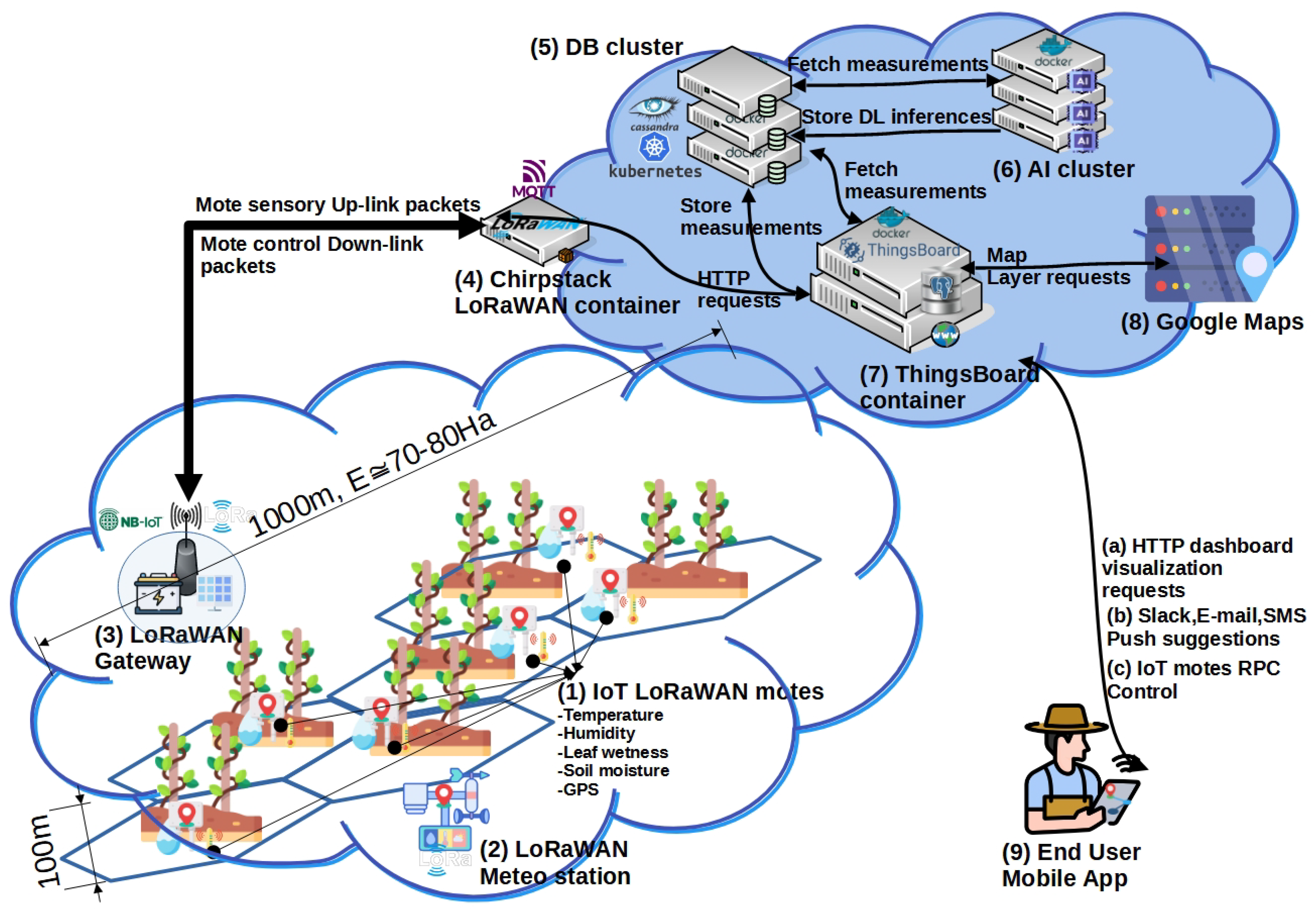
2.1. Proposed High-Level System Architecture
- Vine field device components: These include: 1. the IoT mote devices equipped with GPS receivers and a LoRaWAN transponder, acquiring field sensory measurements (see Figure 1, (1)), such as temperature, humidity, leaf wetness and soil moisture, and 2. the LoRaWAN meteorological stations (see Figure 1, (2)), which include a GPS receiver, LoRaWAN transponder, pressure, temperature, humidity, wind speed, direction sensors, and a rain gauge. In each viticulture field, the farmers place the IoT motes to measure plant-level sensory parameters of different mote profiles, for instance, temperature and humidity, according to our downy mildew experimentation. The suggested coverage area for an IoT mote is more of a regular hexagon with either height () or width (), where a = 100 m. That is, a coverage area of per IoT mode device. The authors set the maximum coverage area for an IoT mode for vine-level monitoring up to 1 Ha. Usually, IoT motes are placed according to the following rules: (1) If there is a significant elevation difference between two points in a field more than 1 m, (2) If there is a slope of more than 20°, offering different soil drainage, and (3) if there is tree coverage near the field contributing to a significant reduction of at least 2 h of sun throughout the day concerning the rest of the viticulture field. LoRaWAN meteorological stations are usually installed in pinpointed locations based on the ground morphological characteristics, covering field areas of 70–80 Ha. The field components also include the LoRaWAN gateway, which acts as a sensory measurements concentration and thinsAI data forwarding point to the thingsAI LoRa Server [54].The sensory motes transmit measurements of temperature and humidity every period intervals. These intervals can be programmable over the air by the farmers via ThingsBoard panels (with a minimum value of every 1 min and a maximum value of 4 h), using Class A LoRaWAN data reception windows RX1, RX2 [71]. The motes also transmit GPS location LoRaWAN frames that can be set to every 8–48 h. The same applies to the LoRaWAN meteorological stations. The LoRaWAN meteorological station coverage area may extend more than 70–80 Ha and is used to capture meteorological measurements that accurately correspond to the included viticulture fields vine-clima. There is no need for vine-level measurements of wind speed, direction, or rain since their variations can be accurately captured using at least 1 km meteo-stations dense coverage. LoRaWAN meteorological stations are autonomous battery-operated devices with a mean power consumption of 1.8–3 W, transmitting measurements per-minute intervals via class A LoRaWAN protocol to the LoraWAN gateways. For the meteorological stations, different communication technologies can also be used, such as NBIoT UMTS(3G) or Wi-Fi, in order to transmit measurements to the thingsAI cloud infrastructure directly through the ThingsBoard container (see Figure 1, (7) ThingsBoard AS) bypassing the LoRaWAN application server (see Figure 1, (4) LoRaWAN AS).The thingsAI system field components utilize a dense grid of GPS-equipped IoT motes (see Figure 1, (1)) and a sparse grid of GPS-equipped LoRaWAN meteorological stations (see Figure 1, (2)) to provide sensory measurements at vine level. All motes (see Figure 1, (3)) transmit their GPS location using LoRaWAN frames via the gateway. The gateways use two communication technologies (NBIoT and LoRaWAN) deliberately made to minimize telecommunication provider costs. NBIoT transponders could have been used instead of LoRaWAN for end-device data transmissions (motes and meteorological stations). Nevertheless, such a technological alternative enforces a per mote SIM card annual communication fee for the farmers. Depending on the number of IoT motes used, the provider fees could reach up to 2–4€/device/month. Instead, the authors propose using the LoRaWAN communication as a free long-range narrow-band alternative of a single connection point with one cellular telecommunications link at the gateway bridge. Since the LoRaWAN coverage extends from 5–12 km, a single gateway may cover a significant portion of a huge cultivation area [72].LoRaWAN gateways (see Figure 1, (3) LoRaWAN gateways), are responsible for forwarding IoT mote measurement frames to the LoRaWAN network service and, therefore, to the application server (Figure 1, (4) LoRaWAN container) [69]. This is achieved by maintaining Internet connectivity via a cellular NBIoT network provider at the gateway level. The LoRaWAN gateways are autonomous devices of continuous operation, with a mean power consumption of 5–6 W, because they are operating simultaneously two different transponders: an NBIoT(GR-800MHz/B20) UART transponder of a 10 MHz/channel bandwidth and a LoRaWAN (EU:863–870 MHz) concentrator board of a 125 KHz/channel bandwidth. In areas where the B20 band is unavailable, the UMTS B21 band of 2100 MHz is used with higher channel bandwidths of 20 MHz/channel. All IoT motes and meteorological stations join the LoRa server using Over The Air Activation (OTAA). All IoT motes and meteorological stations have ADR LoRaWAN capabilities enabled. All motes transmit sensory data via the available LoRaWAN channels 1–8 and receive downlink windows RX1 via the data transmitting channel and RX2 at 869.5 MHz [71].
- Cloud Components: These are mainly docker containers that reside in a single or multiple cloud Virtual Machine instances [69]. The thingsAI cloud components as shown in Figure 1, include the: 4. LoRaWAN container of the chirpstack LoRa server [73], the 5. Cassandra No-SQL clustered database [74], for storing sensory measurements, the 6. AI containers running deep learning training and classification, prediction tasks, and the 7. ThingsBoard Application Server (AS), platform container capable of providing visualization outputs, motes control, and suggestions-alerts to the end users.The chirpstack LoRa server [73] (see Figure 1, (4)), is an open-source network and application server capable of receiving encrypted AES-128 data transmissions from the LoRaWAN gateways. Upon data validation and decryption, the data are pushed to the Chirpstack container mosquito Message Queue Telemetry Transport (MQTT) service [75]. Then, the appropriate data logging agent using MQTT subscribe mechanism acquires the sensory measurements and submits them as HTTP post-device telemetry requests, depending on the LoRaWAN mote device ID, to the ThingsBoard Application server [76].The ThingsBoard AS (see Figure 1, (7) ThingsBoard AS) is responsible for controlling all thingsAI devices (motes and meteorological stations) and device attributes at the application level, as well as storing the per-device sensory measurements and GPS locations at the Cassandra distributed Database cluster [74] (see Figure 1, (5)). In the ThingsBoard AS container reside the data logging service, the geo-location module, acquiring Google Map layers information (see Figure 1, (8)), the RPC motes control service, and notification services described in detail in Section 2.3.Finally, the thingsAI cluster (see Figure 1, (6)), described in Section 2.3, is a set of docker containers where the Deep Learning models, models’ training agents and inference services are instantiated, providing classifications and predictions.
2.2. ThingsAI IoT Motes and Stations
- At least one sensory mote must exist in a rectangular area of 100 × 100 m (1 Hectare) called the maximum partitioning area
- If required due to elevation differences >0.8–2 m, the maximum partitioning area can be clustered into two or more areas where different motes are placed (vertical partitioning)
- If significant variances inside the maximum partitioning area occur with respect to direct hourly solar radiation measured daily at W/m due to shadowing caused by nearby tree clusters or other environmental factors, such as nearby water streams. Such calculations preferably take into account either monthly mean hourly differences of Vapor Pressure Deficit (VPD) in kPa for months May–Aug or reference evapotranspiration , in mm, based on PenMan-Monteith equations [77], as a cumulative sum for months May-August. At least one monthly variance of VPD , or a yearly evapotranspiration difference of 30 mm/y, taking into account as a full year the months of May-Aug, denote an area partitioning into two different regular hexagon areas, whose centers are the two variation points of either VPD or .
- Either a COTS 32 bit ESP32 cortex-M3 MPU 32 MHz, of 128 KB Flash, 16 KB or RAM and 4 KB of EEPROM and LoRaWAN onboard transponder that periodically collects and transmits sensory measurements using LoRaWAN frames [78], or Seeduino LoRaWAN RHF76-052AM board with the ATSAMD 48 MHz CPU and an onboard GPS receiver [79] can be used.
- DHT22 temperature and humidity sensor. Other sensors, such as leaf-wetness and soil moisture sensors, can also be attached.
- LoRaWAN 14 dBm, 868 MHz transponder supporting class A LoRaWAN protocol.
- a Ublox NEO-6M GPS on board UART receiver.
- 3.6 V, 8000 mA Lithium replaceable battery case connected with the board using a JST2.0 cable.
- Plastic IP67 casing.
- GPS antenna.
- LoRAWAN antenna.
2.3. ThingsAI LoRaWAN Application Protocols and Cloud Services
2.4. ThingsAI Downy Mildew Model
3. Experimental Scenario
3.1. Training Model Evaluation
3.2. Trained Model Experimentation
3.3. Scenario I: Model Experimentation under Normal Conditions
3.4. Scenario II: Model Experimentation under Downy Mildew Outbursts
4. Conclusions
Author Contributions
Funding
Data Availability Statement
Conflicts of Interest
Abbreviations
| ACK | Acknowledgment frame |
| AS | Application Server |
| COTS | Component Out of The Self |
| DSS | Decision Support Systems |
| EEPROM | Electrically Erasable Programmable Read Only Memory |
| GI | Goidanich Index value |
| GPS | Global Positioning System |
| Ha | Hectars, Area Unit of measurement |
| I2C | Inter-Integrated Circuit synchronous digital communication protocol |
| KPI | Key Performance Indicators |
| NBIoT | Narrow Band Internet of Things |
| NMEA | National Marine Electronics Association positioning standards |
| NN | Fully Connected Neural Networks |
| OGC | Open Geospatial Consortium |
| OTAA | Over The Air Activation |
| SDK | Software Development Kit |
| SOS | Sensor Observation Services |
| SPI | Synchronous Peripheral Interface, serial communication protocol |
| Str | Stremmata area Unit of measurement equal to 1000 m2 = 0.1 Ha |
| SVM | Support Vector Machines |
| UART | Universal asynchronous Receiver-Transmitter |
| Vitis Vinifera | Common grape vine varieties in EU |
| VPD | Vapor Pressure Deficit metric |
| VU | Vine Units |
| P. viticola | Plasmopara Viticola, downy mildew |
References
- Fontaine, M.C.; Labbé, F.; Dussert, Y.; Delière, L.; Richart-Cervera, S.; Giraud, T.; Delmotte, F. Europe as a bridgehead in the worldwide invasion history of grapevine downy mildew, Plasmopara viticola. Curr. Biol. 2021, 31, 2155–2166. [Google Scholar] [CrossRef] [PubMed]
- Velasquez-Camacho, L.; Otero, M.; Basile, B.; Pijuan, J.; Corrado, G. Current Trends and Perspectives on Predictive Models for Mildew Diseases in Vineyards. Microorganisms 2022, 11, 73. [Google Scholar] [CrossRef] [PubMed]
- Bove, F.; Savary, S.; Willocquet, L.; Rossi, V. Designing a modelling structure for the grapevine downy mildew pathosystem. Eur. J. Plant Pathol. 2020, 157, 251–268. [Google Scholar] [CrossRef]
- Rossi, V.; Caffi, T.; Gobbin, D. Contribution of molecular studies to botanical epidemiology and disease modelling: Grapevine downy mildew as a case-study. Eur. J. Plant Pathol. 2013, 135, 641–654. [Google Scholar] [CrossRef]
- Pearce, I.; Coombe, B. Grapevine Phenology Revised version of Grapevine growth stages. The modified E-L system. In Viticulture Resources, 2nd ed.; Winetitles: Broadview, SA, Australia, 2004; Volume 1. [Google Scholar]
- Caffi, T.; Gilardi, G.; Monchiero, M.; Rossi, V. Production and release of asexual sporangia in Plasmopara viticola. Phytopathology 2013, 103, 64–73. [Google Scholar] [CrossRef]
- Bove, F.; Savary, S.; Willocquet, L.; Rossi, V. Simulation of potential epidemics of downy mildew of grapevine in different scenarios of disease conduciveness. Eur. J. Plant Pathol. 2020, 158, 599–614. [Google Scholar] [CrossRef]
- Rossi, V.; Caffi, T.; Bugiani, R.; Spanna, F.; Valle, D.D. Estimating the germination dynamics of Plasmopara viticola oospores using hydro-thermal time. Plant Pathol. 2008, 57, 216–226. [Google Scholar] [CrossRef]
- Caffi, T.; Rossi, V.; Cossu, A.; Fronteddu, F. Empirical vs. mechanistic models for primary infections of Plasmopara viticola. EPPO Bull. 2007, 37, 261–271. [Google Scholar] [CrossRef]
- Müller, K. Die biologischen Grundlagen für die Peronosporabekämpfung nach der Inkubationskalender-Methode. Z. FüR Pflanzenkrankh. (Pflanzenpathol.) Pflanzenschutz 1936, 46, 104–108. [Google Scholar]
- Lalancette, N.; Ellis, M.A.; Madden, L.V. Development of an infection efficiency model for Plasmopara viticola on American grape based on temperature and duration of leaf wetness. Phytopathology 1988, 78, 794–800. [Google Scholar] [CrossRef]
- Zachos, D. Recherches sur la biologie et l’épidémiologie du mildiou de la vigne en Grèce. Ann. Inst. Phytopathol. Benaki 1959, 2, 193–335. [Google Scholar]
- Peladarinos, N.; Piromalis, D.; Cheimaras, V.; Tserepas, E.; Munteanu, R.A.; Papageorgas, P. Enhancing Smart Agriculture by Implementing Digital Twins: A Comprehensive Review. Sensors 2023, 23, 7128. [Google Scholar] [CrossRef]
- Ferro, M.V.; Catania, P. Technologies and Innovative Methods for Precision Viticulture: A Comprehensive Review. Horticulturae 2023, 9, 399. [Google Scholar] [CrossRef]
- Kontogiannis, S.; Asiminidis, C. A Proposed Low-Cost Viticulture Stress Framework for Table Grape Varieties. IoT 2020, 1, 337–359. [Google Scholar] [CrossRef]
- Trilles, S.; Torres-Sospedra, J.; Belmonte, O.; Zarazaga-Soria, F.J.; Gonzalez-Perez, A.; Huerta, J. Development of an open sensorized platform in a smart agriculture context: A vineyard support system for monitoring mildew disease. Sustain. Comput. Inform. Syst. 2020, 28, 100309. [Google Scholar] [CrossRef]
- Hnatiuc, M.; Ghita, S.; Alpetri, D.; Ranca, A.; Artem, V.; Dina, I.; Cosma, M.; Abed Mohammed, M. Intelligent Grapevine Disease Detection Using IoT Sensor Network. Bioengineering 2023, 10, 1021. [Google Scholar] [CrossRef]
- Mezei, I.; Lukić, M.; Berbakov, L.; Pavković, B.; Radovanović, B. Grapevine Downy Mildew Warning System Based on NB-IoT and Energy Harvesting Technology. Electronics 2022, 11, 356. [Google Scholar] [CrossRef]
- Pérez-Expósito, J.P.; Fernández-Caramés, T.M.; Fraga-Lamas, P.; Castedo, L. VineSens: An Eco-Smart Decision-Support Viticulture System. Sensors 2017, 17, 465. [Google Scholar] [CrossRef]
- Kasapakis, I. ZenAgro Company LLC. 2021. Available online: https://zenagropc.com/ (accessed on 1 February 2021).
- Mian, G.; Buso, E.; Tonon, M. Decision Support Systems for Downy Mildew (Plasmopara viticola) Control in Grapevine: Short Comparison Review. Asian Res. J. Agric. 2021, 14, 12–20. [Google Scholar] [CrossRef]
- Ostojić, Z. Priručnik Izveštajne i Prognozne službe zaštite Poljoprivrednih Kultura; Savez Drustava Za Zastitu Bilja: Belgrade, Yugoslavia, 1983. [Google Scholar]
- Baldacci, E. Epifitie di Plasmopara viticola (1941–46) nell’Oltrepó Pavese ed adozione del calendario di incubazione come strumento di lotta. Atti Ist. Bot. Lab. Crittogam. 1947, 8, 45–85. [Google Scholar]
- Goidanich, G.; Casarini, B.; Foschi, S. Lotta antiparassitaria e calendario dei trattamenti in viticoltura. Giornale di Agricoltura 1957, 13, 11–14. [Google Scholar]
- Puelles, M.; Arbizu-Milagro, J.; Castillo-Ruiz, F.J.; Peña, J.M. Predictive models for grape downy mildew (Plasmopara viticola) as a decision support system in Mediterranean conditions. Crop Prot. 2024, 175, 106450. [Google Scholar] [CrossRef]
- Fernández-González, M.; Piña-Rey, A.; González-Fernández, E.; Aira, M.J.; Rodríguez-Rajo, F.J. First assessment of Goidanich Index and aerobiological data for Plasmopara viticola infection risk management in north-west Spain. J. Agric. Sci. 2019, 157, 129–139. [Google Scholar] [CrossRef]
- Stryzik, S. Modéle d’état potentiel d’infection: Application a Plasmopara viticola. In Association de Coordination Technique Agricole; Maison Nationale des Eleveurs: Paris, France, 1983; pp. 1–46. [Google Scholar]
- Sanna, F.; Cossu, A.; Roggero, G.; Bellagarda, S.; Deboli, R.; Merlone, A. Evaluation of EPI forecasting model with inclusion of uncertainty in input value and traceable calibration. In Proceedings of the 17th Conference Convegno Nazionale di Agrometeorologia—AIAM, Rome, Italy, 10–12 June 2014; pp. 61–63. [Google Scholar]
- Park, E.; Seem, R.; Gadowry, D.; Pearson, R. DMCast: A prediction model for grape downy mildew development. Viticutural Enol. Sci. 1997, 52, 182–189. [Google Scholar]
- Gehmann, K.; Staudt, G.; Grossmann, F. Der Einfluß der Temperatur auf die Oosporenbildung von Plasmopara viticola / The influence of temperature on oospore formation of Plasmopara viticola. Z. FüR Pflanzenkrankh. Pflanzenschutz/ J. Plant Dis. Prot. 1987, 94, 230–234. [Google Scholar]
- Dubuis, P.H.; Viret, O.; Bloesch, B.; Fabre, A.L.; Naef, A.; Bleyer, G.; Kassemeyer, H.H.; Krause, R. Lutte contre le mildiou de la vigne avec le modèle VitiMeteo-Plasmopara. Rev. Suisse Vitic. Arboric. Hortic. 2012, 44, 192. [Google Scholar]
- Blaeser, M.; Weltzien, H. Epidemiologische Studien an Plasmopara viticola zur Verbesserung der Spritzterminbestimmung/Epidemiological studies to improve the control of grapevine downy mildew (Plasmopara viticola). Z. Für Pflanzenkrankh. Pflanzenschutz/J. Plant Dis. Prot. 1979, 86, 489–498. [Google Scholar]
- Magnien, C.; Jacquin, D.; Muckensturm, N.; Guillemard, P. MILVIT: A descriptive quantitative model for the asexual phase of grapevine downy mildew. IOBC/WPRS Bull. 1991, 21, 451–459. [Google Scholar]
- Bleyer, G.; Kassemeyer, H.H.; Krause, R.; Viret, O.; Siegfried, W. VitiMeteo Plasmopara—Prognosemodell zur Bekämpfung von Plasmopara viticola (Rebenperonospora) im Weinbau. Gesunde Pflanz. 2008, 60, 91–100. [Google Scholar] [CrossRef]
- Savary, S.; Nelson, A.D.; Djurle, A.; Esker, P.D.; Sparks, A.; Amorim, L.; Bergamin Filho, A.; Caffi, T.; Castilla, N.; Garrett, K.; et al. Concepts, approaches, and avenues for modelling crop health and crop losses. Eur. J. Agron. 2018, 100, 4–18. [Google Scholar] [CrossRef]
- Reuveni, M. Relationships between Leaf Age, Peroxidase and β-1,3-Glucanase Activity, and Resistance to Downy Mildew in Grapevines. J. Phytopathol. 1998, 146, 525–530. [Google Scholar] [CrossRef]
- Salotti, I.; Bove, F.; Ji, T.; Rossi, V. Information on disease resistance patterns of grape varieties may improve disease management. Front. Plant Sci. 2022, 13, 1017658. [Google Scholar] [CrossRef] [PubMed]
- Lalancette, N. Estimating Infection Efficiency of Plasmopara viticola on Grape. Plant Dis. 1987, 71, 981. [Google Scholar] [CrossRef]
- Gessler, C.; Pertot, I.; Perazzolli, M. Plasmopara viticola: A review of knowledge on downy mildew of grapevine and effective disease management. Phytopathol. Mediterr. 2011, 50, 3–44. [Google Scholar]
- Damalas, C.A.; Eleftherohorinos, I.G. Pesticide exposure, safety issues, and risk assessment indicators. Int. J. Environ. Res. Public Health 2011, 8, 1402–1419. [Google Scholar] [CrossRef] [PubMed]
- Fungicide Resistance Action Committee. Fungal Control Agents Sorted by Cross-Resistance Pattern Andmode of Action. 2023. Available online: https://www.frac.info/docs/default-source/publications/frac-code-list/frac-code-list-2023—final.pdf (accessed on 1 November 2023).
- Wyenandt, A. Understanding Phenylamide (FRAC Group 4) Fungicides. 2020. Available online: https://plant-pest-advisory.rutgers.edu/understanding-phenylamide-frac-group-4-fungicides/ (accessed on 1 September 2022).
- Sharma, N.; Nasrollahiazar, E.; Miles, L.; Miles, T. Michigan Grape Facts: Managing Grapevine Downy Mildew. Grapes 2023. Available online: https://www.canr.msu.edu/resources/michigan-grape-facts-managing-grapevine-downy-mildew (accessed on 1 November 2023).
- Chen, M.; Brun, F.; Raynal, M.; Makowski, D. Forecasting severe grape downy mildew attacks using machine learning. PLoS ONE 2020, 15, e0230254. [Google Scholar] [CrossRef] [PubMed]
- Léger, B.; Naud, O.; Bellon-Maurel, V.; Clerjeau, M.; Delière, L.; Cartolaro, P.; Delbac, L. GrapeMilDeWS: A Formally Designed Integrated Pest Management Decision Process Against Grapevine Powdery and Downy Mildews. In Decision Support Systems in Agriculture, Food and the Environment: Trends, Applications and Advances; IGI Global: Hershey, PA, USA, 2010; pp. 246–269. [Google Scholar] [CrossRef]
- Rossi, V.; Salinari, F.; Poni, S.; Caffi, T.; Bettati, T. Addressing the implementation problem in agricultural decision support systems: The example of vite.net®. Comput. Electron. Agric. 2014, 100, 88–99. [Google Scholar] [CrossRef]
- Dubuis, P.H.; Bleyer, G.; Krause, R.; Viret, O.; Fabre, A.L.; Werder, M.; Naef, A.; Breuer, M.; Gindro, K. VitiMeteo and Agrometeo: Two platforms for plant protection management based on an international collaboration. BIO Web Conf. 2019, 15, 01036. [Google Scholar] [CrossRef]
- Davy, A.; Raynal, M.; Vergnes, M.; Debord, C.; Codis, S.; Naud, O.; Delière, L.; Fermaud, M.; Roudet, J.; Metral, R.; et al. Decitrait®: Un OAD pour la protection de la vigne. Innov. Agron. 2020, 79, 89–99. [Google Scholar]
- Koufos, G.C.; Mavromatis, T.; Koundouras, S.; Jones, G.V. Response of viticulture-related climatic indices and zoning to historical and future climate conditions in Greece. Int. J. Climatol. 2018, 38, 2097–2111. [Google Scholar] [CrossRef]
- Zinas, N.; Kontogiannis, S.; Kokkonis, G.; Pikridas, C. A novel microclimate forecasting system architecture integrating GPS measurements and meteorological-sensor data. In Proceedings of the 6th Balkan Conference in Informatics, BCI’13, Thessaloniki, Greece, 19–21 September 2013; pp. 82–88. [Google Scholar] [CrossRef]
- Trilles, S.; Lujan, A.; Belmonte, O.; Montoliu, R.; Torres Sospedra, J.; Huerta, J. SEnviro: A Sensorized Platform Proposal Using Open Hardware and Open Standards. Sensors 2015, 15, 5555–5582. [Google Scholar] [CrossRef] [PubMed]
- Routray, S.K. Narrowband Internet of Things. In Encyclopedia of Information Science and Technology, 5th ed.; IGI Global: Hershey, PA, USA, 2021; pp. 913–923. [Google Scholar] [CrossRef]
- ThingsBoard. ThingsBoard Open-Source IoT Platform. 2019. Available online: https://thingsboard.io/ (accessed on 1 October 2020).
- Almuhaya, M.A.M.; Jabbar, W.A.; Sulaiman, N.; Abdulmalek, S. A Survey on LoRaWAN Technology: Recent Trends, Opportunities, Simulation Tools and Future Directions. Electronics 2022, 11, 164. [Google Scholar] [CrossRef]
- Google TensorFlow API. Tensorflow 2.0: A Machine Learning System for Deep Neural Networks. 2020. Available online: https://tensorflow.org (accessed on 15 October 2020).
- Arnó, J.; Escolà, A.; Vallès, J.M.; Llorens, J.; Sanz, R.; Masip, J.; Palacín, J.; Rosell-Polo, J.R. Leaf area index estimation in vineyards using a ground-based LiDAR scanner. Precis. Agric. 2013, 14, 290–306. [Google Scholar] [CrossRef]
- Balafoutis, A.T.; Koundouras, S.; Anastasiou, E.; Fountas, S.; Arvanitis, K. Life Cycle Assessment of Two Vineyards after the Application of Precision Viticulture Techniques: A Case Study. Sustainability 2017, 9, 1997. [Google Scholar] [CrossRef]
- Zhang, Z.; Qiao, Y.; Guo, Y.; He, D. Deep Learning Based Automatic Grape Downy Mildew Detection. Front. Plant Sci. 2022, 13, 872107. [Google Scholar] [CrossRef] [PubMed]
- Vanegas, F.; Bratanov, D.; Powell, K.; Weiss, J.; Gonzalez, F. A Novel Methodology for Improving Plant Pest Surveillance in Vineyards and Crops Using UAV-Based Hyperspectral and Spatial Data. Sensors 2018, 18, 260. [Google Scholar] [CrossRef]
- Li, Y.; Shen, F.; Hu, L.; Lang, Z.; Liu, Q.; Cai, F.; Fu, L. A Stare-Down Video-Rate High-Throughput Hyperspectral Imaging System and Its Applications in Biological Sample Sensing. IEEE Sens. J. 2023, 23, 23629–23637. [Google Scholar] [CrossRef]
- Lacotte, V.; Peignier, S.; Raynal, M.; Demeaux, I.; Delmotte, F.; da Silva, P. Spatial–Spectral Analysis of Hyperspectral Images Reveals Early Detection of Downy Mildew on Grapevine Leaves. Int. J. Mol. Sci. 2022, 23, 10012. [Google Scholar] [CrossRef]
- Asiminidis, C.; Kokkonis, G.; Kontogiannis, S. Database Systems Performance Evaluation for IoT Applications. Int. J. Database Manag. Syst. 2018, 10. [Google Scholar] [CrossRef]
- Tomtsis, D.; Kokkonis, G.; Kontogiannis, S. Evaluating existing wireless technologies for IoT data transferring. In Proceedings of the 2017 South Eastern European Design Automation, Computer Engineering, Computer Networks and Social Media Conference, Kastoria, Greece, 23–25 September 2017; Volume 1, pp. 1–4. [Google Scholar] [CrossRef]
- Kokkonis, G.; Chatzimparmpas, A.; Kontogiannis, S. Middleware IoT protocols performance evaluation for carrying out clustered data. In Proceedings of the 2018 South-Eastern European Design Automation, Computer Engineering, Computer Networks and Society Media Conference, Kastoria, Greece, 22–24 September 2018; Volume 1, pp. 1–5. [Google Scholar] [CrossRef]
- Open Geospatial Consortium. OGC Sensor Things API. 2024. Available online: https://www.ogc.org/standard/sensorthings/ (accessed on 1 November 2023).
- Trilles, S.; Belmonte, O.; Diaz, L.; Huerta, J. Mobile Access to Sensor Networks by Using GIS Standards and RESTful Services. IEEE Sens. J. 2014, 14, 4143–4153. [Google Scholar] [CrossRef]
- Araujo, J.M.A.; de Moura, A.C.E.; da Silva, S.L.B.; Holanda, M.; Ribeiro, E.d.O.; da Silva, G.L. Comparative Performance Analysis of NoSQL Cassandra and MongoDB Databases. In Proceedings of the 2021 16th Iberian Conference on Information Systems and Technologies (CISTI), Chaves, Portugal, 23–26 June 2021; pp. 1–6. [Google Scholar] [CrossRef]
- Baruffa, G.; Femminella, M.; Pergolesi, M.; Reali, G. Comparison of MongoDB and Cassandra Databases for Spectrum Monitoring As-a-Service. IEEE Trans. Netw. Serv. Manag. 2020, 17, 346–360. [Google Scholar] [CrossRef]
- Reis, D.; Piedade, B.; Correia, F.F.; Dias, J.P.; Aguiar, A. Developing Docker and Docker-Compose Specifications: A Developers’ Survey. IEEE Access 2022, 10, 2318–2329. [Google Scholar] [CrossRef]
- Kontogiannis, S.; Gkamas, T.; Pikridas, C. Deep Learning Stranded Neural Network Model for the Detection of Sensory Triggered Events. Algorithms 2023, 16, 202. [Google Scholar] [CrossRef]
- LoRaWAN, T. The Things Network—EU Frequency Plans. 2023. Available online: https://www.thethingsnetwork.org/docs/lorawan/frequency-plans/ (accessed on 1 December 2015).
- Soy, H. Coverage Analysis of LoRa and NB-IoT Technologies on LPWAN-Based Agricultural Vehicle Tracking Application. Sensors 2023, 23, 8859. [Google Scholar] [CrossRef] [PubMed]
- Brocaar, O. ChirpStack, Open-Source LoRaWAN Network Server. 2023. Available online: https://www.chirpstack.io/ (accessed on 1 December 2019).
- Apache. Cassandra, Open Source NoSQL Database. 2015. Available online: https://cassandra.apache.org/ (accessed on 1 August 2020).
- Bender, M.; Kirdan, E.; Pahl, M.O.; Carle, G. Open-Source MQTT Evaluation. In Proceedings of the IEEE 18th Annual Consumer Communications and Networking Conference(CCNC), Las Vegas, NV, USA, 9–12 January 2021; Volume 1, pp. 1–4. [Google Scholar] [CrossRef]
- ThingsBoard API. ThingsBoard API Reference. 2018. Available online: https://thingsboard.io/docs/api/ (accessed on 1 October 2020).
- Pereira, L.S.; Allen, R.G.; Smith, M.; Raes, D. Crop evapotranspiration estimation with FAO56: Past and future. Agric. Water Manag. 2015, 147, 4–20. [Google Scholar] [CrossRef]
- Hunan HKT Technology Co., Ltd. LoRaWAN Temperature and Humidity Sensor with GPS Sensor. 2022. Available online: https://www.hiotech.net/ (accessed on 1 January 2022).
- SeedStudio. Seeduino LoRaWAN Board. 2018. Available online: https://wiki.seeedstudio.com/Seeeduino_LoRAWAN/ (accessed on 1 December 2018).
- GoogleKeras. Keras: The Python Deep Learning API. 2020. Available online: https://keras.io/api/ (accessed on 22 March 2020).
- OpenMeteo. Open Meteo Historical Data API. Available online: https://www.open-meteo.com/en/docs/historical-weather-api (accessed on 1 November 2021).
- Kontogiannis, S.; Kokkonis, G. Proposed Fuzzy Real-Time HaPticS Protocol Carrying Haptic Data and Multisensory Streams. Int. J. Comput. Commun. Control 2020, 15. [Google Scholar] [CrossRef]
- Google Maps. Google Maps JavaScript API V3 Reference. 2024. Available online: https://developers.google.com/maps/documentation/javascript/reference (accessed on 1 March 2021).
- Trilles Oliver, S.; González-Pérez, A.; Huerta, J. Adapting Models to Warn Fungal Diseases in Vineyards Using In-Field Internet of Things (IoT) Nodes. Sustainability 2019, 11, 416. [Google Scholar] [CrossRef]


| Metric /Coef. | Equation | Description | Phys. Values | Stage |
|---|---|---|---|---|
| Degree Days | if | cumulative sum of daily mean temperatures from Jan 1st | - | primary secondary infections |
| Degree Hours | if | cumulative sum ofhourly mean temperatures from Jan 1st | - | primary secondary infections |
| Thermal Time | if | cumulative hourly mean | - | - |
| Hydro Thermal Time | cumulative hourly mean | - | oospore maturation germination | |
| Vapor Pressure Deficit | The amount of waterin the air in termsof pressure (kPa) | min = 0 max = 12.5 norm = 0.6–0.8 | - | |
| Moisture leaf litter | cumulative hourly mean (hourly rainfall mm) | - | oospore maturation germination | |
| RII | Infection point of the Gompertz equationx = DD, DH, TT, HT | 0.1 | - | |
| Coef. | Coeficient values | - | - | |
| Coef. | Coeficient values | - | - |
| DSS System | Meteo Station Data | IoT Plant Level Monitoring | Auto Location Tracking | Data Acquisition | Low-Cost Data Transmissions | ReST API | Interfaces | OpenSource Components | Installation-Maintenance Efforts |
|---|---|---|---|---|---|---|---|---|---|
| Agrometeo-Vitimeteo | Yes | No | Static Meteo-Station location-based | central DB, relational schema | - | - | Web-based | - | Low |
| Decitrait | Yes | No | Static - Meteo-Station location-based | - | - | Yes | Web Based, Mobile App | - | Low |
| vite.net | Yes | Vine Unit monitoring. Use of farmers meteo stations | VU meteo stations GPS | PSQL, relational schema | Annual Provider costs per VU | No | Web-based | Yes | VU stations maintenance |
| VineSens | No | Yes | No | MySQL, relational schema | Wi-Fi | No | Web-based | Yes | High, low coverage area transponders(100m) |
| SEnviro | No | Yes | Yes-GPS equipped nodes | Postgres-PostGISMongo Non-relational schema | Yes, GPRS, Annual Provider costs per node | Yes | Web-based, Mobile App | Yes | Medium |
| Winet | No | Yes | No-static node locations | Mysql relational schema | Yes, NBIoT, Annual Provider costs per node | No | Web-based, Mobile App | Yes | Low |
| ZenAgro | Yes | Yes | No-static node locations | PSQLNon-relational schema | LoRa P2P | Yes | Web-based | Yes | Low |
| Field | Description | Binary Length (bytes) | Maximum Char Length (bytes) | Example Hex Value |
|---|---|---|---|---|
| Protocol Header | ThingsAI protocol header. 0 × 54 for binary encoding, 0 × 53 for string encoding | 1 | 2 | 0 × 54|S |
| DevEUI | 64 bit Device Unique ID in hex | 8 | - | 0 × 0095690600003796 |
| Device Profile | S1 (0 × 31-1) | S2(0 × 32-2) | S3 (0 × 33-3) | S4(0 × 34-4) | 1 | 1 | 1 |
| Frame Type | Type 1(A) (sensory data) or Type 2(B) (GPS data) | 1 | 2 | 0 × 41|A |
| Sequence Number | Frame sequence number | 2 | 5 | 1–65,535 |
| Event | Event Code 0: Normal, 1: Battery low, 2–7 (bit|value): sensor measurement error | 1 | 1 | indicates all sensors with errors (1 bit/sensor) |
| Temperature | Temperature sensor value in °C | 4 | 6 (−9.00–99.00) | 10.00 |
| Humidity | % relative air humidity | 4 | 4 (0.0–99.0) | 75.0 |
| Pressure | Pressure in kPa (Profile S2 only) | 4 | 6 (90.00–110.00) | 93.09 |
| Wind speed | Wind speed km/h (Profile S2 only) | 4 | 5 (0.0–160.0) | 12.3 |
| Wind direction | Wind direction (N|NE|E|SE|S|SW|W|NW) (Profile S2 only) | 4 | 2 | 0 × 02|NE |
| Rain Gauge | mm Rain (Profile S2 only) | 4 | 5 (0.0–999.9) | 34.5 |
| Leaf wetness | 0–1024 analog value (Profile S3 only) | 4 | 4 | Dry (230) |
| Soil moisture sensor | 0–1024 analog value (Profile S4 only) | 4 | 4 | Wet (980) |
| Battery voltage | Current Battery Voltage (V) | 4 | 3 (0.0–5.0) | 3.5 |
| Field | Description | Binary Length (bytes) | Maximum Char Length (bytes) | Example Hex Value |
|---|---|---|---|---|
| Protocol Header | ThingsAI protocol header. 0 × 54 for binary encoding, 0 × 53 for string encoding | 1 | 2 | 0 × 54|S |
| DevEUI | 64 bit Device Unique ID in hex | 8 | - | 0 × 0095690600003796 |
| Device Profile | S1(0 × 31-1) | S2(0 × 32-2) | S3(0 × 33-3) | S4(0 × 34-4) | 1 | 1 | 1 |
| Frame Type | Type 1(A) (sensory data) or Type 2(B) (GPS data) | 1 | 2 | 0 × 42|B |
| Sequence Number | Frame sequence number | 2 | 5 | 1–65,535 |
| Event | Event Code 0: Normal, 1: Battery low, 2: location change | 1 | 1 | 2 |
| Longitude | Longitude value (double lng for binary, E0–E180/W0–W180 for stream) | 8 | 13 (8 decimal places) | E21.03456871 |
| Latitude | Latitude value (double lat for binary, N0–N90/S0–S90 for stream) | 8 | 12 (8 decimal places) | N40.03556845 |
| Time | UTC timestamp (long int for binary, none for stream- Use Lora-server time) | 8 | - | timestamp |
| Battery voltage | Current Battery Voltage (V) | 4 | 3 (0.0–5.0) | 3.5 |
| Hyperparameter | Description | Tuning Value Range | Default Value |
|---|---|---|---|
| L1 regularization parameter | 0.2–0.0001 | 0.005 | |
| Maximum number of input measurements (max batch size) | 1024 | ||
| Learning rate parameter | |||
| Learning rate decrease coefficient | 0.00001–0.9 | 0.2 | |
| Number of model strands | 6 | ||
| Maximum number of output detection classes | 5 | ||
| Number of trained epochs | 20–200 | 80 | |
| Train Batch size | >16 | 64 |
| Humidity (Dry) | Humidity (Wet) | Humidity (Moist) | |
|---|---|---|---|
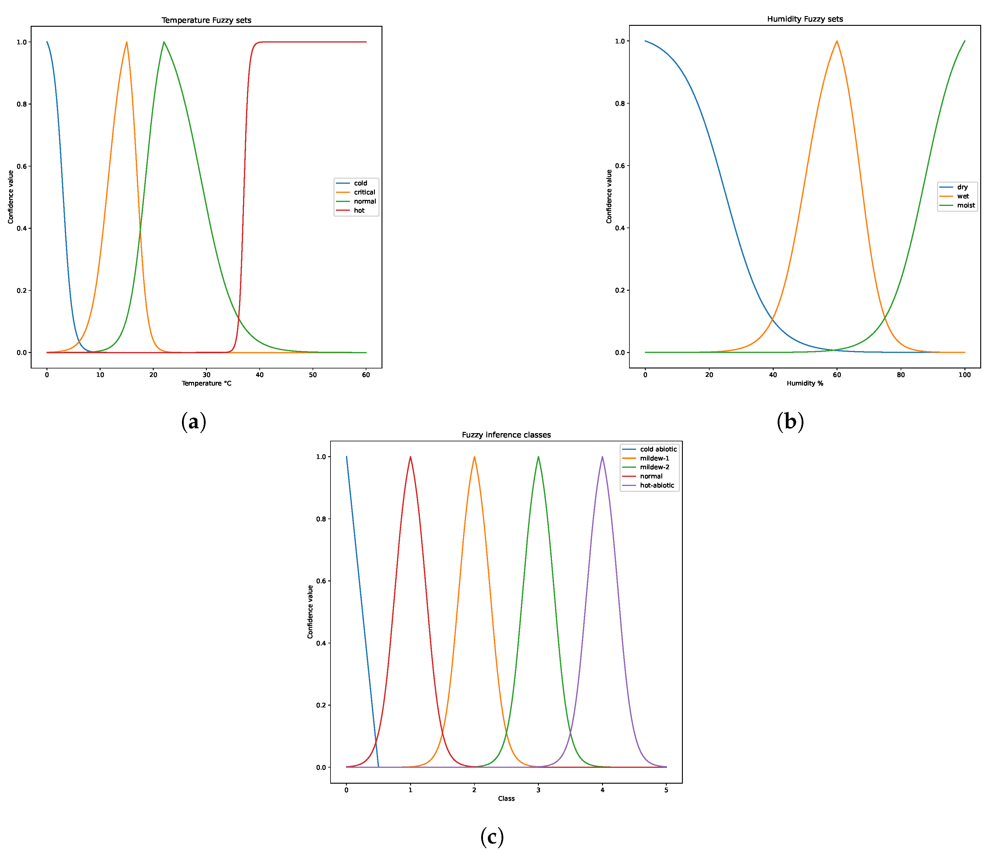
| Temperature (cold) | very (cold abiotic) | plus (cold abiotic) | cold abiotic |
| Temperature (critical) | very (mildew-1) | mildew-2 | very (mildew-2) |
| Temperature (normal) | very (normal) | minus (normal) | mildew-1 |
| Temperature (hot) | very (hot abiotic) | plus (hot abiotic) | minus (normal) |
| Hourly (2) | 30 min (4) | 15 min (8) | 10 min (12) | 1 min (120) | |
|---|---|---|---|---|---|
| Inference Period (h)-dT | Batch_Size | Batch_Size | Batch_Size | Batch_Size | Batch_Size |
| 6 h- | 12 | 24 | 48 | 72 | 720 |
| 8 h- | 16 | 32 | 64 | 96 | 960 |
| 12 h- | 24 | 48 | 96 | 144 | 1440 |
| 24 h- | 48 | 96 | 192 | 288 | 2880 |
| 48 h- | 96 | 192 | 384 | 576 | 5760 |
| Batch_Size | No. Hidden Layers | Per Layer Trainable Parameters |
|---|---|---|
| 16 | 2 | L16, L64 |
| 48 | 4 | L48, L32, L32, L16 |
| 64 | 4 | L64, L64, L32, L16 |
| 80 | 5 | L80, L64, L64, L32, L16 |
| 96 | 5 | L96, L64, L64, L32, L16 |
| 160 | 6 | L160, L128, L128, L64, L32, L16 |
| 480 | 7 | L480, L256, L256, L128, L64, L32, L16 |
| 960 | 8 | L960, L512, L512, L256, L128, L64, L32, L16 |
| Month_Year | Mean Rainfall (mm) | Mean VPD (kPa) |
|---|---|---|
| 05_2021 | 0.85 | 0.35 |
| 05_2022 | 0.83 | 0.57 |
| 05_2023 | 0.49 | 1.9 |
| 06_2021 | 1.37 | 0.27 |
| 06_2022 | 1.38 | 0.7 |
| 06_2023 | 0.76 | 0.87 |
| 07_2021 | 1.99 | 0.07 |
| 07_2022 | 2.01 | 0.2 |
| 07_2023 | 1.79 | 0.08 |
| 08_2021 | 1.97 | 0.13 |
| 08_2022 | 1.52 | 0.39 |
| 08_2023 | 1.41 | 0.5 |
Disclaimer/Publisher’s Note: The statements, opinions and data contained in all publications are solely those of the individual author(s) and contributor(s) and not of MDPI and/or the editor(s). MDPI and/or the editor(s) disclaim responsibility for any injury to people or property resulting from any ideas, methods, instructions or products referred to in the content. |
© 2024 by the authors. Licensee MDPI, Basel, Switzerland. This article is an open access article distributed under the terms and conditions of the Creative Commons Attribution (CC BY) license (https://creativecommons.org/licenses/by/4.0/).
Share and Cite
Kontogiannis, S.; Koundouras, S.; Pikridas, C. Proposed Fuzzy-Stranded-Neural Network Model That Utilizes IoT Plant-Level Sensory Monitoring and Distributed Services for the Early Detection of Downy Mildew in Viticulture. Computers 2024, 13, 63. https://doi.org/10.3390/computers13030063
Kontogiannis S, Koundouras S, Pikridas C. Proposed Fuzzy-Stranded-Neural Network Model That Utilizes IoT Plant-Level Sensory Monitoring and Distributed Services for the Early Detection of Downy Mildew in Viticulture. Computers. 2024; 13(3):63. https://doi.org/10.3390/computers13030063
Chicago/Turabian StyleKontogiannis, Sotirios, Stefanos Koundouras, and Christos Pikridas. 2024. "Proposed Fuzzy-Stranded-Neural Network Model That Utilizes IoT Plant-Level Sensory Monitoring and Distributed Services for the Early Detection of Downy Mildew in Viticulture" Computers 13, no. 3: 63. https://doi.org/10.3390/computers13030063