Article

Horizontal Learning Approach to Discover Association Rules

1
Department of Information Systems, Tel Aviv-Yaffo Academic College, Tel Aviv-Yafo 6818211, Israel
2
Department of Computer Science, Netanya Academic College, Netanya 4223587, Israel
*
Author to whom correspondence should be addressed.
Computers 2024, 13(3), 62; https://doi.org/10.3390/computers13030062
Submission received: 23 November 2023 / Revised: 23 January 2024 / Accepted: 22 February 2024 / Published: 28 February 2024

Abstract

:
Association rule learning is a machine learning approach aiming to find substantial relations among attributes within one or more datasets. We address the main problem of this technology, which is the excessive computation time and the memory requirements needed for the processing of discovering the association rules. Most of the literature pertaining to the association rules deals extensively with these issues as major obstacles, especially for very large databases. In this paper, we introduce a method that requires substantially lowers the run time and memory requirements in comparison to the methods presently in use (reduction from O ( 2 m ) to O 2 m 2 in the worst case).

1. Introduction

Association rules are “if-then” statements that indicate the probability of relationships between data items within large datasets in various types of databases. Association rules are or can potentially be utilized in a very wide range of domains, and in particular, they constitute a very powerful tool when applied to very large datasets. There have been a very large number of algorithms to conduct learning with the help of association rules. However, in the case of very large databases, numerous algorithms of associate rules learning run into severe difficulties due to computation time and memory requirement constraints. The most important contribution of the present paper is the introduction of an entirely new concept of learning, which substantially reduces computation time and memory requirements, thus allowing it to operate effectively (in comparison to the alternative methods), even when datasets are very large.
The importance of each technology is directly dependent on the scope of its actual and potential applications. The following examples, covering a wide variety of domains, demonstrate the importance of association rules:
  • Association rule learning can discover purchasing habits based on past purchases and browsing history and can assist in understanding customer behavior and preferences by identifying associations between customer attributes, interactions, and purchase history. This allows it to segment customers accordingly and tailor marketing campaigns and personalized recommendations to specific customer segments. Association rule learning can help identify relationships between different products or services that are frequently purchased together. This knowledge enables businesses to design effective cross-selling and up-selling strategies.
  • Association rules can be applied in text mining tasks, such as analyzing customer reviews, social media posts, or news articles. By identifying associations between words or topics, association rule learning can assist in sentiment analysis and content recommendation systems.
  • Association rules can assist physicians with medical diagnosis. Using relational association rule mining, we can identify the relationship between symptoms and illnesses.
  • Association rules can support sound public policy. Every government has census data. These data can be used to plan efficient public services (education, health, transport) as well as help public businesses (for setting up new factories, shopping malls, and even marketing products).
  • Association rules are integrated within an intelligent transportation system (ITS) to find the relation between all parameters of transportation. This enables a flexible, precise, on-time, and organized interconnected intelligent controlling transportation system.
  • Association rule mining can detect fraudulent activity, such as credit card usage, excessive insurance claims, misuse of communication access, and more.
  • Association rule mining is used to identify patterns in social media data that can inform the analysis of social networks. Discover interesting group behavior, profiling of social groups, etc., can trigger actions that will benefit the social media providers.
  • Association rules can analyze price fluctuations and identify relationships between product prices, promotions, and customer purchasing behavior. This information can assist in dynamic pricing strategies, competitor analysis, and optimizing pricing decisions.
  • Association rules can be utilized in risk analysis and decision support systems. By identifying associations between risk factors, events, or conditions, association rule learning helps with risk assessment to mitigate potential risks.
  • Association rule learning can optimize inventory management by identifying associations between product demand, seasonality, and purchasing patterns. This information aids in inventory forecasting, stock replenishment, and reducing inventory holding costs.
  • Association rules can be used in energy management systems to identify patterns and associations between energy consumption, environmental factors, and energy efficiency measures. This knowledge helps with optimizing energy usage, reducing waste, and implementing energy-saving strategies.
  • Association rules can be applied in quality control processes to identify relationships between product attributes, manufacturing parameters, and quality issues. This knowledge helps with detecting patterns that contribute to quality defects, improving manufacturing processes, and reducing defects.
This paper introduces a novel approach that discovers association rules by processing records (rows) in each dataset and not attributes (columns) as is reported in the literature. Our method addresses some of the most critical challenges when applying association rules to very large databases: memory limitation and excessive run time.

1.1. Basic Terms

The association rules process discovers associations among variables in a dataset. While it is a well-known research topic, in this subsection, we go through a quick overview of the basic concepts regarding association rules learning [1].
Let dataset T contain I = { i 1 , i 2 , , i n } records (rows) and D = { d 1 , d 2 , , d m } variables (columns, attributes). Also, let every entry in T contain a real value R . That is
T i l , d k R   F o r   a l l   1 i n , 1 k m
Additionally, we define the itemset X as a collection of variables from D such that
0 < X < | D |
Based on (2), we can define a k itemset as a set containing k items (attributes) that have the same value. Thus, we can define the support of each attribute d k as follows:
S u p p d k = i = 1 n T i l , d k ; T i l , d k R
to obtain a nominal value, or
S u p p N d k = i = 1 n T i l , d k | T | ; T i l , d k R
to compute the relative support of d k with respect to n, the size of the dataset T . In simple terms, the support metric counts the number of times variable d k = α appears in dataset T .
Now, let X and Y be two itemsets such that X Y = . That means that we do not allow variables to belong to two different itemsets. In other words, we do not allow itemsets to have a common attribute. We denote an association rule as X = > Y . From the probabilistic point of view, we can say “given X , what is the probability of Y ”. This probability (or confidence) can be defined as a function of the support as follows:
C o n f X = > Y = S u p p ( X Y ) S u p p ( X )
The relationships between itemsets define the association rules, and the confidence ( C o n f ) of the relation computes the probability that such a rule exists.
In the rest of this paper, we further elaborate on the problem, discuss proposed solutions, and finally present our approach to discovering association rules. Specifically, the rest of Section 1 includes a quick discussion on the subject and the inherent difficulties related to association rule mining. Section 2 presents an overview of the related work. In Section 3, we present and elaborate on the horizontal learning (HL) approach. Section 4 offers a concrete example using the HL algorithm. In Section 5, we further discuss and present measurements related to the performance of our algorithm.

1.2. General Discussion of the Association Rules Table (ART)

We propose a different approach for extracting association rules. While the classical approach has the complexity of O ( 2 m ) (where m is the number of attributes in the dataset), our approach yields O 2 m 2 in the worst case. The discovery process analyzes each record in the dataset, extracts possible itemsets, and computes their support.
The Association Rules Table (ART) is a 2-dimensional table containing an itemset and its count. The itemset can be the binary representation of any k itemset, and the counter is its support.
To simplify the process of discovering association rules from the ART, we convert dataset T into a binary representation (if it is not originally in the binary form). Figure 1 shows the overall process of creation of the ART.
The discovery process is quite straightforward: we process each line of the binary representation B separately. When the process of that line is completed, we process the next line (Figure 2).
Processing the line is the series of computations that we perform on a line.
When the processing of one line is completed, we move to the next record and repeat the process above. When the processing of the entire dataset is complete, all possible subsets are discovered (excluding the 0 subset) and placed on an A R T that contains all possible subsets and a counter that counts the number of occurrences of that subset throughout the entire dataset.
By the end of the process, the A R T will contain all possible subsets from the datasets (itemsets) and their counters (support). Analyzing the results, we demonstrate that while the run time of the classical approach is O ( 2 m ) (where m is the number of attributes in the dataset), our approach yields O ( 2 m / 2 ) in the worst case (Algorithm 1).
Algorithm 1: Creation of the ART.
For each record in the database do:
  • Count the number of non-empty entries in a record. This becomes the n-itemset.
  • While   n > 0 do:
  a.
Add   the   n -itemset to ART (see Section 3) and increment its count.
  
  b.
Compute all possible (n-1)-itemsets (subsets) of the n-itemset.
  c.
Add each (n-1)-itemsets to ART and increment their count.
  d.
n n 1
We will describe the algorithm, provide examples, and discuss the mathematical behavior of the algorithm in the sections below.

2. Related Work

2.1. Literature Survey

Association rules, first introduced in 1993 [1], are used to identify relationships among items in a database. These relationships are not based on inherent properties of the data themselves (as with functional dependencies) but rather based on the co-occurrence of the data items. The AIS algorithm was the first published algorithm developed to locate all large itemsets in a transaction database [1]. The method generates a very large number of candidate sets and for the truly Big Data cases, it can cause the memory buffer to overflow. Therefore, a buffer management scheme is necessary to handle this problem for large databases.
The simplest and most commonly used method to reduce the number of rules is applying a threshold to the support metric. This threshold (denoted m i n s u p p ) prevents variables with a small number of occurrences from being considered as part of any itemset and, therefore, part of any association rule. Thus, if the support of any itemset is less than the minimum support ( m i n s u p p ), we remove that itemset from any considerations of being part of some association rule [1]. This way we eliminate rules and thus reduce the computation complexity of Equations (6) and (7) (Section 2.2). On the other hand, the decision regarding the value of the minimum support remains questionable because eliminating itemsets of small support prevents us from discovering infrequent rules with high confidence.
Since the 1990s, a large number of algorithms have been developed and published. The following is a brief review of the literature most relevant to our method. The various algorithms presented below aim to improve accuracy and decrease the complexity and hence the execution time. However, there is usually a trade-off among these parameters.
The apriori algorithm [2] is the most well-known association rule algorithm. This technique uses the property that any subset of a large itemset must be a large itemset. Also, it assumes that items within an itemset are kept in lexicographic order. The AIS algorithm generates too many candidate itemsets that turn out to be small. On the other hand, the apriori algorithm generates the candidate itemsets by joining the large itemsets and deleting small subsets of the previous pass. By only considering large itemsets of the previous pass, the number of candidate itemsets is substantially reduced. The authors also introduced two modified algorithms: Apriori TID and Apriori Hybrid. The Apriori TID algorithm [2] is based on the argument that scanning the entire database may not be needed in all passes. The main difference from apriori is that it does not use the database for counting support after the first pass. Rather, it uses an encoding of the candidate itemsets used in the previous pass. The apriori approach performs better in earlier passes, and Apriori TID outperforms apriori in later passes. Based on the experimental observations, the Apriori Hybrid technique was developed. It uses apriori in the initial passes and switches later as needed to Apriori TID. The performance of this technique was also evaluated by conducting experiments for large datasets. It was observed that Apriori Hybrid performs better than apriori, except in the case when the switching occurs at the very end of the passes [3].
The Direct Hashing and Pruning (DHP) algorithm was introduced by Park et al. [4] to decrease the number of candidates in the early passes. DHP utilizes a hashing technique that attempts to restrict the number of candidate itemsets and efficiently generates large itemsets. These steps are designed to reduce the size of the database [4]. An additional hash-based approach for mining frequent itemsets was introduced by Wang and Chen in 2009. It utilizes a hash table to summarize the data information and predicts the number of non-frequent itemsets [5].
The Partitioning Algorithm [6] attempts to find the frequent elements by partitioning the database. In this way, the memory issues of large databases are addressed because the database is divided into several components. This algorithm decreases database scans to generate frequent itemsets. However, the time for computing the frequency of the candidate generated in each partition increases. Nevertheless, it significantly reduces the I/O and CPU overheads (for most cases).
An additional method is the Sampling Algorithm [7], where sample itemsets are taken from the database instead of utilizing the whole database. This algorithm reduces the database activity because it requires only a subsample of the database to be scanned [7]. However, the disadvantage of this method is less accurate results. The Dynamic Itemset Counting (DIC) [8] algorithm partitions the database into intervals of a fixed size. This algorithm aims to find large itemsets and uses fewer passes over the data in comparison to other traditional algorithms. In addition, the DIC algorithm presents a new method of generating association rules. These rules are standardized based on both the antecedent and the consequent [8].
There are additional methods based on horizontal partition, such as works by Kantarcıoglu and Clifton [9], Vasoya and Koli [10], and Das et al. [11]. These works attempt to partition the dataset, process each part separately, and then combine the results without the loss of small (with small minsupp) itemsets. Here, we have to emphasize that the horizontal partition utilized in the above-mentioned articles is not the same thing as the horizontal learning presented in our paper and is not as effective in addressing the complexity/memory requirements issues in comparison to our method.
The Continuous Association Rule Mining Algorithm (CARMA) [12] is designed to compute large itemsets online. The CARMA [12] shows the current association rules to the user and allows the user to change the parameters, minimum support, and minimum confidence at any transaction during the first scan of the database. It needs at most two database scans. Similar to DIC, the CARMA generates the itemsets in the first scan and finishes counting all the itemsets in the second scan. The CARMA outperforms apriori and DIC on low-support thresholds.
The frequent pattern mining algorithm (which is based on the apriori concept) was extended and applied to the sequential pattern analysis [13], resulting in the candidate generation-and-test approach, thus leading to the development of the following two major methods:
  • The Generalized Sequential Patterns Algorithm (GSP) [14], a horizontal data format-based sequential pattern mining algorithm. It involves time constraints, a sliding time window, and user-defined parameters [14];
  • The Sequential Pattern Discovery Using Equivalent Classes Algorithm (SPADE) [15], an Apriori-Based Vertical Data Format algorithm. This algorithm divides the original problem into sub-problems of substantially smaller size and complexity that are small enough to be handled in main memory while utilizing effective lattice search techniques and simple join operations [15].
Additional techniques that should be mentioned are based on the pattern–Growth-based approaches, and they provide efficient mining of sequential patterns in large sequence databases without candidate generation. Two main pattern–growth algorithms are frequent pattern-projected sequential pattern mining (FREESPAN) [13] and prefix-projected sequential pattern mining (PrefixSpan) [16]. The FREESPAN algorithm was introduced by Han et al. [17] with the objective of reducing workload during candidate subsequence generation. This algorithm utilizes frequent items and recursively transforms sequence databases into a set of smaller databases. The authors demonstrated that FREESPAN runs more efficiently and faster than an apriori-based GSP algorithm [13]. The PrefixSpan algorithm [16] is a pattern–growth approach to sequential pattern mining, and it is based on a divide-and-conquer method. This algorithm divides recursively a sequence database into a set of smaller projected databases and reduces the number of projected databases using a pseudo projection technique [16]. PrefixSpan performs better in comparison to GSP, FREESPAN, and SPADE and consumes less memory space than GSP and SPADE [16].
Another approach is the FP growth [17], which compresses a large database into a compact frequent pattern tree (FP tree) structure. The FP growth method has been devised for mining the complete set of frequent itemsets without candidate generation. The algorithm utilizes a directed graph to identify possible rule candidates within a dataset. It is very efficient and fast. The FP growth method is an efficient tool to mine long- and short-frequency patterns. An extension of the FP growth algorithm was proposed in [18,19] utilizing array-type data structures to reduce the traversal time. Additionally, Deng proposed in [20] the PPV, PrePost, and FIN algorithms, facilitating new data structures called node list and node set. They are based on an FP tree, with each node encoding with pre-order traversal and post-order traversal.
The Eclat algorithm introduced in [21] looks at each variable (attribute, item) and stores the row number that has the value of 1 (list of transactions). Then, it intersects the columns to obtain a new column containing the common IDs, and so on. This process continues until the intersection yields an empty result. For example, let the original matrix be as follows (Table 1).
Now, as a next step, if we intersect columns 1 and 2 , we obtain set { 5 } , and so on. Each time, the result is added to the matrix (see Table 2).
In [22,23,24], Manjit improved the Eclat algorithm by reducing escape time and the number of iterations via a top-down approach and by transposing the original dataset.
Refs. [6,11,25] describe algorithms that partition the database, find frequent itemsets in each partition, and combine the itemsets in each partition to obtain the global candidate itemsets, as well as the global support for the items. The approaches described above reduce the computation time and memory requirements and make the process of searching for candidates simple and efficient. However, they all compare columns in their quest to find the proper itemsets.
Prithiviraj and Porkodi [26] wrote a very comprehensive article in which they compare some of the most popular algorithms in the field. They concluded their research by creating a table that compares the algorithms by some criteria. This table (Table 3) is presented below.
Győrödi and Gyorodi [27] also studied some association rules algorithms. They compared several algorithms and concluded that the dynamic one (DynFP growth) is the best. Hence, in order to evaluate the performance of our horizontal learning algorithm, we compared the performance of horizontal learning to DynFP growth. The comparison is presented in Table 4.
The comparison above clearly demonstrates that horizonal learning performs better than other algorithms that were studied.

2.2. The Horizontal Learning Approach

When comparing columns, we need to count all 1 itemsets, 2 itemsets, and m itemsets. In addition, the dataset must be scanned once (each scan requires n comparisons) in order to compute the support. Let C t r a d be the traditional approach to computing the itemsets. Then, the total number of operations required for computing the itemsets is as follows:
C t r a d = n m 1 + n m 2 + + m m = n m ! 1 · m 1 ! + m ! 2 ! · m 2 ! + + m ! m ! · 1 ! = n ( 2 m 1 )
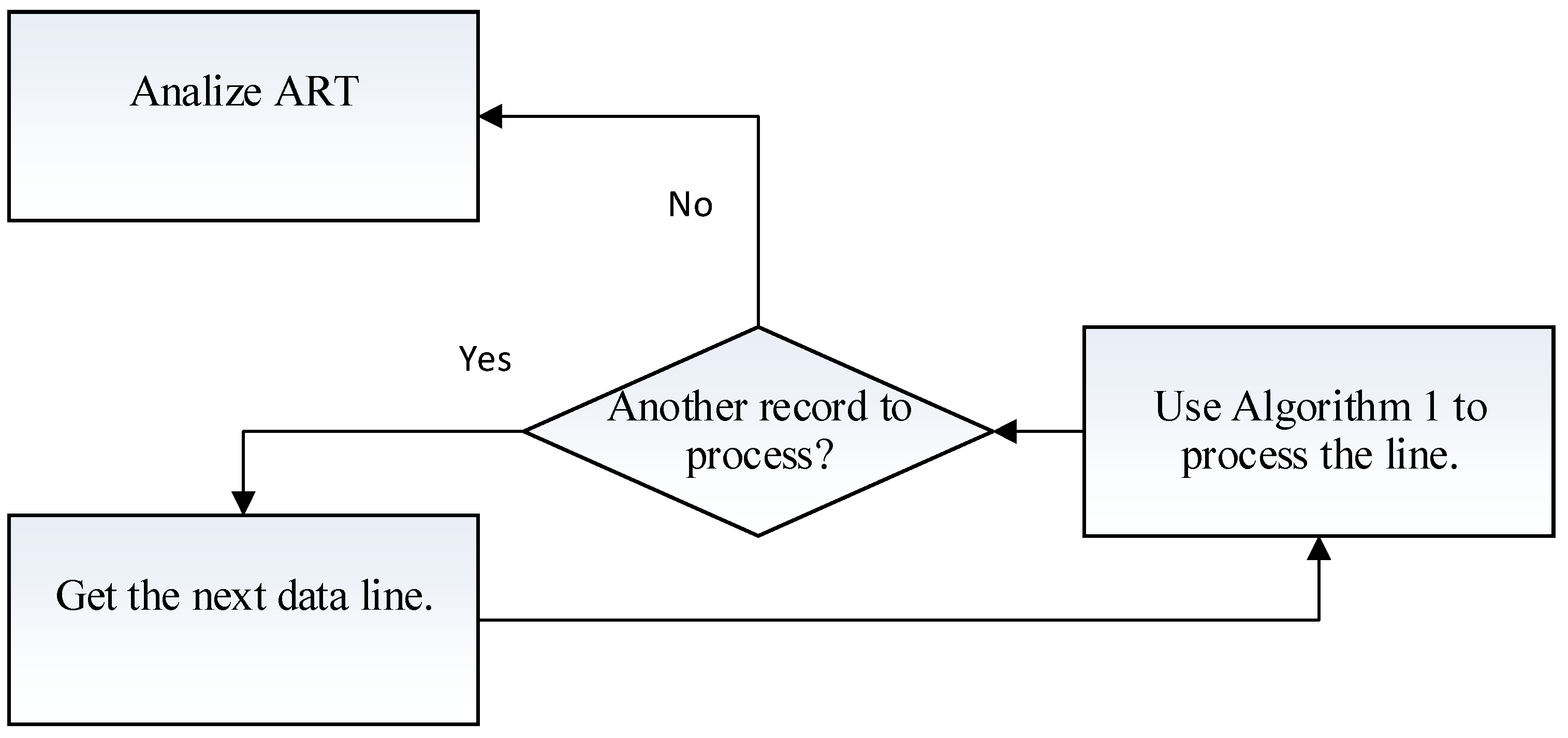
The horizontal learning approach (HL) is quite different. We analyze each record (row) in the dataset by extracting all the possible non-zero (non-blank for non-numerical data) values in that record. The possible values are stored in temporary set A . Then, we compute all possible subsets of A , excluding the 0 subset. For example, let a record contain the following data 00703 . Here, we have t w o non-zero values, so the possible subsets that can be generated will be 00700 , 00003 , and 00703 . These subsets will be stored in the special matrix C , and the counters for each string will be set to 1 . Later, we will present the formal algorithm for generating the subsets, but for simplicity, we will use a binary dataset.
Making an exaggerated (and very conservative) assumption that on average, half of the values in each row have a non-zero value and the number of variables in the dataset is m , this would yield 2 m 2 comparisons. Since there are n rows in the original database T , the execution time will be n · 2 m 2 . So, if we denote C H L as the itemset count (based on the horizontal learning approach), then
C H L = n · 2 m / 2
To compute the complexity of the algorithm, we define the number of variables (items) as m and the number of records as n . To be as conservative as possible, we assume that on average, the number of non-zero values in each record is m 2 . Under this assumption, the complexity of the process is as follows:
C m p l e x H L = O n · 2 m / 2
and the memory requirement of the process is as follows:
M = O 2 m
where C m p l e x H L is the processing complexity and M is the memory requirement. For example, for n = 1000 and m = 20 , then C = O 10 6 1   M c y c l e s and M = O ( 1   M b y t e ) .
When comparing Equations (6) and (7), we can erase coefficient n .
Figure 3 compares the two equations for m = [ 1 , 2 , 3 , , 20 ] , where m is the number of variables. The X-axis represents the number of variables, while the Y-axis represents the number of operations needed to generate association rules (computational complexity).

3. Horizontal Learning

The trade-off between the value of the minimum support and the information gained or lost is a bit troubling. Increasing the minimum support reduces the memory needed to store all phases of the process of discovering association rules. Therefore, the computation time becomes more manageable. On the other hand, removing some of the variables due to low support may cause a loss of potentially important information.
The task of the following algorithm is to obtain the association rules without forcing the activation of the minimum support.
Horizontal learning is a two-step process:
  • Convert the data matrix T into a better-represented binary matrix B;
  • Use matrix B to create the Association Rules Table (ART).

3.1. From Dataset T to a Binary Representation B

Let T be the matrix containing the original data. Also, let T contain m variables and n transactions. Also, let us assume that the data contained in T can be of any value and any type. The process of creating matrix B can be divided into three parts:
  • Create the header for the binary table B;
  • Optimize the header;
  • Add the appropriate data from the original dataset T.

3.1.1. Creating the Header for B

In this initial step, we scan the original database and create a two-dimensional vector. Since the original database T contains n records and m variables, the original dimensions of matrix B will be n m × 2 . For example, assume we have the following database (Table 5).
In this case, the header of B will contain one row of size eight (two variables multiplied by four rows) for the variable names and the second row for their value. This is shown in Table 6.
This is not optimal since there are columns that have the same values, and we want to create a header that contains only unique values. In Table 6, we can see that A1 = 5 is repeated twice. Also, A2 = 3 is repeated twice. We need to omit these columns.

3.1.2. Optimizing the Header for Binary Table B

After the header of matrix B is created, scan the header for repeated patterns. If found, they are omitted. The resulting header now contains only unique patterns. This is shown in Table 7.
Now, we can proceed to complete the binary table B by adding the locations of each of the values created in the header of matrix B.

3.1.3. Completing the Construction of B

The algorithm for completing the construction of matrix B is as follows (Algorithm 2).
Algorithm 2: The process of completing matrix B.
For   i = 1   to   n   do   ( n is the amount of rows in T)
For   j = 1   to   m   do   ( m is the amount of columns in T)
  •  Get   the   value   in   T i , j
  • Find its location (j) in the header of matrix B
When the process is completed, matrix B (Table 8) will contain all the needed information for finding the association rules.
We can apply the same process when database T contains alpha-numeric data. Assume we have the following database.
A1A2
1Tom4
2Tim3
3Jin1
4Tim3
We apply the conversion process as described above. This will yield the following binary representation.
A1A1A1A2A2A2
TomTimJin431
1100100
2010010
3001001
4010010
Now that we have a binary matrix, we can use the horizontal learning process to generate the Association Rules Table. In other words, since we have generated a binary table, we can use any of the algorithms described in the literature survey to find association rules.
However, due to the issues of complexity and memory limits mentioned above (in the case of very large datasets), we introduce a different representation (the ART representation) that will speed up the process and enable the user to choose his/her preferences by controlling various parameters.

3.2. From Matrix B to the ART

The purpose of the following algorithm (Algorithm 3) is to create an environment in which all the necessary information regarding the construction of the association rules will be available and that the process will be conducted fast.
Algorithm 3: The process of completing matrix B .
For   i = 3   to   n + 2 do (n is the amount of data rows in B)
  a.
Get the ith record. This record represents some k-itemset.
  b.
Find all possible j-itemsets, such that 0 < j k
  c.
If the j-itemset is found in ART, add 1 to counter. Else add the j-itemset to the ART and set its counter to 1.
An important issue to discuss here is the reason for finding all sub-itemsets for a given k itemset. Recall Equations (3)–(5). In order to compute the confidence of a rule generated from some k itemset, it is essential to know the support of the sub-itemsets. By computing all possible support of all possible sub-itemsets, we guarantee that the ART contains all the necessary information to generate the association rules.
When the process of creating the ART is completed, each row in the A R T represents an itemset and a counter, which is the support. For example, the first line in B is {1 0 0 1 0 0}. The possible itemsets are as follows:
{1 0 0 0 0 0}
{0 0 0 1 0 0}
{1 0 0 1 0 0}
These three itemsets are added to the ART and their counter is set to 1. This process continues until all records in B are processed. A more comprehensive example will be given next.

3.3. A Comprehensive Example of Moving from Matrix B to the ART

As was discussed above, the horizontal learning algorithm can handle both binary and non-binary data. In this section, we show how to create the matrix ART, where the dataset is binary (either originally or transformed as described in the previous section). Let our database T be as follows.
123456
11 1 1
2 1 1
3 11
41 1 1
511 11
6 1
71 11
8 1
91 1
101 11
1111 111
Generally, let p be the number of non-zero values in a row; then, the number of possible sub-itemsets that we can generate is 2 p 1 . The reason we subtract 1 from the total is because we exclude the possibility that no value is selected. Starting with row 1 , it contains 1 s in locations, 1 , 4 , and 6 . This means that we can generate seven different sub-records. They are shown below.
000001
000100
100000
000101
100001
100100
100101
One way to compute all possible combinations is breaking the k itemset into k 1 itemsets and building on that. In our example, k = 3, so we create three 1 itemsets.
000001
000100
100000
Based on the above information we can generate all possible 2 itemsets.
000101
100001
100100
And finally, we generate the 3 itemset.
100101
After this information is calculated, we can add it to the ART.
ItemsetCount
0000011
0001001
0001011
1000001
1000011
1001001
1001011
The second row in the example contains 1 s in columns 2 and 5 . We repeat the process to obtain the following information.
000010
010000
010010
We add this information to the ART.
ItemsetCount
0000011
0000101
0001001
0001011
0100001
0100101
1000001
1000011
1001001
1001011
We continue the process until we scan the entire original database T . Since each entry in the A R T represents a possible itemset and since the count is the support ( S u p p ) of any subset, we can summarize the results of the process in Table 9.

3.4. Moving Directly from T to the ART

We can construct the matrix ART directly from the original database T . It is more effective and much faster but lacks the ability to have a nice display.
For example, the first record in Table 10 contains values {1, 4}. From that record, we can generate all possible sub-records, {0, 1}, {4, 0}, and {1, 4}, and set their counters to 1. This procedure is very fast and is a space saver, but it is harder to read than a binary sequence. It is up to the users to decide their preferences.
In any case, the complete transformation of T to the ART using Algorithm 4 is depicted in Table 10.
Algorithm 4:  Constructing   the   ART   table   directly   from   database   T .
For   i = 1   to   n do (n is the number of data rows in T)
  a.
Get the ith record. This record represents some k-itemset.
  b.
Find all possible j-itemsets, such that 0 < j k .
  c.
If the j-itemset is found in ART, add 1 to counter. Else add the j-itemset to the ART and set its counter to 1.

4. Discussion

Table 11 provides all the necessary information we need to construct the possible association rules. First, we can see that 27 out of 64 (almost 50%) possible itemsets are not participating in the construction of the itemsets since their support is zero. In our practical applications of the method, the percentage has consistently been much smaller. One small example will illustrate this point. When a customer enters a store to buy some products, it is not reasonable to expect that he/she will buy up to 50% of the products sold in that store. It is more reasonable to expect that only a very small percentage of the products will be purchased. This is also the reason for the assumption in Equation (8) in Section 2.2, which, as we stated above, is very conservative. Therefore, if we design the A R T as a hash matrix, we will utilize only half of the memory to store the relevant itemsets.
Now, assume we want to generate all the rules associated with the string   100110 . We have six choices.
c o n f 100000 000110 = S u p p 100110 S u p p 100000 = 3 7 c o n f 000100 100010 = S u p p 100110 S u p p 000100 = 3 7 c o n f 000010 100100 = S u p p 100110 S u p p 000010 = 3 4 c o n f 100100 000010 S u p p 100110 S u p p 100100 = 3 6 c o n f 100010 000100 = S u p p 100110 S u p p 100010 = 3 3 c o n f 000110 100000 = S u p p 100110 S u p p 000110 = 3 6
If we set the minimum confidence to 0.8 , then only one rule is chosen.
c o n f 100010 000100 = S u p p 100110 S u p p 100010 = 1
Let v i be the i th attribute. Then, the rule above can be translated to
i f v 1 = 1   a n d   v 4 = 1   t h e n   ( v 3 = 1 )
This means that every time attributes 1 and 5 are set to 1 , so is attribute 4 . We can confirm the result by observing Table 11.
In many applications, we want to find infrequent rules, such as rules that can be derived from the string 100001 . In this case, we can generate t w o rules as follows:
c o n f 100000 000001 = S u p p 100001 S u p p 100000 = 3 7 c o n f 000001 100000 = S u p p 100001 S u p p 000001 = 3 3 .
From the above, we can see that each time v 6 is set to 1 , so is v 1 .
We can also define the minimum support (say m i n s u p p = 3 ), an action that will result in a reduction in the A R T , as shown in Table 11.
We can also search for the largest/smallest itemset given some minimum support. For example, based on Table 11, we see that the largest itemset is in the string 100110 . In this case, we can generate s i x possible rules. We can also see that there are f o u r itemsets with t w o   1 s in them. So, we can generate an additional e i g h t different rules. In total, we can generate 14 possible rules from the original database (without considering the confidence factor).

5. Evaluation

The ART generates the association rules based on the specified support and the confidence of the rule. Now, we need to test the idea in practice. We compare the set of rules generated by the learning algorithm with each record in the testing to find out if the association rules are working successfully.
To evaluate an association rule, we need to define a procedure by which we can measure the effectiveness/correctness of the rule. To do so, we define the coverage of the rule.
Recall that an association rule has the general format of X Y , where both X and Y are itemsets. The coverage of a rule means how well the association rule is covering a line (record) in a dataset. In other words, if we check that all the items in X are found in given records, that means that the premise coverage of that record is full. If not, then the coverage is 0. (It is possible to use partial coverage, but this is not within the scope of this paper). If the premise coverage of the rule is 1 (full coverage), we can compute the coverage of the conclusion of the association rule ( Y ). Again, if all the items in Y are part of the record in question, the conclusion coverage is full, and we set the evaluation grade to 1; otherwise, the grade is set to zero. Here, we can also use a partial match.
In order to further investigate our approach, we have chosen t h r e e datasets (denoted as D S 1 , D S 2 , and D S 3 ). All t h r e e datasets contain f o r t y t h r e e attributes (variables). D S 1 contains 4000 records, D S 2 contains 7000 records, and D S 3 contains 8000 records.
We implemented the HL algorithm and learned new association rules using D S 1 . In order to understand more about the influence of the support on the quality of the rules, we divided the support into small groups (Supp = [3..15]) all the way to Supp = [200..1000]. The following table shows the number of rules generated by the HL affected by the value of the support.
Support3–1510–5025–10050–200150–400200–1000
Rules2216291311430
As can be seen, when the size of the support is small (up to 15 occurrences in the dataset), the number of rules generated is 22. As we increased the support, the number of rules increased.
Next, we tested it against DS2 and DS3. The results are displayed in Table 12.
The first row in Table 12 shows the support used to test the algorithm. For example, values 10–50 indicate that we are looking for itemsets having support between 10 and 50 . The second row displays the number of rules generated using the support defined earlier.
The “Total” rows indicate the number of cases in which the matching of the premise of a rule and any given data line was above the matching threshold (in the above table, it was set to 100%). The “Success” lines show the number of times the premise was matched and the conclusion. In other words, if the premise of some rule is matched against some data line, so was the conclusion, and we mark it as a success. If the premise of some rules is matched against a data line but the conclusion does not match, we mark it a “Fail”.
An additional example can be seen in the last column in Table 11 . We used the support of 200 to 1000 to generate 30 different rules. When we tested it with D S 3 , we found out that the system found 14,678 cases in which the rules were matched against the data lines in D S 3 . From these, in 12,080 cases, we also found a match in the conclusion. This indicates that we were successful in the rule generation. In 2598 cases, we were successful in matching the data line against the premise of the rules but failed to match the data line against the conclusions of the association rules.

6. Conclusions

In this paper, we presented a new algorithm that is capable of mining association rules from datasets. Its main contribution is the capability of our method to substantially reduce the process complexity, reflected in a greatly diminished run time and memory requirements, which are two main obstacles for associate rules mining in very large databases.
Specifically, we demonstrated how to generate the possible itemsets that constitute different association rules. For that, we created the Association Rules Table (ART) containing all possible and necessary information needed to generate the association rules.
From this table, we can generate all possible types of association rules. We can generate infrequent as well as frequent association rules. We can create rules from any combination we choose by clicking the specific entries in the ART.
In order to validate our method, we utilized large datasets containing 43 attributes (variables) and 19,000 records. The results of the testing (see Table 11) clearly indicate a very high success rate.

Author Contributions

Conceptualization, E.S.; Methodology, A.Y. and A.B.; Software, M.S.; Formal analysis, I.R.; Investigation, A.B. and I.R.; Data curation, A.B. All authors have read and agreed to the published version of the manuscript.

Funding

This research received no external funding.

Data Availability Statement

Data are contained within the article.

Conflicts of Interest

The authors declare no conflict of interest.

References

  1. Agrawal, R.; Imieliński, T.; Swami, A. Mining association rules between sets of items in large databases. In Proceedings of the 1993 ACM SIGMOD International Conference on Management of Data—SIGMOD’93, Washington, DC, USA, 26–28 May 1993; p. 207. [Google Scholar]
  2. Agrawal, R.; Srikant, R. Fast algorithms for mining association rules. In Proceedings of the Twentieth International Conference on Very Large Databases (VLDB), Santiago, Chile, 12–15 September 1994; pp. 487–499. [Google Scholar]
  3. Srikant, R. Fast Algorithms for Mining Association Rules and Sequential Patterns. Ph.D. Dissertation, University of Wisconsin, Madison, WI, USA, 1996. [Google Scholar]
  4. Park, J.S.; Chen, M.S.; Yu, P.S. An Effective Hash-based Algorithm for Mining Association Rules. In Proceedings of the 1995 ACM SIGMOD International Conference on Management of Data—SIGMOD’95, San Jose, CA, USA, 22–25 May 1995; pp. 175–186. [Google Scholar]
  5. Wang, E.T.; Chen, A.L. A Novel Hash-based Approach for Mining Frequent Itemsets over Data Streams Requiring Less Memory Space. Data Min. Knowl. Discov. 2009, 19, 132–172. [Google Scholar] [CrossRef]
  6. Savasere, A.; Omiecinski, E.; Navathe, S. An efficient algorithm for mining association rules for large databases. In Proceedings of the 21th International Conference on Very Large Data Bases, Zurich, Switzerland, 11–15 September 1995; pp. 432–444. [Google Scholar]
  7. Toivonen, H. Sampling Large Databases for Association Rules. In Proceedings of the 22th International Conference on Very Large Databases (VLDB’96), Bombay, India, 3–6 September 1996; pp. 134–145. [Google Scholar]
  8. Brin, S.; Motwani, R.; Ullman, J.D.; Tsur, S. Dynamic Itemset Counting and Implication Rules for Market Basket Data. In Proceedings of the 1997 ACM SIGMOD International Conference on Management of Data, Tucson, AZ, USA, 13–15 May 1997; Volume 26, pp. 255–264. [Google Scholar]
  9. Kantarcioglu, M.; Clifton, C. Privacy-preserving Distributed Mining of Association Rules on Horizontally Partitioned Data. IEEE Trans. Knowl. Data Eng. 2004, 16, 1026–1037. [Google Scholar] [CrossRef]
  10. Vasoya, A.; Koli, N. The Parallelization of Algorithm based on Horizontal Partition for Association Rule Mining on Large Data Set. Int. J. Eng. Res. Technol. (IJERT) 2020, 6, 85. [Google Scholar]
  11. Das, A.; Bhattacharyya, D.K.; Kalita, J.K. Horizontal vs. Vertical Partitioning in Association Rule Mining: A Comparison. In Proceedings of the 6th International Conference on Computational Intelligence and Natural Computation (CINC), Cary, NC, USA, 26–30 September 2003. [Google Scholar]
  12. Hidber, C. Online association rule mining. In Proceedings of the 1999 ACM SIGMOD International Conference on Management of Data, Philadelphia, PA, USA, 1–3 June 1999; Volume 28, pp. 145–156. [Google Scholar]
  13. Han, J.; Pei, J.; Mortazavi-Asl, B.; Chen, Q.; Dayal, U.; Hsu, M.C. FREESPAN: Frequent Pattern-projected Sequential Pattern Mining. In Proceedings of the 2000 ACM SIGKDD International Conference Knowledge Discovery in Databases (KDD’00), Boston, MA, USA, 20–23 August 2000; pp. 355–359. [Google Scholar]
  14. Srikant, R.; Agrawal, R. Mining Sequential Patterns: Generalizations and Performance İmprovements. In Proceedings of the 5th International Conference Extending Database Technology (EDBT’96), Avignon, France, 25–29 March 1996; pp. 3–17. [Google Scholar]
  15. Zaki, J.M. SPADE: An efficient algorithm for mining frequent sequences. Mach. Learn. 2001, 42, 31–60. [Google Scholar] [CrossRef]
  16. Pei, J.; Han, J.; Asl, J.M.; Pinto, H.; Chen, Q.; Dayal, U.; Hsu, M.C. Prefix Span: Mining Sequential Patterns Efficiently by Prefix-Projected Pattern Growth. In Proceedings of the 17th International Conference on Data Engineering (ICDE), Heidelberg, Germany, 2–6 April 2001. [Google Scholar]
  17. Han, J.; Pei, J.; Yin, Y. Mining Frequent Patterns Without Candidate Generation. In Proceedings of the 2000 ACM SIGMOD International Conference on Management of Data—SIGMOD’00, Dallas, TX, USA, 16–18 May 2000; pp. 1–12. [Google Scholar]
  18. Grahne, O.; Zhu, J. Efficiently Using Prefix-trees in Mining Frequent Itemsets. In Proceedings of the IEEE ICDM Workshop on Frequent Itemset Mining, Brighton, UK, 1 November 2004. [Google Scholar]
  19. Grahne, G.; Zhu, J. Fast Algorithm for frequent Itemset Mining Using FP-Trees. IEEE Trans. Knowl. Data Eng. 2005, 17, 1347–1362. [Google Scholar] [CrossRef]
  20. Deng, Z.H.; Wang, Z. A New Fast Vertical Method for Mining Frequent Patterns. Int. J. Comput. Intell. Syst. 2010, 3, 733–744. [Google Scholar]
  21. Zaki, M.J. Scalable algorithms for association mining. IEEE Trans. Knowl. Data Eng. 2000, 12, 372–390. [Google Scholar] [CrossRef]
  22. Omiecinski, E.R. Alternative interest measures for mining associations in databases. IEEE Trans. Knowl. Data Eng. 2003, 15, 57–69. [Google Scholar] [CrossRef]
  23. Liu, J.; Paulsen, S.; Sun, X.; Wang, W.; Nobel, A.; Prins, J. Mining Approximate Frequent Itemsets in the Presence of Noise: Algorithm and Analysis. In Proceedings of the 2006 SIAM International Conference on Data Mining, Bethesda, MD, USA, 20–22 April 2006; pp. 407–418. [Google Scholar]
  24. Manjit, K. Advanced Eclat Algorithm for Frequent Itemsets Generation. Int. J. Appl. Eng. Res. 2015, 10, 23263–23279. [Google Scholar]
  25. Pujari, A.K. Data Mining Techniques; Universities Press (India) Ltd.: Hyderabad, India, 2001. [Google Scholar]
  26. Prithiviraj, P.; Porkodi, R. A Comparative Analysis of Association Rule Mining Algorithms in Data Mining: A Study. Am. J. Comput. Sci. Eng. Surv. AJCSES 2015, 3, 98–119. [Google Scholar]
  27. Győrödi, C.; Gyorodi, R. A Comparative Study of Association Rules Mining Algorithms. In Proceedings of the SACI 2004, 1st Romanian—Hungarian Joint Symposium on Applied Computational Intelligence, Timisoara, Romania, 25–26 May 2004. [Google Scholar]
Figure 1. General flowchart of the creation of the ART.
Computers 13 00062 g001
Figure 2. General flow of the horizonal learning process.
Computers 13 00062 g002
Figure 3. Comparing the HL algorithm to the apriori approach.
Computers 13 00062 g003
Table 1. Vertical (left) and horizontal display (right) of a sample dataset.
TID A B C D
1A D 1 2 3 1
2B 4 5 4 3
3C D 5 6 5
4A C 7 8 7
5A B D
6B
7A D
8B
Table 2. Adding two itemsets to Table 1.
ABCD A B
1 2315
4 543
5 6 5
7 8 7
Table 3. Comparison of some leading association rules algorithms.
AlgorithmAlgorithm Data SupportMeritsDemerits
Apriori (2003)Best used for closed itemsets.Fast.
Uses minsupp to eliminate small itemsets.
Takes a lot of memory.
Apriori TID (1994)Used for minor itemsets.Better than SETM.
Better than apriori for small databases.
Time saving.
Does not use the whole database to count candidate sets.
SETM (1994)Not frequently used.Separates generation from counting.Very large execution time.
The size of the candidate set is large.
Apriori Hybrid (1994)Used where apriori and Apriori TID are used.Better than both apriori and Apriori TID.An extra cost is incurred when shifting from apriori to Apriori TID
AIS (1994)Not frequently used, but when used, it is used for small itemsets.Better than SETM.Easy to use candidate sets generated on the fly.
The size of the candidate set is large.
FP Growth (2003)Used in cases of large itemsets, as it does not require the generation of candidate sets.Only two passes of the dataset.
Compresses the dataset.
No candidate set generation is required, so it is better than Eclat and apriori.
Using a tree structure creates complexity.
Table 4. Comparison of FP growth to horizontal learning.
FP Growth (2003)Used in cases of large itemsets, as it does not require the generation of candidate sets.Only two passes of the dataset.
Compresses the dataset.
No candidate set generation is required, so it is better than Eclat and apriori.
Using a tree structure creates complexity.
Horizontal Learning (2023)Used for any size dataset.Only one path through the dataset.Use a 2-dimentional hash table to represent all necessary information to generate association rules.
Table 5. Example of database T .
.A1A2
114
253
321
453
Table 6. Creating the header for B.
A1A1A1A1A2A2A2A2
15254313
Table 7. Optimized header for matrix B.
A1A1A1A2A2A2
152431
Table 8. The complete binary matrix B.
A1A1A1A2A2A2
152431
1100100
2010010
3001001
4010010
Table 9. The final state of the ART.
ISSupISSupISSupISSup
000000 010000510000071100002
0000013010001110000131100011
0000104010010310001031100102
0000111010011110001111100111
0001007010100210010061101002
0001012010101110010121101011
0001103010110210011031101102
0001111010111110011111101111
0010003011000 1010002111000
0010011011001 1010011111001
001010 011010 101010 111010
001011 011011 101011 111011
0011002011100 1011001111100
001101 011101 101101 111101
001110 011110 101110 111110
001111 011111 101111 111111
Table 10. Moving from T to the ART.
Database ART
A1A2Computers 13 00062 i001ItemsetSupportk-Itemset
1141 011
2530 411
3211 412
4535 021
5 0 321
6 5 322
7 2 011
8 0 111
9 2 112
As we will see later, in order to find association rules, we need to obey two rules. 1. The support of an itemset must be above a predefined minimum support. 2. The number of items in the itemset must be above 1.
Table 11. Reduction in the ART after applying minimum support.
ItemsetCountItemsetCount
00000130100103
00001041000007
00010071000013
00011031000103
00100031001006
01000051001103
Table 12. Simulation results.
Support3–1510–5025–10050–200150–400200–1000
Rules2216291311430
DS2_Total156969 4423356939,74414,661
DS2_Success988654354354738,07912,211
DS2_Failure58104692216652450
DS3_Total141945 4509356939,25614,678
DS3_Success788324437354737,97612,080
DS3_Failure63113 722212802598
Disclaimer/Publisher’s Note: The statements, opinions and data contained in all publications are solely those of the individual author(s) and contributor(s) and not of MDPI and/or the editor(s). MDPI and/or the editor(s) disclaim responsibility for any injury to people or property resulting from any ideas, methods, instructions or products referred to in the content.

